A Method Based on CNN–BiLSTM–Attention for Wind Farm Line Fault Distance Prediction

Abstract

In view of the complex operating environments of wind farms and the characteristics of multi-branch mixed collector lines, in order to improve the accuracy of single-phase grounding fault location, the convolutional neural network (CNN), bidirectional long short-term memory network (BiLSTM), and attention mechanism (attention) were combined to construct a single-phase grounding fault location strategy for the CNN–BiLSTM–attention hybrid model. Using a zero-sequence current as the fault information identification method, through the deep fusion of the CNN–BiLSTM–attention hybrid model, the single-phase grounding faults in the collector lines of the wind farm can be located. The simulation modeling was carried out using the MATLAB R2022b software, and the effectiveness of the hybrid model in the single-phase grounding fault location of multi-branch mixed collector lines was studied and verified. The research results show that, compared with the random forest algorithm, decision tree algorithm, CNN, and LSTM neural network, the proposed method significantly improved the location accuracy and is more suitable for the fault distance measurement requirements of collector lines in the complex environments of wind farms. The research conclusions provide technical support and a reference for the actual operation and maintenance of wind farms.

1. Introduction

Human beings have turned their attention to the field of new energy, including wind energy, solar energy, etc. The continuous global concern over energy issues has driven countries to implement strong support policies for new energy. In China, wind power technology has developed rapidly, and wind power energy has been increasingly incorporated into the power system. However, due to the unique operating mode of the collection lines in wind farms, besides issues such as randomness, volatility, and fault location, new challenges have been brought regarding the dynamic economic dispatching of the traditional power system. The speed and accuracy of fault location are crucial for the guidance of line inspection work and improvements in the line inspection efficiency, reducing the impact time of faults on grid connection. Progress in this research area can bring obvious economic and social benefits. The fault analysis method has high stability. However, the positioning accuracy is relatively sensitive to changes in the grounding resistance and line parameters. The inherent disparities in the physical and electrical properties between cables and overhead lines result in the reduced effectiveness of both conventional traveling-wave-based fault location techniques and standard fault analysis approaches when implemented on hybrid transmission line configurations. This analytical approach computes connection point electrical parameters using terminal voltage and current measurements, identifies the faulted branch through amplitude characteristic comparisons, and ultimately performs iterative calculations of the fault location based on the associated branch parameters. This method is only applicable to hybrid lines with a simple structure. For the collection lines of wind farms with many branches, the error will increase with the increase in branch points, thereby reducing the ranging accuracy. The traveling wave method exhibits low ranging complexity while maintaining immunity to variations in transition resistance and diverse fault conditions.

Regarding fault location in collector lines, current research achievements are relatively limited. Reference [1] describes an active excitation methodology employing FFT analysis to extract the zero-sequence current’s low-frequency components. These spectral characteristics undergo sequential threshold comparison for the precise identification of faulted segments in resonant grounded distribution systems. This scheme requires a step-by-step search for the faulty sections of the feeder. Meanwhile, it also has significant negative impacts, such as high redundancy and low positioning efficiency in the calculation process. Reference [2] adopts dual-voltage deviation indices (line and phase) as diagnostic criteria, extracts distinctive signatures per index through feature engineering, and ultimately employs pattern recognition to classify fault conditions.

The enhanced automation in wind farm operations has enabled the widespread deployment of intelligent terminal units and precision measurement instruments within AC/DC hybrid grids, establishing critical data foundations for deep learning implementations in complex wind farm fault localization. The regression mechanism of neural networks provides an idea for the fault location of collector lines by using neural networks. Reference [3] describes a diagnostic framework for multi-terminal direct current transmission systems, designing a dual-path convolutional neural network architecture that integrates separate classification and localization modules. Reference [4] develops a three-tier fault management framework for transmission networks in extended multi-machine grids, employing LSTM-based deep learning architectures to achieve integrated detection, diagnosis, and localization capabilities. After this method realizes fault diagnosis by using LSTM, it uses the LSTM regression mechanism to locate various faults in the faulty line. However, when facing three-phase grounding faults, its location error is relatively large. Building upon S-transform feature extraction in the literature [5], the optimized 1D-CNN–GRU architecture enables direct fault positioning in HVDC transmission infrastructures, eliminating prerequisite fault categorization. A comparative analysis reveals that zero-sequence current techniques exhibit superior efficacy for neutral isolated wind farm configurations when contrasted with conventional traveling-wave-based and fault-analytical approaches, where neural architectures subsequently enable predictive fault mapping. In reference [6], the CNN and LSTM are combined. Firstly, different transmission lines are divided according to the maximum average difference, and then the double-ended CNN–LSTM of Q-learning is combined to locate the faults of different types of transmission lines. Reference [7] directly takes the fault time series signal as the input and adopts the bidirectional gated recursive unit combined with an attention mechanism to achieve fault location, which is less affected by noise.

To address these challenges, this study introduces a CNN–BiLSTM–attention-driven localization framework specifically designed for wind farm collector line fault diagnosis. For a successful fault location management system, the analysis of collector line faults usually requires three main aspects: (1) a fault dataset; (2) adjustment of the parameters of the neural network models; (3) the implementation of the trained model for real-time fault localization in operational systems. For the extraction of fault features, we first model the wind farm through the MATLAB R2022b/SIMULINK software to extract the fault waveforms from the collector lines, and we then use the fast Fourier transform to extract other features, such as the voltage and current of the faults, as the fault set of the neural network. The next step is to input the data into the neural network that has been initially built and then continuously adjust the parameters of the model.

2. Fault Location Principle for Cable–Overhead Hybrid Transmission Lines

The power generated by wind turbine units is stepped up to 35 kV through step-up box transformers and then transmitted via cable segments to the overhead lines. The power from all wind turbine units converges on the collector lines and is routed through cables to the 35 kV low-voltage bus at the step-up substation. The wind farm is configured with ten wind turbine generators, each rated at 1.5 MW, with a rotational speed of 10 rpm. To simulate spatial wind speed variability across individual turbines—characteristic of operational wind farms—a random number block implements dynamic aerodynamic modeling [8,9,10,11].

The collector bus of the wind farm is connected to a zig-zag grounding transformer; therefore, the zero-sequence current generated during a ground fault flows through this path.

2.1. Fault Data Extraction

The zero-sequence current data in this study were processed using MATLAB for waveform spectral analysis. In time-domain waveform processing, the Fourier transform is typically employed to convert “time-domain functions” into “frequency-domain functions”, thereby transforming temporal variables into frequency variables. The Fourier transform was applied to extract features from both the fault-induced zero-sequence current waveforms and the three-phase current/voltage waveforms [12,13].

$$F\left(\omega \right)={\int }_{-\infty }^{\infty }f\left(t\right)e^{-j\omega t}dt$$

(1)

In Equation (1), $\mathrm{F}\left(\mathsf{\omega }\right)$ represents the frequency-domain function obtained via the Fourier transform, while $\mathrm{f}\left(\mathrm{t}\right)$ denotes the time-domain signal.

2.2. Fault Section Location

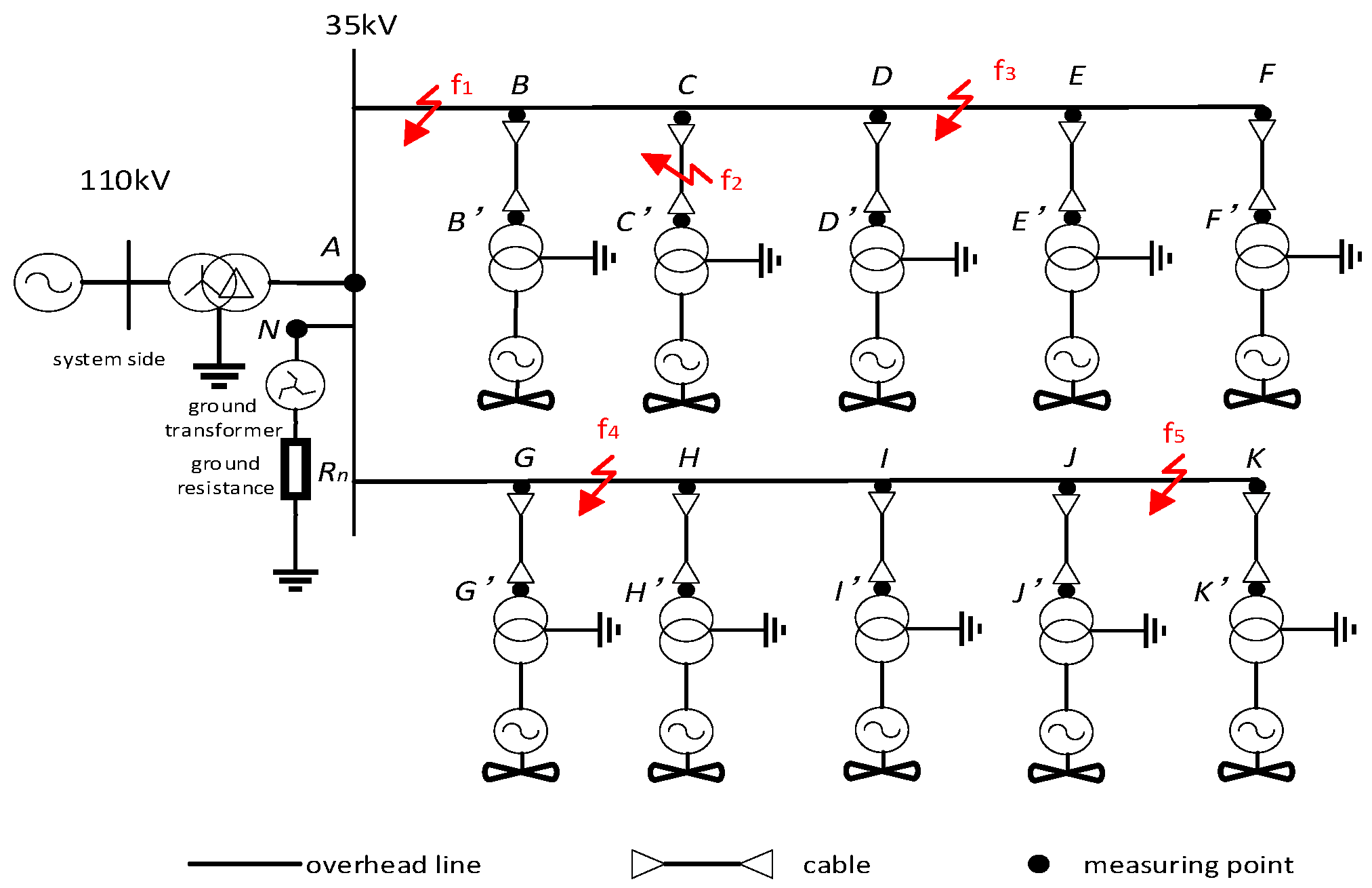
To demonstrate the fault zone identification criteria, the simplified wind farm model illustrated in Figure 1 is employed. Dual measurement nodes (A/B/C and A’/B’/C’) along the collector lines synchronously acquire three-phase electrical parameters and zero-sequence waveforms from respective branches [14,15,16,17].

(1)

An analysis of the wind farm configuration reveals that both the grid-connected step-up transformers and the collector line-connected step-up transformers of the wind turbines adopt Y-Δ connections. Under standard operational conditions, the system inherently lacks a zero-sequence current pathway.

(2)

During ground faults, zero-sequence currents propagate, originating at the fault locations and directed toward the main bus. If single-line-to-ground (SLG) faults occur at positions f1 to f5, the comparative results of the zero-sequence current measurements at each sectional monitoring point are as summarized in

Table 1. Zero sequence characteristics of single-phase grounding faults.

Fault Point	f1	f2	f3	f4	f5
Faulty section	A-B	C-C’	D-E	G-H	J-K
Monitoring point where zero-sequence current is detected	A	A, B, C	A, B, C, D	A, G	A, J
Comparing zero-sequence current values of each measurement point	$I_A$	$I_A$$< I_B$$< I_C$	$I_A$$< I_{B }$$< I_{C }$$< I_D$	$I_A$$< I_G$	$I_A$$< I_J$

.

As indicated in Table 1, when a single-line-to-ground (SLG) fault occurs in an overhead or cable line within a specific section, the closer a monitoring point is to the fault location, the larger the zero-sequence current magnitude detected. This characteristic enables the precise localization of the faulted section [18,19,20,21].

2.3. Fault Location

This paper employs the zero-sequence current method for fault location. Taking fault point f₂ as an example, the zero-sequence current flow path in the wind farm is as illustrated in Figure 2. Parameters ${\mathrm{U}}_{\mathrm{f}0},{\mathrm{Z}}_{\mathrm{f}0},{\mathrm{X}}_{\mathrm{T}0}$ denote the zero-sequence voltage, transition impedance, and grounding zero-sequence reactance; parameters ${\mathrm{R}}_{\mathrm{j}0},{\mathrm{L}}_{\mathrm{j}0},{\mathrm{C}}_{\mathrm{j}0}$ represent the zero-sequence resistance, inductance, and capacitance of the overhead line; and parameters ${\mathrm{R}}_{\mathrm{d}0},{\mathrm{L}}_{\mathrm{d}0},{\mathrm{C}}_{\mathrm{d}0}$ correspond to the zero-sequence resistance, inductance, and capacitance of the cable line.

The zero-sequence network of the wind farm consists of four components: the faulted collector line, the fault point, a low-resistance grounding element, and a Z-type grounding transformer, with no parallel branches along the line. In wind farm collector systems, Z-type grounding transformer-conducted zero-sequence currents demonstrate equivalent amplitudes to those measured at fault locations ${\mathrm{I}}_0\approx {\mathrm{I}}_{\mathrm{T}0}$. Therefore, distance measurement via the zero-sequence network can mitigate the influence of wind turbine generators on the fault location accuracy. The impedance of the collector lines is simplified as follows:

$${\mathrm{Z}}_{\mathrm{j}0}={\mathrm{R}}_{\mathrm{j}0}+\mathrm{j}\left(\mathsf{\omega }{\mathrm{L}}_{\mathrm{j}0}+{\displaystyle \frac{1}{\mathsf{\omega }{\mathrm{C}}_{\mathrm{j}0}}}\right)$$

(2)

$${\mathrm{Z}}_{\mathrm{d}0}={\mathrm{R}}_{\mathrm{d}0}+\mathrm{j}\left(\mathsf{\omega }{\mathrm{L}}_{\mathrm{d}0}+{\displaystyle \frac{1}{\mathsf{\omega }{\mathrm{C}}_{\mathrm{d}0}}}\right)$$

(3)

The simplified model of the zero-order network in the wind farm is shown in Figure 3 below.

In Figure 3, ${\mathrm{Z}}_{\mathrm{d}0}$ is the impedance value per unit distance of the cable line; ${\mathrm{Z}}_{\mathrm{j}0}$ is the impedance value per unit distance of the overhead line; ${\mathrm{l}}_{\mathrm{j}}$ is the distance of the overhead line; ${\mathrm{l}}_{\mathrm{d}}$ is the distance of the cable line; ${\mathrm{Z}}_{\mathrm{f}}$ is the ground impedance; and ${\mathrm{R}}_{\mathrm{n}}$ is the zero-sequence reactance of the ground transformer. The cable line resistance equivalently models the overhead line resistance according to Formula (4), maintaining identical impedance characteristics.

$$Z_{j0}=Z_{d0}\times M$$

(4)

where M represents the ratio coefficient between the overhead line and the cable line of the wind power plant [22,23].

Under ground fault conditions, the collector line’s zero-sequence current formulation is mathematically expressed through Equation (5):

$${\mathrm{I}}_0={\displaystyle \frac{\frac{{\mathrm{U}}_{\mathrm{f}0}}{{\mathrm{Z}}_0}}{{\mathrm{Z}}_{\mathrm{f}}+3{\mathrm{R}}_{\mathrm{n}}+{\mathrm{Z}}_{\mathrm{d}0}\left({\mathrm{l}}_{\mathrm{d}}+{\mathrm{l}}_{\mathrm{j}}\mathrm{M}\right)+\mathrm{j}{\mathrm{X}}_{\mathrm{T}0}}}$$

(5)

The calculation formula for the fault distance is shown in Equation (6):

$$l_d+l_{jM}={\displaystyle \frac{\frac{U_{f0}}{Z_0{I}_0}-\left(Z_f+3R_n+j{X}_{T0}\right)}{Z_{d0}}}$$

(6)

The positioning steps using the zero-sequence current, three-phase current amplitude, and phase are shown in Figure 4.

3. Fault Location Method Based on CNN–BiLSTM–Attention

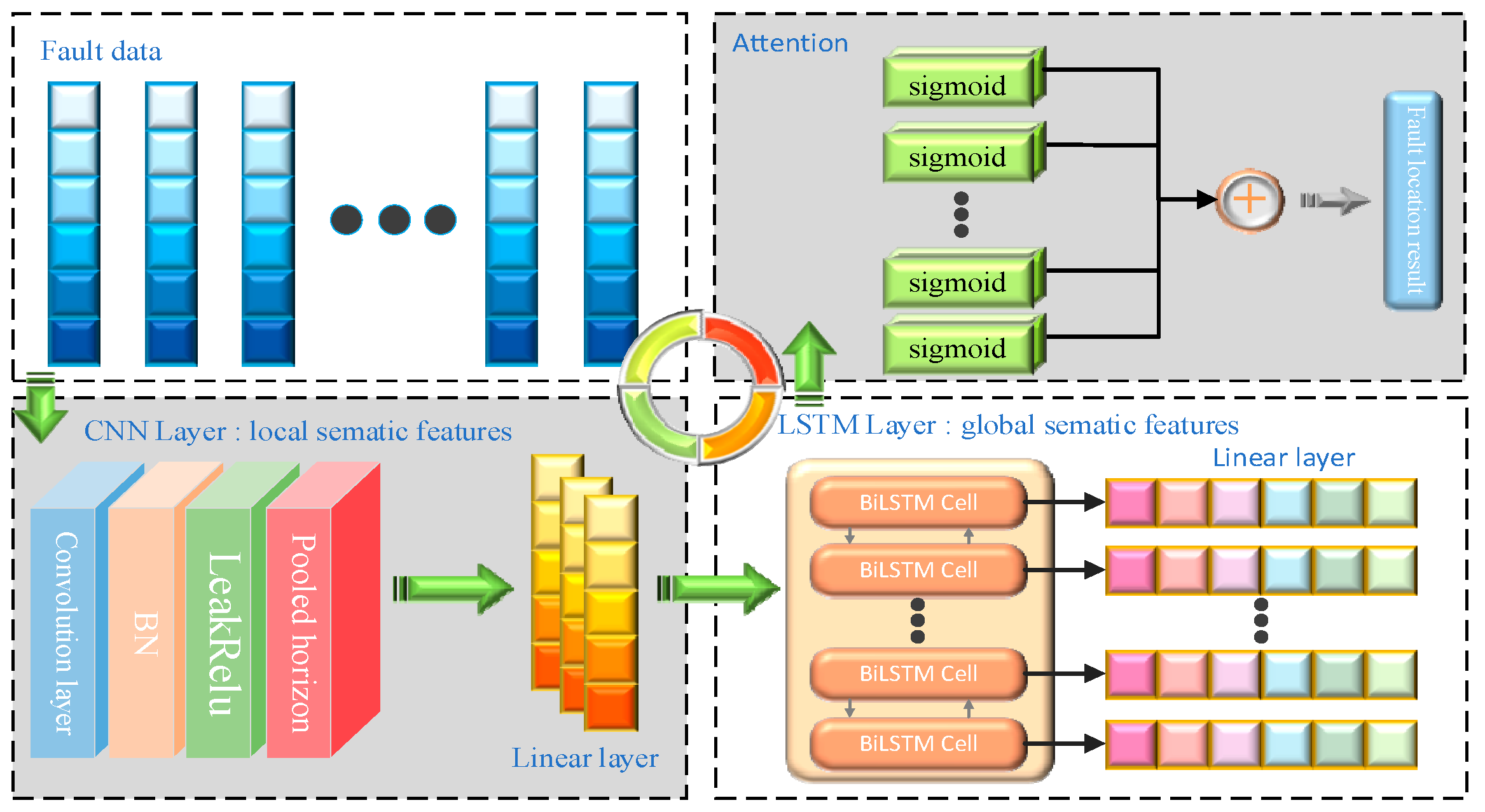
The CNN–BiLSTM–attention model operates through the coordinated integration of three core modules: (1) a convolutional neural network (CNN) for the extraction of spatial features from the input data; (2) a bidirectional long short-term memory (BiLSTM) network—comprising forward and backward LSTM layers—to capture bidirectional temporal dependencies and address challenges associated with long sequence modeling; and (3) an attention mechanism that assigns adaptive weights to the BiLSTM outputs, thereby emphasizing salient temporal features. This architecture effectively combines the spatial feature extraction capabilities of the CNN, the contextual modeling strength of BiLSTM, and the feature selection advantage of the attention mechanism, resulting in significant improvements in model accuracy and fault localization performance [24]. The overall model architecture is illustrated in Figure 5.

Fault Location Process of CNN–BiLSTM–Attention Model

The steps for the model to achieve more accurate fault location are as follows.

(1)

Fault sample data collection:

First, we build the wind farm simulation model as shown in Figure 1 in MATLAB. At the busbar of the wind farm (node A), at the connection of the overhead line and cable line (nodes B, C……) J, K), and at the connection of the fan to the line (nodes B’, C’…), zero-sequence current detection points are set for both J’ and K’. We set up a simulated fault point at different intervals on each cable line or overhead line, with a total of 20 simulated fault points. At each simulated fault location, batch simulations are conducted by configuring three-phase single-phase grounding faults with varying transition resistances and fault distances. Dedicated current sensors acquire zero-sequence signals, enabling the compilation of a comprehensive zero-sequence fault characteristic database.

(2)

Data extraction and preprocessing:

Firstly, the collected zero-sequence current, voltage, and three-phase waveforms are extracted from SIMULINK using the To Workspace component to the working area of MATLAB. Fast Fourier transform (FFT) spectral analysis quantifies both the fundamental amplitudes (three-phase current/voltage, zero-sequence current) and harmonic constituents within the three-phase electrical parameters. Given the significant dimensional heterogeneity and magnitude disparities among fault characteristic variables within wind farm collector systems, min–max normalization is implemented to standardize the parameters to the [0, 1] range, ensuring the equitable processing of the variable impacts on fault distance estimation.

$$x^{\prime }={\displaystyle \frac{x-x_{\min }}{x_{\max }-x_{\min }}}$$

(7)

Within the above equation, x denotes the measured fault data values from wind farm samples. x_min, x_max are, respectively, the minimum and maximum values of the corresponding columns of the characteristic variables.

For the tensor format data that the CNN can directly process, and for each sample, the branch label where the fault is located and the location label of the fault point are, respectively, obtained to form a fault data sample set that is easy to update and reuse. The complete dataset undergoes randomized partitioning into training, validation, and test subsets following an 8:1:1 allocation ratio.

(3)

Designing the structure of the CNN–BiLSTM–attention model:

A custom single-input dual-output CNN–BiLSTM–attention model is proposed, in which the output layer comprises two parallel multi-task classifiers for branch identification (classification) and fault distance estimation (regression). Task-specific loss functions are employed, and the model is trained on appropriately sized datasets with tuned iteration counts until convergence is achieved on the validation set, completing the offline training phase.

The training procedure includes the following: the CNN first performs local feature extraction and dimensionality reduction on the input data. Convolutional layers capture spatial patterns, followed by nonlinear activation and max-pooling operations to enhance feature abstraction and reduce redundancy. These representations serve as input to the BiLSTM module, which models temporal dependencies in both the forward and backward directions.

An attention mechanism is introduced within the BiLSTM hidden layers to dynamically reweight the contributions of time-step features. By adjusting the gate weights and biases through forward- and backpropagation, the model emphasizes informative temporal segments and mitigates issues such as vanishing gradients and output generalization.

Model performance is validated on the test dataset. The classification accuracy is used to assess branch-level fault identification, while the fault location precision is evaluated using the mean squared error (MSE), mean absolute error (MAE), and mean absolute percentage error (MAPE) metrics [25].

This article selects three evaluation indicators, which are specifically defined as follows.

(1)

The MSE quantifies the prediction accuracy through the arithmetic mean of the squared deviations between the model outputs $\overline{l_{\mathrm{i}\_\mathrm{pred}}}$ and observed values $l_{\mathrm{i}\_\mathrm{real}}$, and it is mathematically defined as

$$\mathrm{MSE}={\displaystyle \frac{1}{\mathrm{n}}}{{\displaystyle {\displaystyle \sum _{i=1}^n(l_{\mathrm{i}\_\mathrm{real}}-\overline{l_{\mathrm{i}\_\mathrm{pred}}}})}}^2$$

(8)

In the formula, $\overline{l_{\mathrm{i}\_\mathrm{pred}}}$ is the predicted fault distance; $l_{\mathrm{i}\_\mathrm{real}}$ represents the actual fault distance; and n is the number of samples in the test set.

(2)

The mean absolute error (MAE) is the average value of the absolute error between the predicted value and the true value, with the formula

$$\mathrm{MAE}={\displaystyle \sum _{i=1}^n\left|l_{\mathrm{i}\_\mathrm{real}}-\overline{l_{\mathrm{i}\_\mathrm{pred}}}\right|}$$

(9)

(3)

The mean absolute percentage error (MAPE) is the mean of the percentage of the absolute error to the true value and is given by the formula

$$\mathrm{MAPE}={\displaystyle \frac{100\%}{n}}{\displaystyle \sum _{i=1}^n\left|\frac{l_{\mathrm{i}\_\mathrm{real}}-\overline{l_{\mathrm{i}\_\mathrm{pred}}}}{l_{\mathrm{i}\_\mathrm{real}}}\right|}$$

(10)

(4)

Online fault location:

Firstly, the CNN–BiLSTM–attention hybrid model trained offline is invoked to load various weights and bias term parameters. Then, the fault samples obtained from the online fault data after data preprocessing are input into the model. Based on the nonlinear mapping relationship learned by the model, the fault branches and fault distances are predicted. The accurate location of the fault point is comprehensively obtained.

4. Simulation Verification

4.1. Construction of the Wind Farm Model and Generation of the Dataset

Taking a certain 35 kV wind farm as an example, the system built based on the MATLAB/SIMULINK platform has one feeder, and each feeder has two branches. The power generated by each wind turbine is collected on the collection line and connected to the 35 kV low-voltage busbar of the step-up substation through cables. Figure 4 shows a typical connection method for the collection lines in a wind farm. The wind turbine transformer and the system’s high-voltage components employ delta (Δ) connections, effectively isolating collector circuits from zero-sequence signal interference between the wind turbines and the transmission network. Given the △ configuration’s inability to suppress fault current flows via the main transformer’s neutral, Z-type grounding transformer installation becomes essential for bus voltage stabilization. The wind farm operational parameters are tabulated in

Table 2. Parameters of the wind farm model.

Name	Parameter Setting
Voltage level	35 kV
Transformer connection method	Yg-D1
Frequency	50 Hz

.

Table 3. Fault parameters.

Parameter	Numerical Value	Quantity
Fault type	AG, BG, CG	3
Transition resistor/Ω	0.001, 0.01, 0.05, 0.1, 1, 10, 100, 200	8
Initial phase angle/(°)	1.5, 30, 60, 90, 181.5, 210, 240, 270	8

comprehensively details the fault parameters characterizing the complete sample set. By permutation and combination, all fault parameters are traversed. There are a total of 20 simulated fault points, and all combinations have three types, $C_3^1{C}_3^1{C}_8^1{C}_8^1{C}_{20}^1$ (three types of ground faults, three types of single-phase ground faults occurring simultaneously, eight different transition resistors, eight types of initial phase angles of faults, and twenty simulated fault points). The total number of fault samples is 11,520, among which there are 1152 test set samples and 805 samples with transition resistance of 200 Ω. There are 288 samples with an initial phase angle of 1.5° or 181.5° for faults. The testing framework rigorously evaluates the proposed method’s ability to address weak fault conditions, including high-resistance ground faults and zero-crossing proximal faults. This experimental design accurately emulates the stochastic characteristics of practical fault occurrences.

4.2. Experimental Results and Analysis

4.2.1. Characteristic Analysis of Grounding Faults in a Single Line

During fault incidents along the C-C’ line, detection systems monitor the three-phase current waveforms in the affected branch alongside variations in the zero-sequence current and voltage parameters.

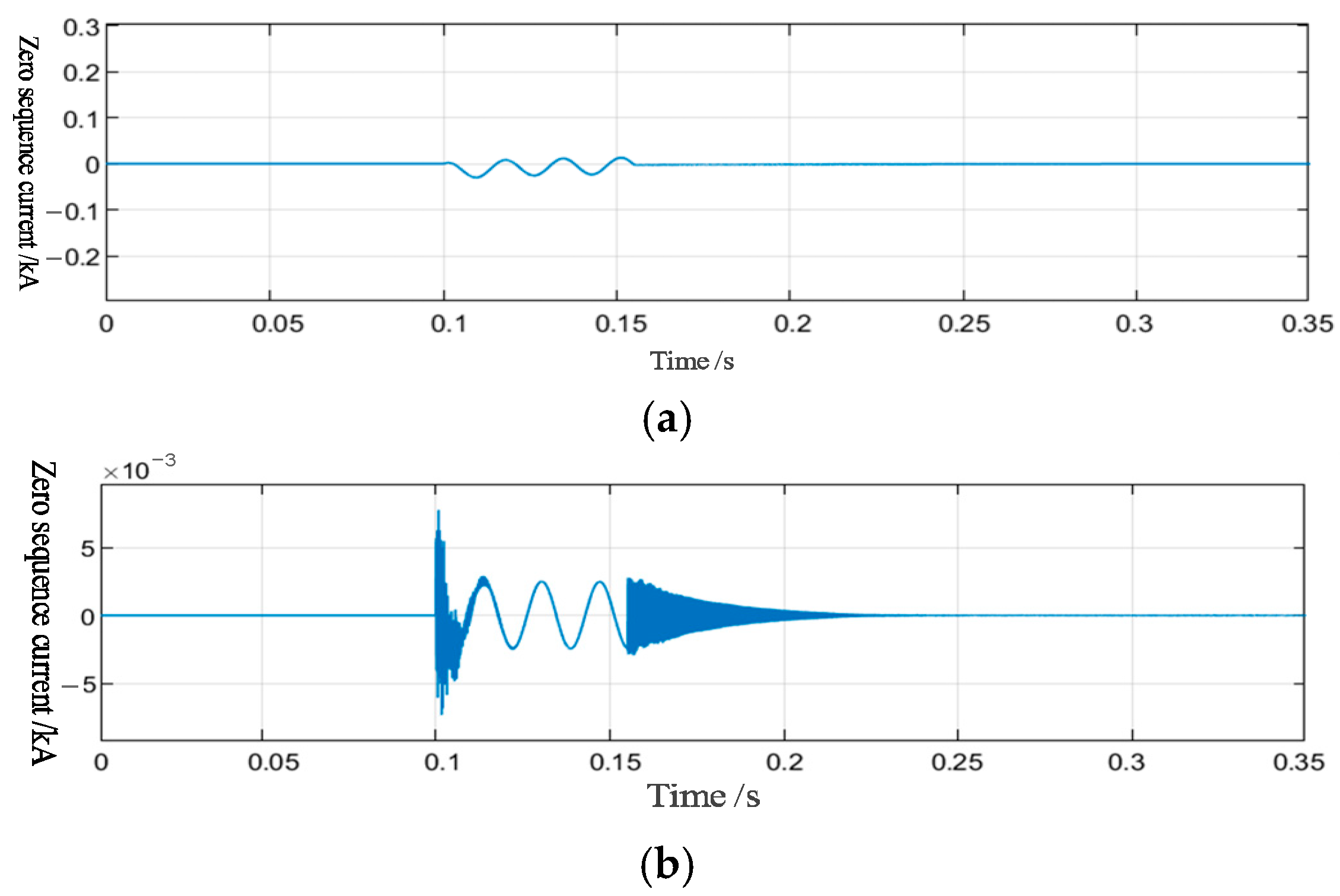
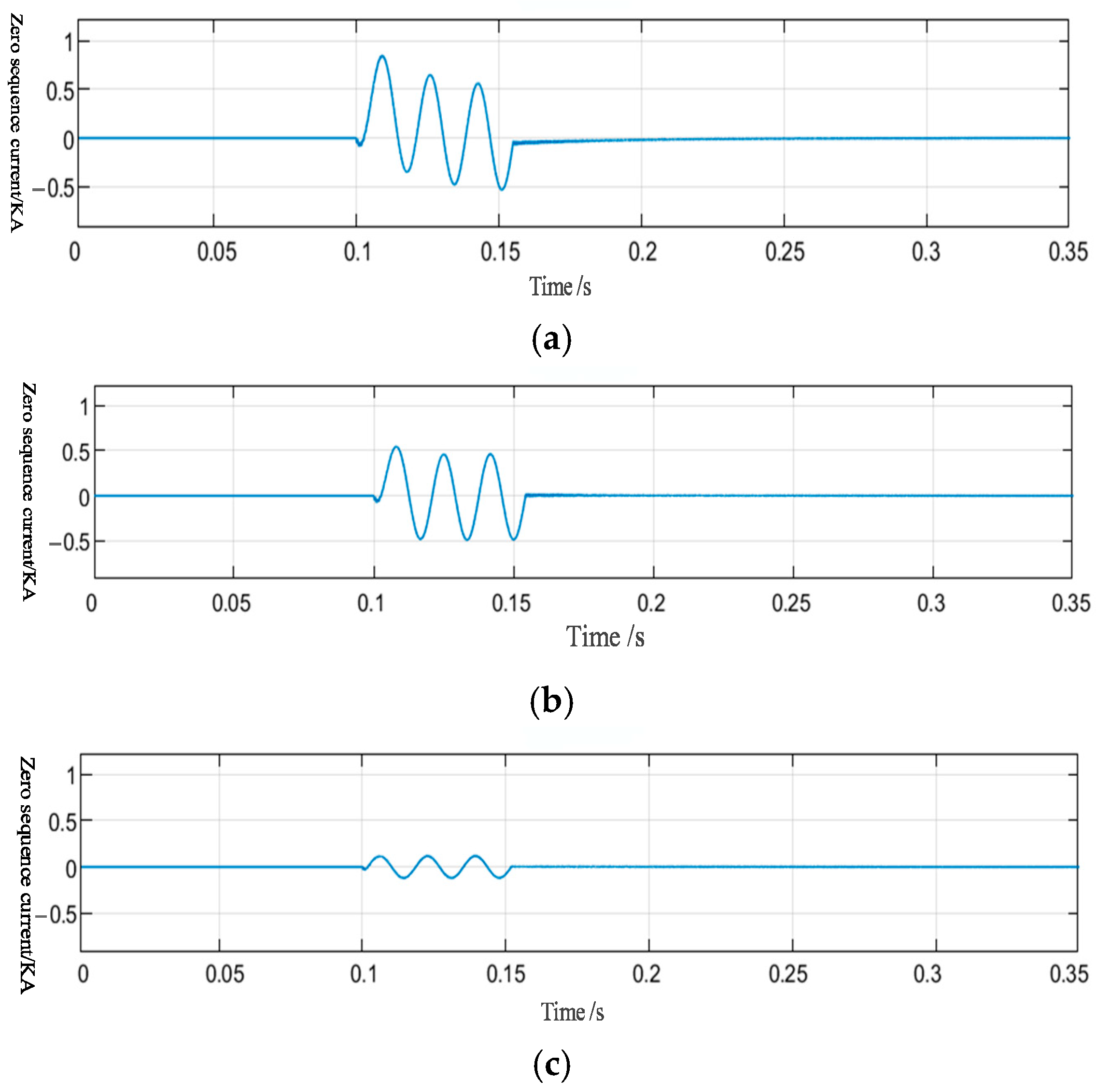
Figure 6 demonstrates that single-phase-to-ground faults produce a zero-sequence current and voltage with significant magnitude disparities. During normal operation (absence of grounding faults), the zero-sequence current remains absent, enabling its effective utilization as a reliable fault localization indicator.

A comparative analysis of Figure 6 and Figure 7 reveals a positive correlation between the proximity to the fault location and the measured zero-sequence parameter magnitude (current/voltage), demonstrating enhanced detection sensitivity near ground fault points.

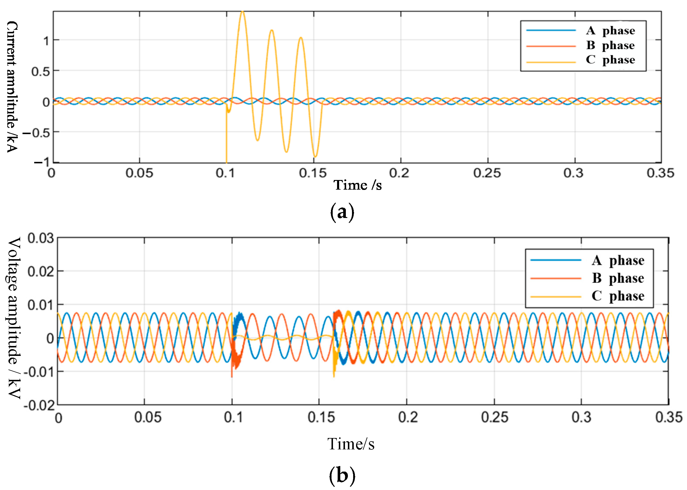
Figure 8 illustrates that three-phase-to-ground faults induce the highest amplitude volatility in the barrier current, while the affected phase voltage collapses to near-zero levels.

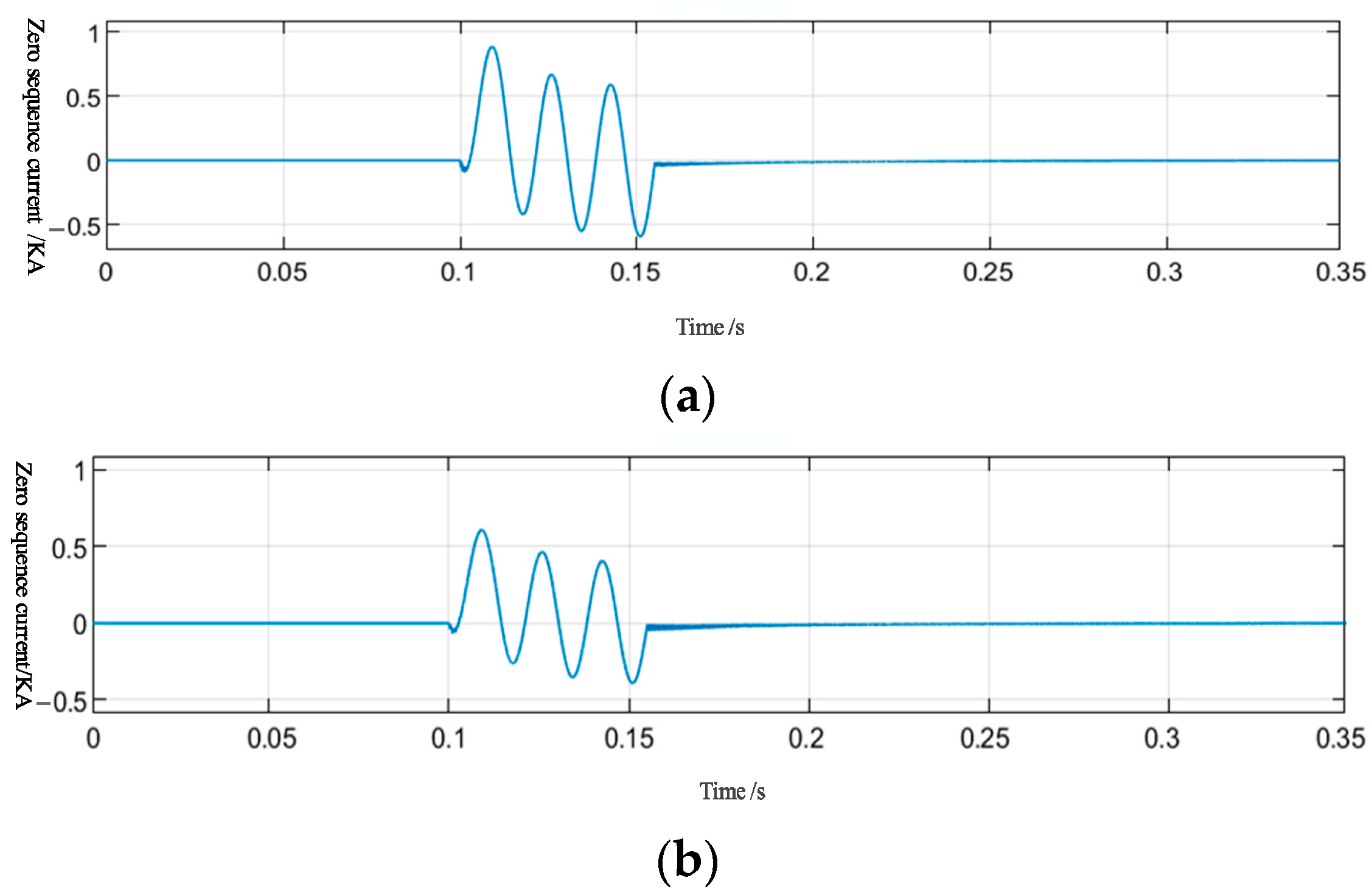
To validate the proposed feature vector construction method’s capacity to characterize fault distance variations, four test cases with C-phase ground faults (1 Ω grounding resistance) at 13 km and 25 km distances are analyzed. Figure 9 illustrates the corresponding zero-sequence current waveforms measured at monitoring point A across these fault distances.

Figure 9 reveals variations in the zero-sequence current waveform of the fault that correlate with fault distance progression. Therefore, the proposed feature extraction method can extract information about the fault location.

We use C-phase grounding faults with different resistance values (0.1 Ω, 10 Ω, 100 Ω) at a 13 km fault distance as a case study. Figure 10 depicts the zero-sequence current waveform variations across distinct grounding resistance conditions.

Figure 10 demonstrates that variations in grounding resistance directly influence the evolution of the fault’s zero-sequence current waveform.

4.2.2. Characteristic Analysis of Simultaneous Grounding Faults in Different Lines

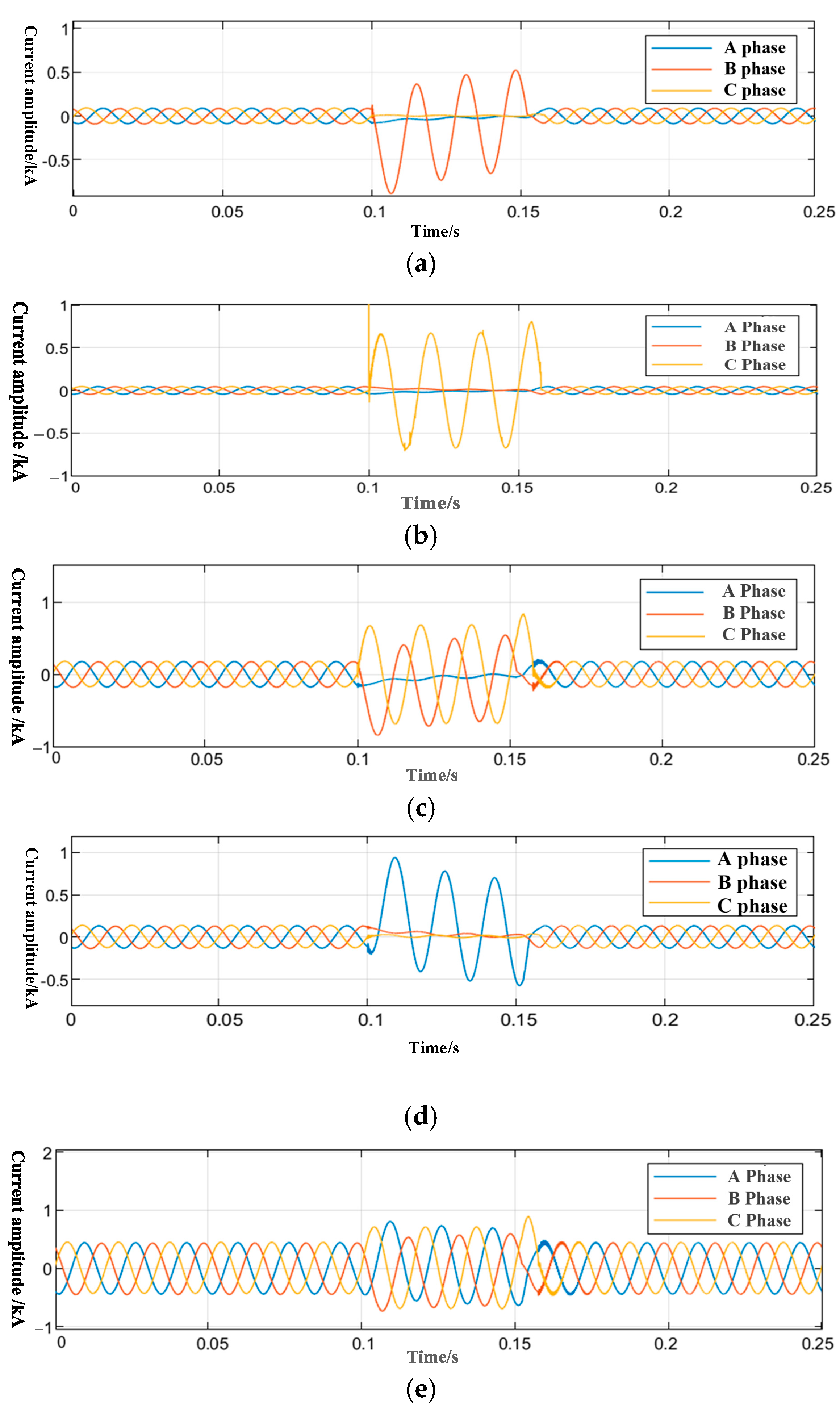
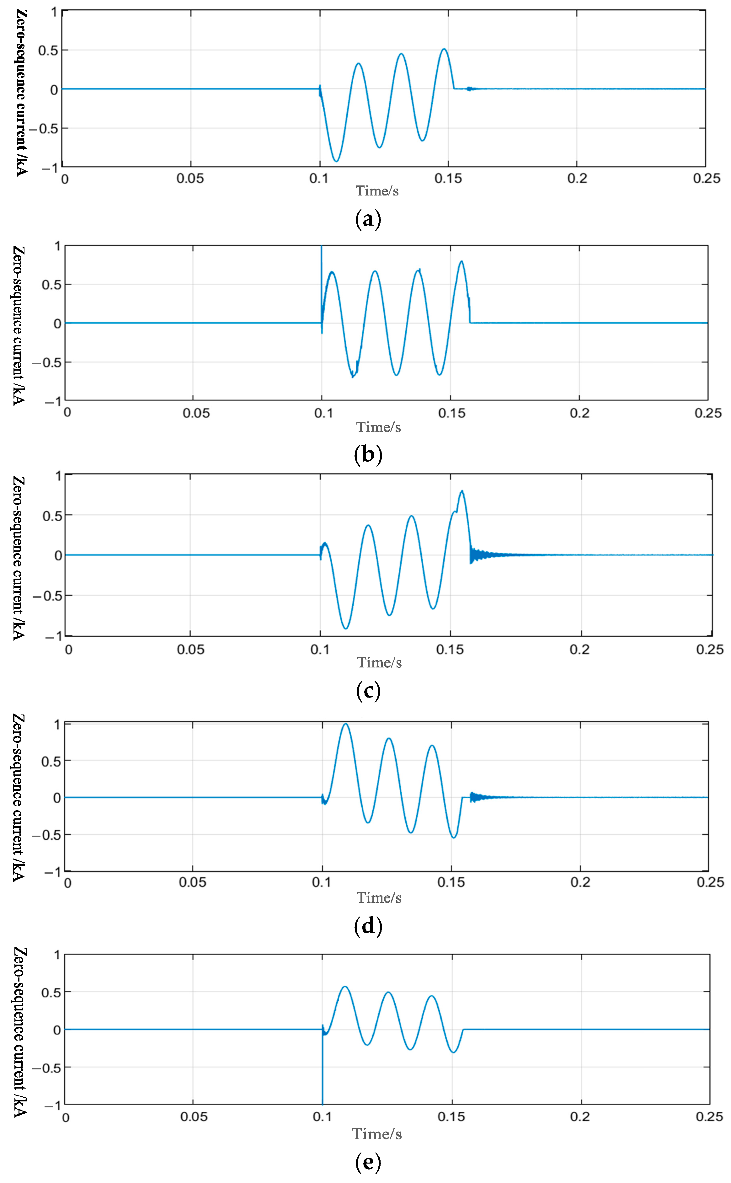
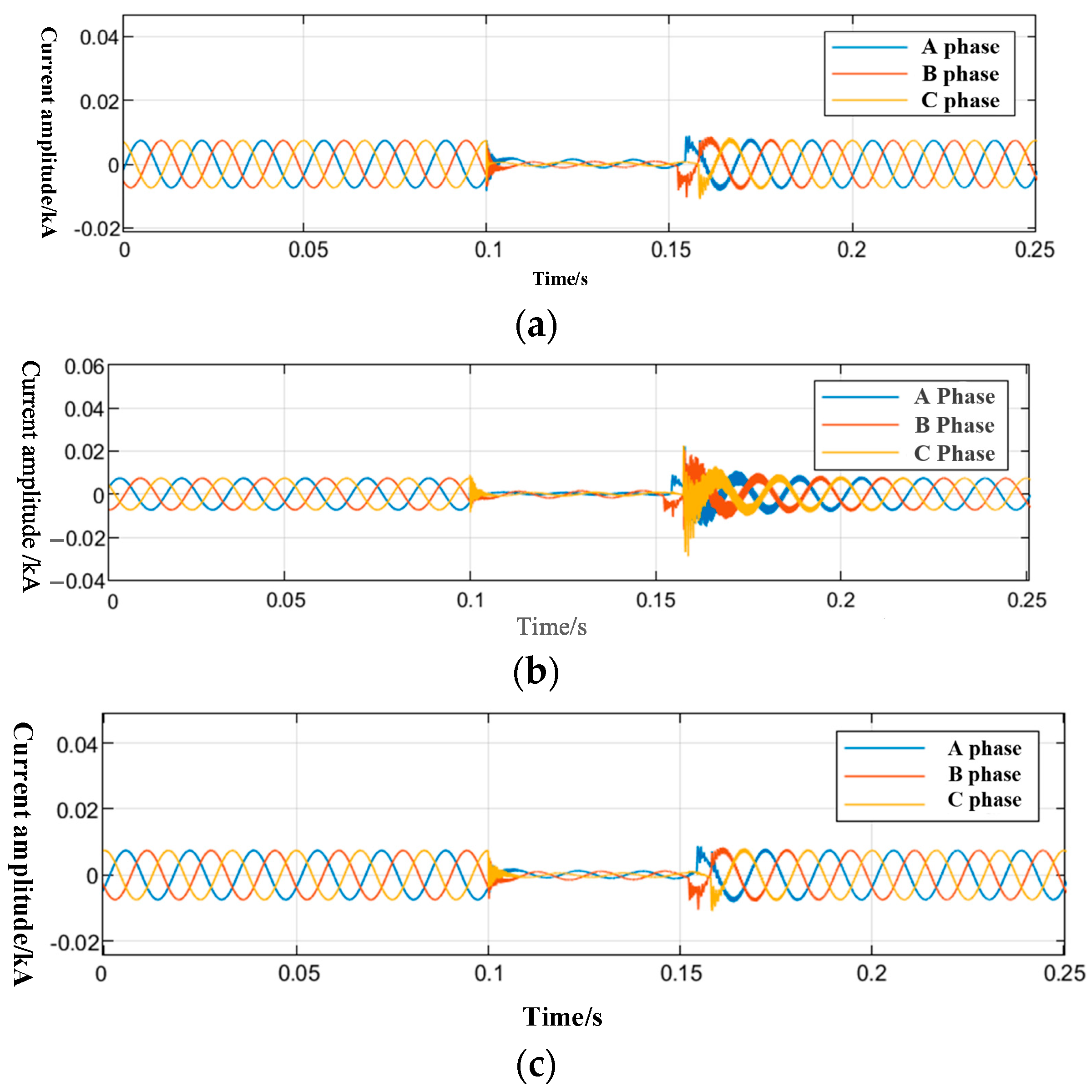
Experiment: The lines with simultaneous grounding faults and the fault phases are as follows: C-C’ line + C phase, E-E’ line + B phase, and I-I’ line + A phase. The location of the device for the detection of faults remains unchanged. The detection of the faulty branch’s three-phase current waveforms is performed, along with monitoring variations in the zero-sequence current and voltage parameters.

It can be seen from Figure 11 that the fault three-phase waveforms measured at point C are the superposition of the fault waveforms of the C-C’ line and the E-E’ line. Similarly, the three-phase fault waveforms measured at point A are the superposition of all the fault waveforms in this experiment.

It can be seen from Figure 12 that the zero-sequence current waveform measured at point C is the superposition of the fault waveforms of the C-C’ line and the E-E’ line. The fault three-phase waveform measured at point A is the superposition of all the fault waveforms in this experiment, which is the same as in the three-phase current fault waveform.

It can be seen from Figure 13 that the voltage waveforms of different faults occurring simultaneously on different lines are almost consistent and are not affected by the location and distance of the fault.

4.3. Fault Location Results Under Different Conditions

Given the predominance of overhead lines within the wind farm’s collector network, this investigation emulates single-phase-to-ground faults specifically along the D-D’ transmission segment. Localization inaccuracies derived from zero-sequence current methodologies are quantitatively evaluated in Figure 14.

Figure 14 demonstrates that the developed methodology achieves minimal localization errors in wind farm collector line fault detection while enabling precise fault point identification. To investigate the impact of varying short-circuit resistance values on the fault localization accuracy during short-circuit events, this study employs a simulation model to analyze single-phase ground faults across a range of short-circuit resistance conditions. The fault location results are shown in

Table 4. Ranging results of different transition resistors at the same fault point.

Actual Fault Distance/km	Ground Resistance/Ω	Calculated Distance/km	Absolute Error/km	Percentage Error
3.5	0.001	3.512	0.029	0.829%
	0.01	3.487	0.043	1.23%
	0.05	3.534	0.074	2.10%
	0.1	3.479	0.061	1.74%
	1	3.448	0.084	2.41%
	10	3.425	0.100	2.86%
	100	3.607	0.116	3.32%

.

The results in Table 4 show that the size of the grounding resistance has a certain influence on the result of fault location. Judging from the trend of change, as the grounding resistance gradually increases, the nonmetallic property becomes stronger, and the accuracy of fault location decreases. However, the error is still within 200 m, and relatively accurate fault location results can still be obtained.

4.4. Fault Location of CNN–BiLSTM–Attention

To validate the fault localization efficacy of the CNN–BiLSTM–attention architecture, this study employs MATLAB-generated wind farm model fault data as the primary experimental dataset.

After the fault features are extracted by the mutual information method, the key features are selected as input, and the CNN–BiLSTM–attention model is trained and optimized. The model parameter settings are shown in

Table 5. Information of model parameters.

Model Structure	Argument	Value
CNN layer	Window size	48
	Convolution kernel	128
	Convolution kernel 2	64
	Maximum pooling length	2
BiLSTM layer	BiLSTM unit 1	128
	BiLSTM unit 2	64
Fully connected layer	Output layer	One-dimensional vector
Dropout layer		Parameter: 0.2
Learning rate		0.001

.

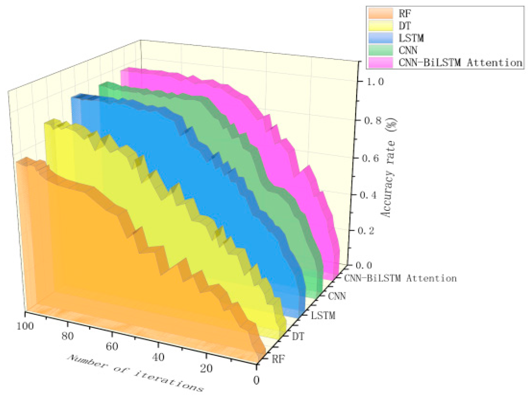
The dataset is partitioned into training, validation, and test subsets with an 8:1:1 allocation ratio. We compare the proposed CNN–BiLSTM–attention fusion model with a decision tree (DT), random forest (RF), LSTM, and the CNN. The same fault data are used to train the model and verify its accuracy, and the fault location results for different network test sets are shown in Figure 15.

Figure 15 reveals a progressive accuracy improvement across models with increasing iteration counts.

The CNN–BiLSTM–attention architecture achieves 98.96% precision at 59 iterations, demonstrating superior convergence speeds and stability. Comparatively, the LSTM model attains 97.15% accuracy after 63 iterations, followed by the CNN (95.97% at 66 iterations). Conventional methods show slower convergence: decision trees reach 82.83% at 79 iterations, while random forests plateau at 78.76% after 92 iterations. These results quantitatively confirm the proposed model’s enhanced fault localization capabilities.

4.5. Ablation Experiment

To investigate individual modules’ contributions in the fault localization framework, this study implements an ablation study framework comprising four architectures: CNN, BiLSTM, CNN–BiLSTM, and the novel CNN–LSTM configuration. The indicators described in Section 2.2 are used to measure the effects of different models, and the results are shown in

Table 6. Comparison of model results.

Model	MSE	MAE	MAPE
CNN	0.163	0.399	7.977%
BiLSTM	0.071	0.266	5.333%
CNN–BiLSTM–Attention	0.059	0.233	4.657%

.

The comprehensive analysis demonstrates the CNN–BiLSTM–attention architecture’s superior capabilities in extracting critical fault features from complex datasets. Furthermore, this architecture achieves enhanced localization precision compared to the benchmark models, exhibiting a 12.7% accuracy improvement over conventional approaches.

5. Conclusions

Leveraging the variation patterns of the line zero-sequence current, this study develops a hybrid fault localization framework that synergistically integrates a CNN, BiLSTM, and attention mechanisms. The model performance is quantified using three key metrics—the mean absolute percentage error (MAPE), mean squared error (MSE), and mean absolute error (MAE). The experimental results confirm the architecture’s effectiveness in identifying zero-sequence current dynamics, demonstrating superior positioning accuracy compared to conventional approaches.

An in-depth examination of the relationship between the zero-sequence current and line electrical parameters demonstrates that the grounding resistance and connection configuration predominantly govern this current’s behavioral characteristics. The research results in this paper are helpful in accurately identifying the requirements of fault points and have certain practical significance for the rapid and efficient operation and maintenance of wind farms.

References

1. Li, Z.; Ye, Y.; Ma, X.; Lin, X.; Xu, F.; Wang, C.; Ni, X.; Ding, C. Single-phase-to-ground fault section location in flexible resonant grounding distribution networks using soft open points. Int. J. Electr. Power Energy Syst. 2020, 122, 106198. [Google Scholar] [CrossRef]
2. Li, Z.; Wheeler, P.; Watson, A.; Costabeber, A.; Wang, B.; Ren, Y. A Fast Diagnosis Method for Both IGBT Faults and Current Sensor Faults in Grid-Tied Three-Phase Inverters with Two Current Sensors. IEEE Trans. Power Electron. 2020, 35, 5267–5278. [Google Scholar] [CrossRef]
3. Amatare, S.; Ojo, A. Predicting Customer Churn in Telecommunication Industry Using Convolutional Neural Network Model. IOSR J. Comput. Eng. 2021, 22, 54–59. [Google Scholar]
4. Belagoune, S.; Bali, N.; Bakdi, A.; Baadji, B.; Atif, K. Deep Learning through LSTM Classification and Regression for Transmission Line Fault Detection, Diagnosis and Location in Large-Scale Multi-Machine Power Systems. Measurement 2021, 177, 109330. [Google Scholar] [CrossRef]
5. Wang, X.; Zhou, P.; Peng, X.; Wu, Z.; Yuan, H. Fault location of transmission line based on CNN-LSTM double-ended combined model. Energy Rep. 2022, 8, 781–791. [Google Scholar] [CrossRef]
6. Zhang, J.; Ye, L.; Lai, Y. Stock Price Prediction Using CNN-BiLSTM-Attention Model. Mathematics 2023, 11, 1985. [Google Scholar] [CrossRef]
7. Zhang, F.; Liu, Q.; Liu, Y.; Tong, N.; Chen, S.; Zhang, C. Novel Fault Location Method for Power Systems Based on Attention Mechanism and Double Structure GRU Neural Network. IEEE Access 2020, 8, 75237–75248. [Google Scholar] [CrossRef]
8. Chen, W.; Song, H.; Wu, H.; Tian, H.; Qi, Z. Neural network based on hybrid ac/dc hybrid power grid ac line fault location. J. Sichuan Electr. Power Technol. 2024, 47, 66–75. [Google Scholar]
9. Yuan, S. Research on Single-Phase Grounding Short-Circuit Fault Location Method of Wind Farm Collector Line Based on Zero Sequence Network. Master’s Thesis, North China Electric Power University, Beijing, China, 2021; pp. 1–30. [Google Scholar]
10. Peng, H. Wind Power Electricity Lines of Single-Phase Grounding Fault Location Method Research. Ph.D. Thesis, North China Electric Power University, Beijing, China, 2022; pp. 1–24. [Google Scholar]
11. Liu, F.; Renna, S.; Zhu, Y. Location of single-phase grounding fault section of wind farm collector wire based on FDM twin network. Renew. Energy 2023, 41, 401–410. [Google Scholar]
12. Li, Z.; Zeng, X.; Xia, Y.; Wang, S.; Xi, Y. High voltage transmission line traveling wave fault location technology review. J. Chang. Univ. Sci. Technol. (Nat. Sci. Ed.) 2022, 19, 104–121. [Google Scholar]
13. Huang, W. Fault Diagnosis Method of NPC-Type Three-Level Grid-Connected Inverter Based on Observer. Master’s Thesis, Hefei University of Technology, Hefei, China, 2023; pp. 1–25. [Google Scholar]
14. Yang, L. Research on anomaly detection Algorithm of SCADA System based on Deep learning. Inf. Technol. Informatiz. 2024, 9–12. [Google Scholar]
15. Zhao, J.; Hou, H.; Gao, Y.; Huang, Y.; Gao, S.; Lou, J. Single-phase ground fault location method for distribution network based on traveling wave time-frequency characteristics. Electr. Power Syst. Res. 2020, 186, 106401. [Google Scholar]
16. Liang, J.; Jing, T.; Niu, H.; Wang, J. Two-terminal fault location method of distribution network based on adaptive convolution neural network. IEEE Access 2020, 8, 54035–54043. [Google Scholar] [CrossRef]
17. Wang, J.; Zhang, Y. Traveling wave propagation characteristic-based LCC-MMC hybrid HVDC transmission line fault location method. IEEE Trans. Power Deliv. 2021, 37, 208–218. [Google Scholar] [CrossRef]
18. Jalalt, S.M.; Miralizadeh, S.; Talavat, V.; Boalndi, T.G. A novel superimposed voltage energy-based approach for single phase to ground fault detection and location in distribution networks. IET Gener. Transm. Distrib. 2023, 17, 4215–4233. [Google Scholar] [CrossRef]
19. Tavoosi, J.; Shirkhani, M.; Azizi, A.; Din, S.U.; Mohammadzadeh, A.; Mobayen, S. A hybrid approach for fault location in power distributed networks: Impedance-based and machine learning technique. Electr. Power Syst. Res. 2022, 210, 108073. [Google Scholar] [CrossRef]
20. Lu, D.; Liu, Y.; Liao, Q.; Wang, B.; Huang, W.; Xi, X. Time-domain transmission line fault location method with full consideration of distributed parameters and line asymmetry. IEEE Trans. Power Deliv. 2020, 35, 2651–2662. [Google Scholar] [CrossRef]
21. Xu, L.; Fan, S.; Zhang, H.; Xiong, J.; Liu, C.; Mo, S. Enhancing Resilience and Reliability of Active Distribution Networks through Accurate Fault Location and Novel Pilot Protection Method. Energies 2023, 16, 7547. [Google Scholar] [CrossRef]
22. Shu, H.; Liu, X.; Tian, X. Single-ended fault location for hybrid feeders based on characteristic distribution of traveling wave along a line. Ower Delivery. IEEE Trans. Power Deliv. 2020, 36, 339–350. [Google Scholar] [CrossRef]
23. Dong, J.; Zhu, Y.; Cui, N.; Jia, X.; Guo, L.; Qiu, R.; Shao, M. Estimating crop evapotranspiration of wheat-maize rotation system using hybrid convolutional bidirectional Long Short-Term Memory network with grey wolf algorithm in Chinese Loess Plateau region. Agric. Water Manag. 2024, 301, 108924. [Google Scholar] [CrossRef]
24. Lu, G.; Liu, Y.; Wang, J.; Wu, H. CNN-BiLSTM-Attention: A multi-label neural classifier for short texts with a small set of labels. Inf. Process Manag. 2023, 60, 103320. [Google Scholar] [CrossRef]
25. Huang, Y.; Zhang, Z.; Chen, Q.; Liu, X.; Tu, J. CNN-BiLSTM Audible Noise Prediction for high-altitude multi-factor transmission lines based on multi-head attention mechanism. High Volt. Electr. Appar. 2024, 60, 160–169. [Google Scholar]
Figure 1. Schematic diagram of wind farm fault. Energies 18 03703 i001 indicates the system side; Energies 18 03703 i002 indicates the main transformer; Energies 18 03703 i003 indicates the grounding transformer.
Energies 18 03703 g001
Figure 2. The zero-sequence current flow direction diagram of the wind farm fault.
Energies 18 03703 g002
Figure 3. Simplified model of zero-order network in wind farms.
Energies 18 03703 g003
Figure 4. Flowchart of fault current location.
Energies 18 03703 g004
Figure 5. CNN–BiLSTM–attention hybrid neural network model.
Energies 18 03703 g005
Figure 6. Zero-sequence waveform of fault point. (a) Zero-sequence current waveform. (b) Zero-sequence voltage waveform.
Energies 18 03703 g006
Figure 7. Zero-sequence waveform measured at point B’. (a) Zero-sequence current waveform. (b) Zero-sequence voltage waveform.
Energies 18 03703 g007
Figure 8. Three-phase waveform measured at the fault point. (a) Three-phase current waveform. (b) Three-phase voltage waveform.
Energies 18 03703 g008
Figure 9. Zero-sequence current at different fault distances. (a) The fault distance is 13 km. (b) The fault distance is 25 km.
Energies 18 03703 g009
Figure 10. Zero-sequence current at different ground resistances. (a) The ground resistance is 0.1 Ω. (b) The ground resistance is 10 Ω. (c) The ground resistance is 100 Ω.
Energies 18 03703 g010
Figure 11. The three-phase current waveforms at each measurement point. (a) The waveform at point E. (b) The waveform at point C’. (c) The waveform at point C. (d) The waveform at point I. (e) The waveform at point A.
Energies 18 03703 g011
Figure 12. The zero-sequence current waveforms at each measurement point. (a) The waveform at point E. (b) The waveform at point C’. (c) The waveform at point C. (d) The waveform at point I. (e) The waveform at point A.
Energies 18 03703 g012
Figure 13. The three-phase voltage waveforms at each measurement point. (a) The waveform at point C. (b) The waveform at point I. (c) The waveform at point A.
Energies 18 03703 g013
Figure 14. Positioning errors at different fault distances.
Energies 18 03703 g014
Figure 15. Accuracy of different models.
Energies 18 03703 g015