A Ladder-Type Carbon Trading-Based Low-Carbon Economic Dispatch Model for Integrated Energy Systems with Flexible Load and Hybrid Energy Storage Optimization

Abstract

This paper proposes a ladder carbon trading-based low-carbon economic dispatch model for integrated energy systems (IESs), incorporating flexible load optimization and hybrid energy storage systems consisting of battery and thermal energy storage. First, a ladder-type carbon trading mechanism is introduced, in which the carbon trading cost increases progressively with emission levels, thereby providing stronger incentives for emission reduction. Second, flexible loads are categorized and modeled as shiftable, transferable, and reducible types, each with distinct operational constraints and compensation mechanisms. Third, both battery and thermal energy storage systems are considered to improve system flexibility by storing excess energy and supplying it when needed. Finally, a unified optimization framework is developed to coordinate the dispatch of renewable generation, gas turbines, waste heat recovery units, and multi-energy storage devices while integrating flexible load flexibility. The objective is to minimize the total system cost, which includes energy procurement, carbon trading expenditures, and demand response compensation. Three comparative case studies are conducted to evaluate system performance under different operational configurations: the proposed comprehensive model, a carbon trading-only approach, and a conventional baseline scenario. Results demonstrate that the proposed framework effectively balances economic and environmental objectives through coordinated demand-side management, hybrid storage utilization, and the ladder-type carbon trading market mechanism. It reshapes the system load profile via peak shaving and valley filling, improves renewable energy integration, and enhances overall system efficiency.

1. Introduction

With the global emphasis on sustainable development and the urgent need to mitigate climate change, integrated energy systems (IESs) have emerged as a promising approach by harmonizing electricity, heat, and gas networks to optimize energy structure, enhance energy efficiency, and promote the consumption of renewable energy.

Many studies have explored optimal scheduling strategies for IESs, with a focus on economic efficiency, operational safety, and renewable energy integration [1,2,3]. However, as carbon reduction targets become increasingly stringent, cost-centric dispatch models are no longer adequate. Environmental impacts should be integrated into operational planning [4]. The low-carbon potential of IESs remains underutilized. Carbon trading provides a market-based solution by assigning costs to emissions, encouraging energy producers to reduce their emissions by imposing costs on carbon output. Traditional carbon trading mechanisms often apply a uniform price, lacking the granularity to incentivize deeper emission cuts. A ladder-type carbon trading mechanism, where pricing tiers escalate with emission levels, can more effectively drive low-carbon transitions [5,6,7]. The core feature of the ladder-type carbon trading mechanism is to divide carbon emissions into multiple tiers, each with a different carbon trading price. This creates progressive cost pressure and encourages enterprises to actively reduce carbon emissions. The ladder-type carbon pricing mechanism has gained increasing attention due to its intuitive structure and strong incentive effect on emission reduction. In [8], a robust optimal dispatch strategy for a park-level IES, considering a ladder-type carbon trading mechanism, is proposed to guide the IES to control carbon emissions. Reference [9] developed a meteorological classification-based robust dispatch strategy for multi-microgrid systems, combining wind pattern clustering, data augmentation, ladder-type carbon trading, and distributed optimization to address wind power uncertainty while ensuring low-carbon and economical operation. Reference [10] proposed an integrated demand response exchange mechanism for coordinated low-carbon dispatch in electricity–gas systems, combining emission reduction valuation, game-theoretic market clearing, and CCPP-P2G synergy to incentivize decarbonization while enhancing economic efficiency. Reference [11] introduced a ladder-type carbon trading mechanism based on the Chinese Certified Emission Reduction (CCER) quota system, focusing on capacity configuration and lifecycle cost optimization. It employs sensitivity analysis to determine the carbon trading parameters.

Traditionally, loads in integrated energy systems are treated as inflexible and uncontrollable. With the development of smart grid technologies, flexible loads—such as shiftable, transferable, and reducible electricity and heat demands—can now play a significant role in balancing supply and demand, smoothing load profiles, and improving the efficiency of resource allocation [12,13]. Reference [14] proposed an equivalent aggregation method for large-scale flexible loads in power systems, clustering them into parameter-based groups to create simplified equivalent models that enable efficient peak shaving and valley filling in system scheduling while maintaining accuracy and computational speed. In [15], a method for the economic dispatch of a park-level integrated energy system that considers the characteristics of flexible loads and variable operating conditions of equipment is proposed. Reference [16] proposed a robust optimization model for CHP demand response that integrates flexible electric and thermal loads to enhance peak regulation capacity while addressing uncertainties in wind power and load response. Reference [17] developed a two-stage stochastic optimization model for integrated energy system planning that incorporates flexible thermal/electrical loads and auxiliary devices. Reference [18] proposed a distributed low-carbon scheduling model for park-level integrated energy systems that combines game-theoretic energy sharing, improved Shapley value-based benefit allocation, and integrated demand response to enhance renewable utilization, economic efficiency, and fair profit distribution while ensuring privacy protection. Reference [19] developed a low-carbon dispatch framework for integrated energy systems by synergizing carbon capture technology with power-to-gas conversion, introducing carbon-aware energy storage management, and implementing incentive-based demand response while utilizing a parallel multi-dimensional dynamic programming algorithm to efficiently address operational uncertainties. Reference [20] proposed a source-load coordinated low-carbon economic dispatch model for multi-energy virtual power plants, integrating organic Rankine cycle waste heat recovery and comprehensive demand response to enhance flexibility, improve carbon capture efficiency, and balance economic and environmental objectives in system operation. Reference [21] proposed a low-carbon hierarchical demand response framework for power systems, integrating carbon flow tracking and multi-source-grid-load coordination to optimize resource allocation and enhance the system’s low-carbon economic operation.

Although increasing attention has been given to the economic and low-carbon dispatch of integrated energy systems (IESs), several key challenges remain. In particular, the modeling and scheduling of flexible loads are often simplified or aggregated in existing studies without distinguishing between different types of demand-side flexibility. This limits the accuracy of dispatch outcomes and reduces the potential of flexible loads in supporting renewable energy integration and carbon emission reduction. To address this, a detailed modeling framework for flexible loads is proposed in this paper, in which loads are classified into three categories—shiftable, transferable, and reducible—each with specific operational constraints and corresponding compensation mechanisms. This classification allows for more effective use of demand-side resources and enhances system flexibility. A low-carbon economic dispatch model is formulated, integrating renewable energy sources, gas turbines, waste heat recovery units, flexible loads, and hybrid energy storage systems composed of both battery and thermal energy storage. The objective function minimizes the total system cost, including electricity purchases, carbon trading expenses, and demand response payments. A ladder-type carbon trading mechanism is introduced to calculate the carbon trading cost, in which the carbon trading cost increases progressively with emission levels, thereby providing stronger incentives for emission reduction. Sensitivity analysis is conducted to determine appropriate values for the key parameters of the carbon trading mechanism. Finally, three comparative case studies are presented to evaluate system performance under different configurations. Scenario 1 represents the proposed model, which incorporates both the ladder-type carbon trading mechanism and flexible load optimization. Scenario 2 considers a dispatch model that includes only the ladder-type carbon trading mechanism. Scenario 3 serves as the baseline model, excluding both carbon trading and flexible load optimization.

The remainder of this paper is organized as follows. Section 2 details the IES structure and the ladder-type carbon trading mechanism. Section 3 presents the optimization model, including objective functions and constraints. Section 4 analyzes simulation results across scenarios. Section 5 presents the conclusions and future directions.

2. IES Structure and Ladder-Type Carbon Trading Mechanism

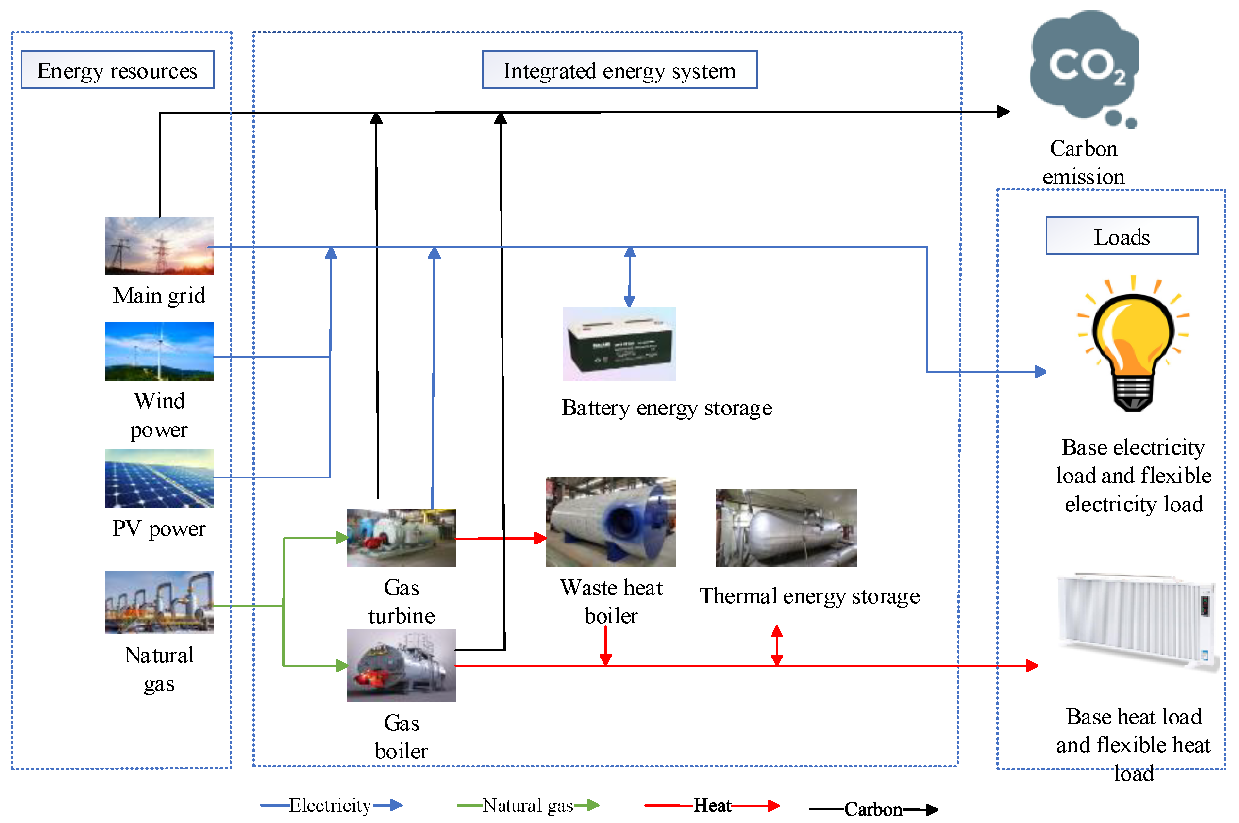
2.1. Structure of the IES

The structure of the IES used in this paper is illustrated in Figure 1. Energy inputs are derived from the main power grid and the main gas network, as well as renewable energy sources such as solar and wind power. Energy conversion devices include gas turbines (GTs), gas boilers (GBs), and waste heat boilers (WHBs). There exist both battery energy storage and thermal energy storage systems. The load side includes electrical and thermal loads, and they are categorized into base loads and flexible loads, which can participate in demand response. In this paper, it is considered that all electricity purchased by the IES from the grid is produced by thermal power plants. Therefore, for the IES, there are three sources of carbon emissions: purchased electricity, gas turbines, and gas boilers. The difference between the IES’s actual carbon emissions and carbon credit allowances is traded through the carbon trading market using a ladder-type carbon trading mechanism.

2.2. Carbon Credit Allowance Calculation Model

Carbon trading is a mechanism for achieving carbon emissions control by creating legal carbon credits and allowing them to be traded. The government or regulator allocates free carbon credit allowances based on the total amount of energy consumed or power generated by each emission source. If emissions exceed their allowances, they need to purchase additional ones in the carbon trading market; conversely, if emissions are lower than the allowances, they can sell the excess emission allowances in the market and obtain the corresponding revenue. Therefore, the ladder-type carbon trading mechanism mainly consists of three parts: the carbon credit allowances, the actual carbon emissions, and the cost of laddered carbon trading. The carbon credit allowance calculating model used in this paper is as follows [22]:

$$\{\begin{array}{l}{E}_{IES}=E_{buy}+E_{GT}+E_{GB}\\ E_{buy}={\theta }_e{\displaystyle \sum _{t=1}^{NT}{P}_t^{grid}}\\ E_{GT}={\theta }_h{\displaystyle \sum _{i=1}^{NGT}{\displaystyle \sum _{t=1}^{NT}({\partial }_{e,h}{P}_{i,t}^{gt}+H_{i,t}^{gt})}}\\ E_{GB}={\theta }_h{\displaystyle \sum _{i=1}^{NGB}{\displaystyle \sum _{t=1}^{NT}{H}_{i,t}^{\mathrm{gb}}}}\end{array}$$

(1)

where $E_{IES}$ is the total carbon credit allowances of the IES; $E_{buy}$, $E_{GT}$, and $E_{GB}$ are the carbon credit allowances of the purchased electricity, gas turbines, and gas boilers, respectively; $P_t^{grid}$ denotes the amount of active power purchased from the power grid during time period $t$; ${\theta }_e$ and ${\theta }_h$ are carbon emission allowances per unit of electrical power and per unit of thermal power generation, respectively; ${\partial }_{e,h}$ is the efficiency with which electrical energy is converted to heat; $P_{i,t}^{gt}$ is the electric power generated by GT; $H_{i,t}^{gt}$ is the exhaust heat power recovery of GT; $H_{i,t}^{gb}$ is the heat power generated by GB; $NGT$ and $NGB$ represent the number of units for gas turbines and gas boilers, respectively.

2.3. Actual Carbon Emissions Calculation Model

The carbon emissions calculation model used in this paper is as follows:

$$\{\begin{array}{l}{E}_{IESa}=E_{buya}+E_{GTa}+E_{GBa}\\ E_{buya}={\chi }_e{\displaystyle \sum _{t=1}^{NT}{P}_t^{grid}}\\ E_{GTa}={\chi }_h{\displaystyle \sum _{i=1}^{NGT}{\displaystyle \sum _{t=1}^{NT}({\partial }_{e,h}{P}_{i,t}^{gt}+H_{i,t}^{gt})}}\\ E_{GBa}={\chi }_h{\displaystyle \sum _{i=1}^{NGB}{\displaystyle \sum _{t=1}^{NT}{H}_{i,t}^{gb}}}\end{array}$$

(2)

where $E_{IESa}$ represents the total actual carbon emissions of the IES; $E_{buya}$ is the actual carbon emissions from main grid thermal units; $E_{MTa}$ and $E_{GBa}$ represent the actual carbon emissions from gas turbines and gas boilers, respectively; ${\chi }_e$ denotes carbon emissions per unit of electrical power generated; and ${\chi }_h$ denotes carbon emissions per unit of heat power generated.

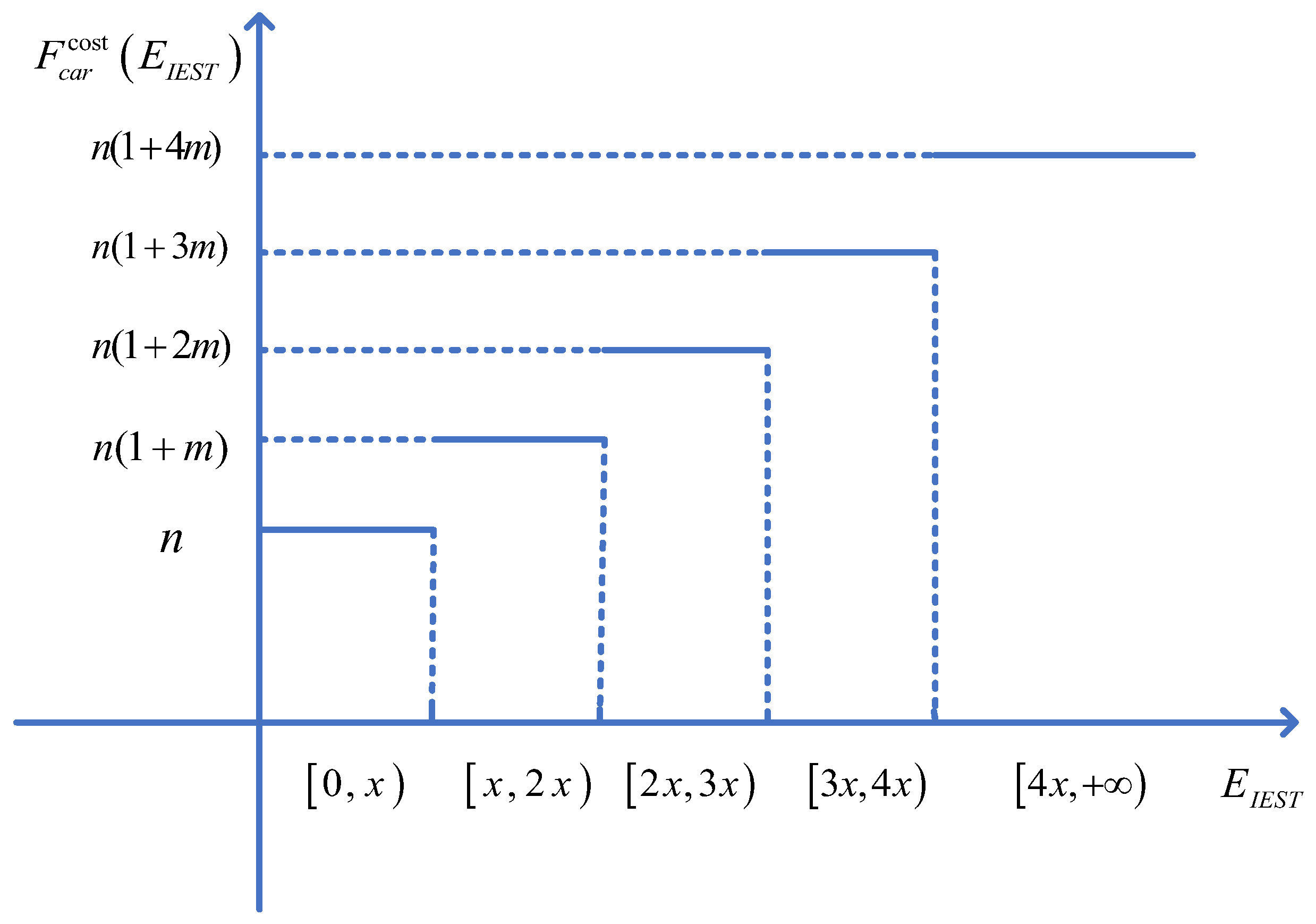
2.4. Ladder-Type Carbon Trading Mechanism

Based on the difference between the IES’s total actual carbon emissions and carbon credit allowances, the amount of carbon emissions for participation in the carbon trading market can be calculated as follows:

$$E_{IEST}=E_{IESa}-E_{IES}$$

(3)

Different from traditional carbon trading, the ladder-type carbon trading mechanism divides the price of carbon trading into multiple intervals in terms of the amount of carbon emissions traded in the IES, as shown in Figure 2.

$$F_{car}^{\mathrm{cost}}=\{\begin{array}{l}n{E}_{IEST},E_{IEST}\le x\\ n\left(1+m\right)\left(E_{IEST}-x\right)+nx,x\le E_{IEST}\le 2x\\ n\left(1+2m\right)\left(E_{IEST}-2x\right)+n\left(2+m\right)x,2x\le E_{IEST}\le 3x\\ n\left(1+3m\right)\left(E_{IEST}-3x\right)+n\left(3+3m\right)x,3x\le E_{IEST}\le 4x\\ n\left(1+4m\right)\left(E_{IEST}-4x\right)+n\left(4+6m\right)x,4x\le E_{IEST}\end{array}$$

(4)

where $F_{car}^{\mathrm{cost}}$ is the carbon trading cost; $n$ is the carbon trading base price; $x$ is the length of the carbon trading interval; $m$ is the transaction price growth rate. These parameters can be determined through simulation-based sensitivity analysis by varying one parameter while fixing the other two.

3. Low-Carbon Economic Dispatch Optimization Model for the IES

3.1. Mathematical Models for Flexible Loads

The load types considered in this paper include base loads (i.e., uncontrollable loads) and flexible loads (i.e., controllable loads). According to the control methods of flexible loads, this paper categorizes flexible loads into three major types—shiftable loads, transferable loads, and reducible loads—and establishes mathematical models for each type of flexible load.

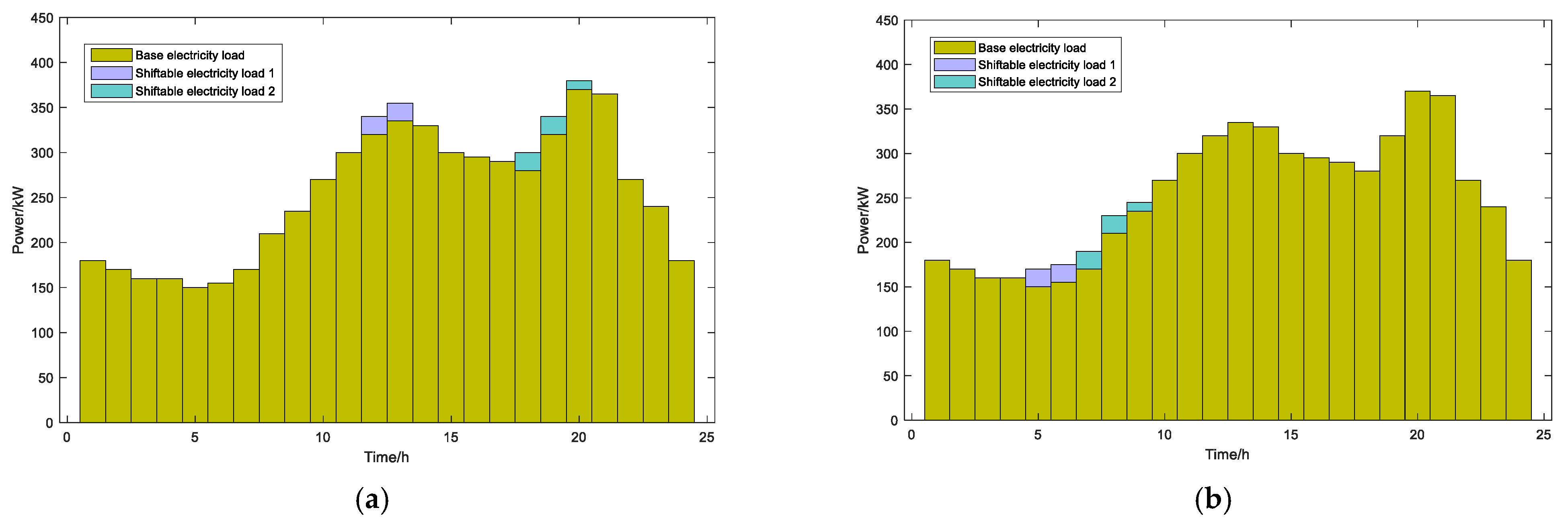
3.1.1. Shiftable Loads

A shiftable load refers to a load with constant power and a fixed duration of usage. When shifting, the entire load must be shifted as a whole, meaning its operating time can be adjusted, but it cannot be interrupted, and its power consumption remains unchanged during the shifting process.

To model shiftable loads, we first introduce a binary variable $u_{i,t}$ representing the shifting state (indicating whether shiftable load $i$ starts shifting at time period $t$) and a variable $P_{i,t}^{sh,aft}$ representing the load power of shiftable load $i$ at time period $t$. Then, based on the original load power $P_{i,t}^{sh,org}$ of the shiftable load in each time period, the original operating time range $\left[t_{i,-}^{sh,org},t_{i,+}^{sh,org}\right]$, and the acceptable shifting time range $\left[t_{i,-}^{sh,acp},t_{i,+}^{sh,acp}\right]$, the shiftable load model is constructed, including its constraints and objective function. The mathematical model is as follows:

$$\{\begin{array}{l}{u}_{i,t}=0,\hspace{1em}\hspace{1em}\hspace{1em}\hspace{1em}t\notin \left[t_{i,-}^{sh,acp},t_{i,+}^{sh,acp}-t_{i,+}^{sh,org}+t_{i,-}^{sh,org}\right]\\ 0\le {\displaystyle \sum _{z=t_{i,-}^{sh,acp}}^{t_{i,+}^{sh,acp}-t_{i,+}^{sh,org}+t_{i,-}^{sh,org}}{u}_{i,z}\le 1},\hspace{1em}\hspace{1em}\hspace{1em}t\in \left[t_{i,-}^{sh,acp},t_{i,+}^{sh,acp}-t_{i,-}^{sh,org}+t_{i,+}^{sh,org}\right]\\ P_{i,t}^{sh,aft}=(1-{\displaystyle \sum _{z=t_{i,-}^{sh,acp}}^{t_{i,+}^{sh,acp}-t_{i,+}^{sh,org}+t_{i,-}^{sh,org})}{u}_{i,z})P_{i,t}^{sh,bef}},\hspace{1em}t\notin \left[t_{i,-}^{sh,acp},t_{i,+}^{sh,acp}\right]\\ P_{i,t}^{sh,aft}={\displaystyle \sum _{z=t_{i,-}^{sh,acp}}^t{u}_{i,z}{P}_{i,t-z+t_{i,-}^{sh,org}}^{sh,org}},\hspace{1em}\hspace{1em}\hspace{1em}t\in \left[t_{i,-}^{sh,acp},t_{i,+}^{sh,acp}\right]\end{array}$$

(5)

$$F_{sh}^{\mathrm{cost}}=C_{sh,t}{\displaystyle \sum _{i=1}^{NSH}{\displaystyle \sum _{z=t_{i,-}^{sh,acp}}^{t_{i,+}^{sh,acp}-t_{i,+}^{sh,org}+t_{i,-}^{sh,org}}{u}_{i,z}}}({\displaystyle \sum _{t=t_{i,-}^{sh,org}}^{t_{i,+}^{sh,org}}{P}_{i,t}^{sh,org}\Delta t)}$$

(6)

In Equation (6), $F_{sh}^{\mathrm{cost}}$ represents the compensation cost for shiftable load scheduling; $C_{sh,t}$ denotes the unit energy shifting compensation cost at time period $t$; $NSH$ is the number of shiftable loads.

Since a shiftable load can be shifted at most once, it can only start shifting at a single time period within the acceptable shifting time range. Therefore, $0\le {\displaystyle \sum _{z=t_{i,-}^{sh,acp}}^{t_{i,+}^{sh,acp}-t_{i,+}^{sh,org}+t_{i,-}^{sh,org}}{u}_{i,z}\le 1},\hspace{1em}t\in \left[t_{i,-}^{sh,acp},t_{i,+}^{sh,acp}-t_{i,-}^{sh,org}+t_{i,+}^{sh,org}\right]$. The third and fourth equations in (5) indicate that if the load is shifted (i.e., ${\displaystyle \sum _{z=t_{i,-}^{sh,acp}}^{t_{i,+}^{sh,acp}-t_{i,+}^{sh,org}+t_{i,-}^{sh,org}}{u}_{i,z}=1}$), then for time slots outside the acceptable shifting range (i.e., $t\notin \left[t_{i,-}^{sh,acp},t_{i,+}^{sh,acp}\right]$), the load power $P_{i,t}^{sh,aft}=0$, and for time slots inside the acceptable shifting range (i.e., $t\in \left[t_{i,-}^{sh,acp},t_{i,+}^{sh,acp}\right]$), the load power at the shifted starting time equals the original power at the initial operating time $t_{i,-}^{sh,org}$, and the power at the subsequent time slot equals the original power at $t_{i,-}^{sh,org}+1$ and so on. If the load is not shifted, then the load power $P_{i,t}^{sh,aft}$ remains equal to the original load power $P_{i,t}^{sh,org}$. For example, consider a shiftable load with the following characteristics: original operating time range is [4, 6], and acceptable shifting time range is [10, 15]. The original load power vector is as follows:

$$P_i^{sh,org}=[0,0,0,P_{i,4}^{sh,org},P_{i,5}^{sh,org},P_{i,6}^{sh,org},0,0,\dots ,0]$$

(7)

According to the fourth equation in (5), when $t$ belongs to the acceptable translation range time period [10, 15], we have

$$\begin{array}{l}{P}_{i,10}^{sh,aft}=u_{i,10}{P}_{i,4}^{sh,org}\\ P_{i,11}^{sh,aft}=u_{i,10}{P}_{i,5}^{sh,org}+u_{i,11}{P}_{i,4}^{sh,org}\\ P_{i,12}^{sh,aft}=u_{i,10}{P}_{i,6}^{sh,org}+u_{i,11}{P}_{i,5}^{sh,org}+u_{i,12}{P}_{i,4}^{sh,org}\\ P_{i,13}^{sh,aft}=u_{i,10}{P}_{i,7}^{sh,org}+u_{i,11}{P}_{i,6}^{sh,org}+u_{i,12}{P}_{i,5}^{sh,org}+u_{i,13}{P}_{i,4}^{sh,org}\\ P_{i,14}^{sh,aft}=u_{i,10}{P}_{i,8}^{sh,org}+u_{i,11}{P}_{i,7}^{sh,org}+u_{i,12}{P}_{i,6}^{sh,org}+u_{i,13}{P}_{i,5}^{sh,org}+u_{i,14}{P}_{i,4}^{sh,org}\\ P_{i,15}^{sh,aft}=u_{i,10}{P}_{i,9}^{sh,org}+u_{i,11}{P}_{i,8}^{sh,org}+u_{i,12}{P}_{i,7}^{sh,org}+u_{i,13}{P}_{i,6}^{sh,org}+u_{i,14}{P}_{i,5}^{sh,org}+u_{i,15}{P}_{i,4}^{sh,org}\end{array}$$

(8)

Since there can only be one $u_{i,t}$ variable with a value of 1, each of the above equations can only be equal to one of the polynomials on the right. Assuming that $t=10$ the shiftable load $i$ starts to shift, then $u_{i,10}=1$, and the other time slots $u_{i,t}=0$, then it is as follows:

$$P_{i,10}^{sh,aft}=P_{i,4}^{sh,org},\hspace{1em}{P}_{i,11}^{sh,aft}=P_{i,5}^{sh,org},\hspace{1em}{P}_{i,12}^{sh,aft}=P_{i,6}^{sh,org},\hspace{1em}{P}_{i,13}^{sh,aft}=0,\hspace{1em}{P}_{i,14}^{sh,aft}=0,\hspace{1em}{P}_{i,15}^{sh,aft}=0$$

(9)

Equation (9) demonstrates that the operational time slot of the shiftable load has been rescheduled from hours 4–6 to hours 10–12, with the load power profile remaining unchanged. This example aligns with the mathematical model’s constraints and demonstrates how the formulation enforces feasible shifting behavior.

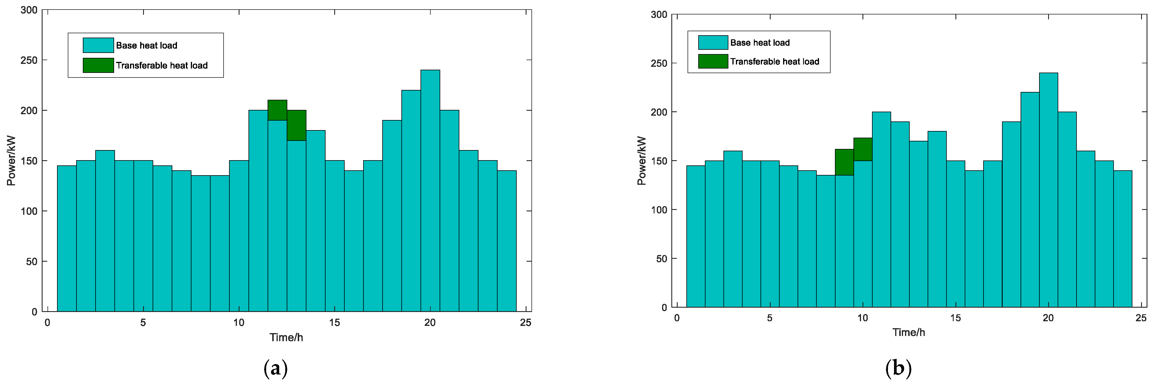
3.1.2. Transferable Loads

Transferable loads are not constrained by continuous operating time requirements, and their power consumption in each time period can be flexibly adjusted. However, the total power consumption before and after transfer must remain unchanged. To model transferable loads, we first define the following variables: binary operating state variable ${\beta }_{i,t}$ (indicating whether transferable load $i$ operates at time $t$, where ${\beta }_{i,t}=1$ denotes operation, and ${\beta }_{i,t}=0$ denotes non-operation) and load power variable $P_{i,t}^{tr,aft}$. Based on the original load power $P_{i,t}^{tr,org}$, the original operating time range $\left[t_{i,-}^{tr,org},t_{i,+}^{tr,org}\right]$, and the acceptable transfer time range $\left[t_{i,-}^{tr,acp},t_{i,+}^{tr,acp}\right]$, we construct the transferable load model, including its constraints and objective function. The mathematical formulation is as follows:

$$\{\begin{array}{l}{\beta }_{i,t}=0,t\notin \left[t_{i,-}^{tr,org},t_{i,+}^{tr,org}\right]\mathrm{U}\left[t_{i,-}^{tr,acp},t_{i,+}^{tr,acp}\right]\\ {\beta }_{i,t}{P}_i^{tr,\min }\le P_{i,t}^{tr,aft}\le {\beta }_{i,t}{P}_i^{tr,\max },t\in \left[t_{i,-}^{tr,org},t_{i,+}^{tr,org}\right]\mathrm{U}\left[t_{i,-}^{tr,acp},t_{i,+}^{tr,acp}\right]\\ {\displaystyle \sum _{t=1}^{NT}{P}_{i,t}^{tr,aft}}\Delta t={\displaystyle \sum _{t=1}^{NT}{P}_{i,t}^{tr,org}}\Delta t\end{array}$$

(10)

where $P_i^{tr,\min }$ and $P_i^{tr,\max }$ are the minimum and maximum operating power of transferable load $i$, respectively.

The first and second formulation in (10) indicate that when $t$ is within either the original or transferable time range, the load power can be adjusted—either set to zero or within the allowable power bounds $\left[P_i^{tr,\min },P_i^{tr,\max }\right]$. In other words, regardless of the original load power, the post-transfer load power can be increased or decreased, provided it remains within the permissible range. The third formulation ensures the total energy demand remains unchanged before and after transfer.

To formulate the compensation cost objective function for transferable load scheduling, we define the power adjustment variable $\Delta P_{i,t}^{tr}$ as follows:

$$\Delta P_{i,t}^{tr}=P_{i,t}^{tr,aft}-P_{i,t}^{tr,bef}$$

(11)

Since $\Delta P_{i,t}^{tr}$ can be positive or negative, we use its absolute value multiplied by time and unit energy compensation cost to construct the transferable load scheduling compensation cost $F_{tr}^{\mathrm{cost}}$ as follows:

$$F_{tr}^{\mathrm{cost}}={\displaystyle \sum _{i=1}^{NTR}{\displaystyle \sum _{t=1}^{NT}{C}_{tr,t}}\left|\Delta P_{i,t}^{tr}\right|}\Delta t$$

(12)

where $C_{tr.t}$ is the unit energy transfer compensation cost at time period $t$; $NTR$ is the number of transferable loads.

Since Equation (12) contains an absolute value (a nonlinear term), it is challenging to solve directly. To linearize it, we introduce an auxiliary variable $Y_{i,t}$ and reformulate the objective function as (13) while adding constraint set (14).

$$F_{tr}^{\mathrm{cost}}={\displaystyle \sum _{i=1}^{NTR}{\displaystyle \sum _{t=1}^{NT}{C}_{tr,t}{Y}_{i,t}}}\Delta t$$

(13)

$$\begin{array}{l}\Delta P_{i,t}^{tr}\le Y_{i,t}\\ -\Delta P_{i,t}^{tr}\le Y_{i,t}\\ 0\le Y_{i,t}\end{array}$$

(14)

This ensures both the objective function and constraints remain linear, facilitating efficient optimization.

This linearization is exact and widely accepted in mixed-integer linear programming (MILP). It introduces no relaxation or approximation as long as the deviation $\Delta P_{i,t}^{tr}$ is a linear function of the decision variables, which is the case in our model. Since the objective function minimizes $F_{tr}^{\mathrm{cost}}={\displaystyle \sum _{i=1}^{NTR}{\displaystyle \sum _{t=1}^{NT}{C}_{tr}{Y}_{i,t}}}\Delta t$ and the constraints enforce $Y_{i,t}\ge \left|\Delta P_{i,t}^{tr}\right|$, the optimizer will choose the smallest possible value of $Y_{i,t}$ that satisfies both $Y_{i,t}\ge \Delta P_{i,t}^{tr}$ and $Y_{i,t}\ge -\Delta P_{i,t}^{tr}$. This minimal feasible value is precisely as follows:

$$Y_{i,t}=\max \left\{\Delta P_{i,t}^{tr},-\Delta P_{i,t}^{tr}\right\}=\left|\Delta P_{i,t}^{tr}\right|$$

(15)

Thus, the auxiliary variable $Y_{i,t}$ exactly equals the absolute value of $\Delta P_{i,t}^{tr}$ at optimality. Therefore, the linearized formulation is mathematically equivalent to the original nonlinear form in the objective function and introduces no approximation or relaxation.

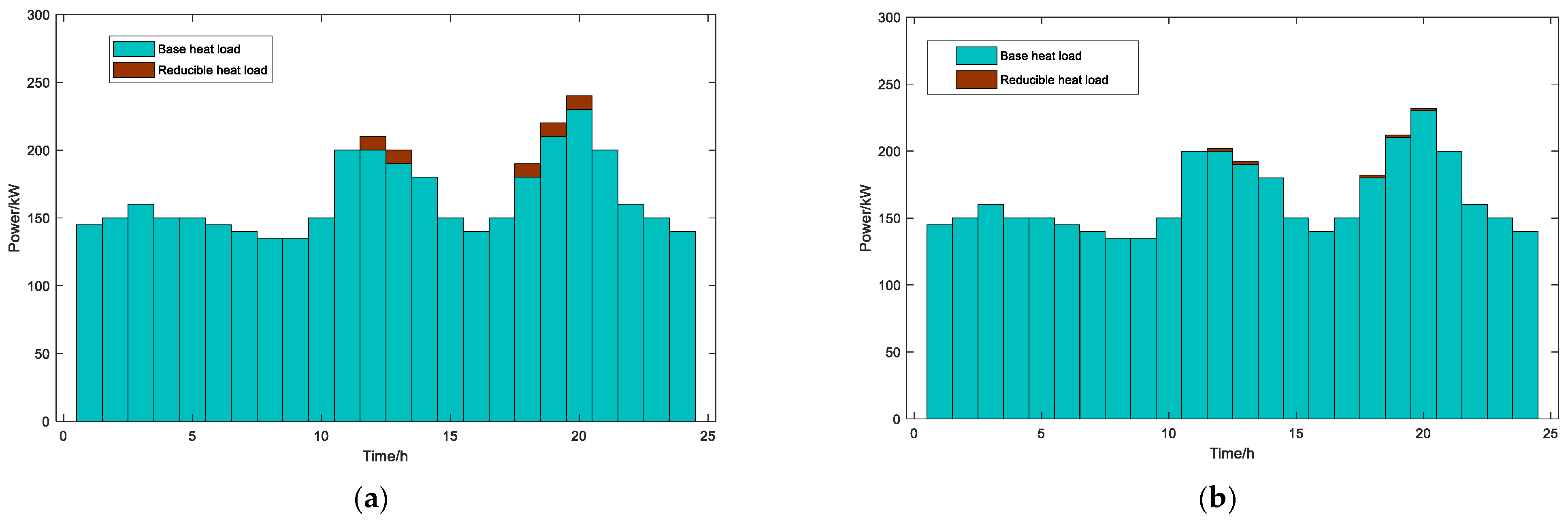
3.1.3. Reducible Loads

Reducible loads refer to those capable of enduring partial or complete interruptions or power reductions, allowing for adjustable operation time or power. To model reducible loads, we need a continuous variable $\Delta P_{i,t}^{cut}$ that represents the power reduction of a reducible load and a continuous variable $P_{i,t}^{cut,aft}$ that represents the load power after curtailment. These two variables are used to construct constraints and the compensation cost objective function for reducible loads. The mathematical formulation is as follows:

$$\begin{array}{l}{P}_{i,t}^{cut,aft}=P_{i,t}^{cut,org}-\Delta P_{i,t}^{cut}\\ 0\le \Delta P_{i,t}^{cut}\le {\theta }_i^{cut}{P}_{i,t}^{cut,org}\end{array}$$

(16)

$$F_{cut}^{\mathrm{cost}}=C_{cut,t}{\displaystyle \sum _{i=1}^{NCL}{\displaystyle \sum _{t=1}^{NT}\Delta P_{i,t}^{cut}}}\Delta t$$

(17)

where ${\theta }_i^{cut}$ is the maximum allowable percentage of load that can be curtailed; $P_{i,t}^{cut,org}$ is the original load power of reducible load $i$ at time slot $t$; $C_{cut,t}$ denotes the unit energy cutting compensation cost at time period $t$; $NCL$ is the number of reducible loads.

The preceding sections have presented the three categories of flexible electric load models proposed in this study. For flexible thermal loads, analogous operational models can be established using similar methodologies, which will not be elaborated here for brevity. Based on the three flexible load operation models established above, IES operators can optimize flexible load behaviors to reduce expense costs and promote renewable energy consumption.

It is important to acknowledge that the proposed mathematical models for flexible loads are developed based on several simplifying assumptions to maintain tractability. These load models assume ideal shifting, transferring, and curtailment of loads without accounting for user discomfort, time delays, or behavioral uncertainties. While such assumptions facilitate system-level analysis, they may not fully reflect practical demand-side flexibility in real-world scenarios. Future research can extend this framework by incorporating more detailed behavioral models, such as probabilistic user response functions or elasticity-based demand models. These enhancements would allow for a more accurate representation of load flexibility and provide deeper insights into the interaction between human behavior and energy system operation.

3.2. Mathematical Models for Battery Energy Storage and Thermal Energy Storage Systems

The operation constraints and objective function for battery energy storage systems are as follows:

$$\{\begin{array}{l}0\le {\alpha }_{i,t}^{cha}+{\alpha }_{i,t}^{dis}\le 1\\ {\alpha }_{i,t}^{cha}{P}_{i,\min }^{cha}\le P_{i,t}^{cha}\le {\alpha }_{i,t}^{cha}{P}_{i,\max }^{cha}\\ {\alpha }_{i,t}^{dis}{P}_{i,\min }^{dis}\le P_{i,t}^{dis}\le {\alpha }_{i,t}^{dis}{P}_{i,\max }^{dis}\\ SO{C}_{i,t}^e==SO{C}_{i,t-1}^e+{\displaystyle \frac{{\eta }_i^{cha}{P}_{i,t}^{cha}\Delta t}{E_{i,\max }^e}}-{\displaystyle \frac{P_{i,t}^{dis}\Delta t}{{\eta }_i^{dis}{E}_{i,\max }^e}}\\ SO{C}_{i,\min }^e\le SO{C}_{i,t}^e\le SO{C}_{i,\max }^e\\ SO{C}_{i,0}^e=SO{C}_{i,ini}^e\\ SO{C}_{i,NT}^e=SO{C}_{i,0}^e\end{array}$$

(18)

$$F_{eess}^{\mathrm{cost}}={\displaystyle \sum _{t=1}^{NT}{\displaystyle \sum _{i=1}^{NES}{C}_{ess}(P_{i,t}^{cha}+P_{i,t}^{dis})}}\Delta t$$

(19)

where ${\alpha }_{i,t}^{cha}$ and ${\alpha }_{i,t}^{dis}$ are the 0–1 variables representing the charging and discharging states of electricity energy storage system $i$ at time period $t$, respectively; $P_{i,t}^{cha}$ and $P_{i,t}^{dis}$ are the charging power and discharging power, respectively; $P_{i,\min }^{cha}$ and $P_{i,\max }^{cha}$ are the lower and upper limits of the charging power, respectively; $E_{i,\max }^e$ is the capacity of electricity energy storage system; ${\eta }_i^{cha}$ and ${\eta }_i^{dis}$ are the charging and discharging efficiencies, respectively; $E_{i,\min }^{bess}$ and $E_{i,\max }^{bess}$ are the lower and upper limits of the state of charge of electricity energy storage system; $SO{C}_{i,ini}^e$ is the initial state of charge; $F_{bess}$ is the operation cost of electricity energy storage system.

The operation constraints and objective function for thermal energy storage systems are as follows:

$$\{\begin{array}{l}0\le {\chi }_{i,t}^{cha}+{\chi }_{i,t}^{dis}\le 1\\ {\chi }_{i,t}^{cha}{H}_{i,\min }^{cha}\le H_{i,t}^{cha}\le {\chi }_{i,t}^{cha}{H}_{i,\max }^{cha}\\ {\chi }_{i,t}^{dis}{H}_{i,\min }^{dis}\le H_{i,t}^{dis}\le {\chi }_{i,t}^{dis}{H}_{i,\max }^{dis}\\ E_{i,t}^{hst}=E_{i,t-1}^{hst}(1-h_i^{loss})+(H_{i,t}^{cha}{\mu }_i^{cha}-{\displaystyle \frac{H_{i,t}^{dis}}{{\mu }_i^{dis}}})\Delta t\\ E_{i,\min }^{hst}\le E_{i,t}^{hst}\le E_{i,\max }^{hst}\\ E_{i,0}^{hst}=E_{i,ini}^{hst}\\ E_{i,NT}^{hst}=E_{i,0}^{hst}\end{array}$$

(20)

$$F_{hst}^{\mathrm{cost}}={\displaystyle \sum _{t=1}^{NT}{\displaystyle \sum _{i=1}^{NHST}{C}_{hst}(H_{i,t}^{cha}+H_{i,t}^{dis})}}\Delta t$$

(21)

where ${\chi }_{i,t}^{cha}$ and ${\chi }_{i,t}^{dis}$ are the 0–1 variables representing the charging and discharging states of the heat storage tank $i$ at time period $t$; $H_{i,\max }^{cha}$ and $H_{i,\min }^{cha}$ are the upper and lower charging power limits; $H_{i,\max }^{dis}$ and $H_{i,\min }^{dis}$ are the upper and lower limits of the discharge power; $E_{i,t}^{hst}$ is the heat energy stored in heat storage tank $i$ at time period $t$; $h_i^{loss}$ is the self-loss efficiency; ${\mu }_i^{cha}$ and ${\mu }_i^{dis}$ are the heat charging and discharging efficiencies, respectively; $E_{i,\max }^{hst}$ and $E_{i,\min }^{hst}$ are the upper and lower limits of the capacity; $E_{i,ini}^{hst}$ is the initial amount of energy stored in heat storage tank $i$ in initial time slot; $F_{hst}^{\mathrm{cost}}$ is the operation costs of the heat energy storage system.

It is worth noting that the model does not impose fixed priorities between the battery energy storage system and thermal energy storage system during the scheduling process. Instead, the optimization solver dynamically determines their charging and discharging schedules based on objective function and constraints, including electricity/gas price signals, renewable energy availability, heat/electricity load demand, carbon trading costs, and energy storage efficiencies. A key coordination mechanism lies in the charging/discharging cost coefficients of BESS and TES in the objective function. These coefficients directly influence their dispatch priorities. Under the premise of satisfying all the constraints, the storage system with a lower cost coefficient will be scheduled to charge or discharge preferentially.

3.3. Mathematical Models for GT, GB, WHB, and Wind and PV Power Generation Systems

The operation constraints and objective function for GT, WAB, and GB are as follows [23]:

$$F_{i,t}^{GT}={\displaystyle \frac{P_{i,t}^{gt}\Delta t}{{\eta }_i^{gte}{L}_{NG}}}$$

(22)

$$H_{i,t}^{gt}={\displaystyle \frac{P_{i,t}^{gt}}{{\eta }_i^{gte}}}\left(1-{\eta }_i^{gte}-{\eta }_i^{gtl}\right)$$

(23)

$$0\le H_{i,t}^{wab}\le {\eta }_i^{wab}{H}_{i,t}^{gt}$$

(24)

$$0\le H_{i,t}^{wab}\le H_{i,\max }^{wab}$$

(25)

$$P_{i,\min }^{gt}\le P_{i,t}^{gt}\le P_{i,\max }^{gt}$$

(26)

$$-\Delta P_{i,\max }^{gt,down}\le P_{i,t+1}^{gt}-P_{i,t}^{gt}\le \Delta P_{i,\max }^{gt,up}$$

(27)

$$F_{i,t}^{GB}={\displaystyle \frac{H_{i,t}^{gb}\Delta t}{{\eta }_i^{gb}{L}_{NG}}}$$

(28)

$$H_{i,\min }^{gb}\le H_{i,t}^{gb}\le H_{i,\max }^{gb}$$

(29)

$$F_{gas}^{\mathrm{cost}}={\displaystyle \sum _{t=1}^{NT}{C}_{gas}({\displaystyle \sum _{i=1}^{NGB}{F}_{i,t}^{GB}}+{\displaystyle \sum _{i=1}^{NGT}{F}_{i,t}^{GT}})}$$

(30)

where ${\eta }_i^{gte}$ is electric power generation efficiency coefficient of GT; $L_{NG}$ is the low calorific value of natural gas, which is typically 9.7 kWh/m³; ${\eta }_i^{gtl}$ is the heat dissipation loss coefficient; ${\eta }_i^{wab}$ denotes the heat recovery efficiency; $P_{i,\min }^{gt}$ and $P_{i,\max }^{gt}$ are the minimum and maximum electric power output of GT; $\Delta P_{i,\max }^{gt,down}$ and $\Delta P_{i,\max }^{gt,up}$ are the ramp-down and ramp-up rates of GT; ${\eta }_i^{gb}$ is heat power generation efficiency coefficient of GB; $H_{i,\min }^{gb}$ and $H_{i,\max }^{gb}$ are the minimum and maximum heat power output of GB; $F_{gas}$ is the cost of natural gas consumed by GB and GT; $C_{gas}$ is the price of natural gas per unit.

The operation constraints and objective function for wind and PV power generation systems are as follows:

$$0\le \Delta P_{i,t}^{wpc}\le P_{i,t}^{fwp}$$

(31)

$$P_{i,t}^{awp}=P_{i,t}^{fwp}-\Delta P_{i,t}^{wpc}$$

(32)

$$0\le \Delta P_{i,t}^{pvc}\le P_{i,t}^{fpv}$$

(33)

$$P_{i,t}^{apv}=P_{i,t}^{fpv}-\Delta P_{i,t}^{pvc}$$

(34)

$$F_{res,opr}^{\mathrm{cost}}={\displaystyle \sum _{t=1}^{NT}[{\displaystyle \sum _{i=1}^{NWP}\left(C_{wp}{P}_{i,t}^{awp}\Delta t\right)}+{\displaystyle \sum _{i=1}^{NPV}\left(C_{pv}{P}_{i,t}^{apv}\Delta t\right)}]}$$

(35)

$$F_{res,cut}^{\mathrm{cost}}={\displaystyle \sum _{t=1}^{NT}[{\displaystyle \sum _{i=1}^{NWP}\left(C_{wpc}\Delta P_{i,t}^{wpc}\Delta t\right)}+{\displaystyle \sum _{i=1}^{NPV}\left(C_{pvc}\Delta P_{i,t}^{pvc}\Delta t\right)}]}$$

(36)

where $P_{i,t}^{fwp}$ is the forecasted wind power output of wind power generation system $i$; $\Delta P_{i,t}^{wpc}$ is the wind power curtailment; $P_{i,t}^{awp}$ is the actual wind power; $P_{i,t}^{fpv}$ is the forecasted PV power; $\Delta P_{i,t}^{pvc}$ is the PV power curtailment; $P_{i,t}^{apv}$ is the actual PV power; $F_{res,opr}^{\mathrm{cost}}$ is the operational cost of PV and wind power generation; $F_{res,cut}^{\mathrm{cost}}$ is the penalty cost for curtailed wind and solar energy; $C_{wp}$ and $C_{pv}$ are the operational cost coefficients for wind and PV power, respectively; $C_{wpc}$ and $C_{pvc}$ are the penalty cost coefficients for curtailed wind and solar energy per unit.

3.4. Electrical and Thermal Power Balance Constraints

An IES contains both electrical and thermal loads and, therefore, requires electrical and thermal power balancing at all times. The electrical and thermal power balance constraints are as follows:

$${\displaystyle \sum _{i=1}^{NWP}{P}_{i,t}^{awp}}+{\displaystyle \sum _{i=1}^{NPV}{P}_{i,t}^{apv}}+{\displaystyle \sum _{i=1}^{NGT}{P}_{i,t}^{gt}}+{\displaystyle \sum _i^{NES}{P}_{i,t}^{dis}}+P_t^{grid}=P_t^{Load}+{\displaystyle \sum _{i=1}^{NBES}{P}_{i,t}^{cha}}$$

(37)

$$P_t^{Load}=P_t^{base}+{\displaystyle \sum _{i=1}^{NSH}{P}_{i,t}^{sh,aft}}+{\displaystyle \sum _{i=1}^{NTR}{P}_{i,t}^{tr,aft}}+{\displaystyle \sum _{i=1}^{NCL}{P}_{i,t}^{cut,aft}}$$

(38)

$${\displaystyle \sum _{i=1}^{NGB}{H}_{i,t}^{gb}}+{\displaystyle \sum _{i=1}^{NHAB}{H}_{i,t}^{wab}}+{\displaystyle \sum _{i=1}^{NHST}{H}_{i,t}^{dis}}=H_t^{Load}+{\displaystyle \sum _{i=1}^{NHST}{H}_{i,t}^{cha}}$$

(39)

$$H_t^{Load}=H_t^{base}+{\displaystyle \sum _{i=1}^{NHSH}{H}_{i,t}^{sh,aft}}+{\displaystyle \sum _{i=1}^{NHTR}{H}_{i,t}^{tr,aft}}+{\displaystyle \sum _{i=1}^{NHCT}{H}_{i,t}^{cut,aft}}$$

(40)

3.5. Objective Function of Low-Carbon Economic Dispatch Optimization Model for the IES

Based on the ladder-type carbon trading mechanism and the operation model of flexible loads, GB, GT, WHB, wind and PV power generation systems, and electricity and heat energy storage systems, this section constructs the objective function of the low-carbon economic dispatch optimization model for the IES. The objective function includes the following costs: carbon trading, purchasing electricity from the main grid, purchasing natural gas, wind power and PV systems operation cost, abandonment penalties, and the energy storage and heat storage systems operation cost, compensating for flexible loads. The objective function is as follows:

$$\min F_{IES}=F_{car}^{\mathrm{cost}}+F_{sh}^{\mathrm{cost}}+F_{tr}^{\mathrm{cost}}+F_{cut}^{\mathrm{cost}}+F_{gas}^{\mathrm{cost}}+F_{res,opr}^{\mathrm{cost}}+F_{res,cut}^{\mathrm{cost}}+F_{eess}^{\mathrm{cost}}+F_{hst}^{\mathrm{cost}}+F_{grid}^{\mathrm{cost}}$$

(41)

$$F_{grid}^{\mathrm{cost}}={\displaystyle \sum _{t=1}^{NT}\left(C_{grid,t}^{buy}{P}_{grid,t}^{buy}\Delta t+C_{grid,t}^{sell}{P}_{grid,t}^{sell}\Delta t\right)}$$

(42)

$$P_t^{grid}=P_{grid,t}^{buy}+P_{grid,t}^{sell}$$

(43)

$$P_{grid,t}^{buy}\ge 0,\hspace{1em}{P}_{grid,t}^{sell}\le 0$$

(44)

$$-I_{grid,t}^{sell}{P}_{\max }^{grid}\le P_t^{grid}\le I_{grid,t}^{buy}{P}_{\max }^{grid}$$

(45)

$$0\le I_{grid,t}^{sell}+I_{grid,t}^{buy}\le 1$$

(46)

where $F_{IES}$ represents the total operational cost of the integrated energy system; $F_{grid}^{\mathrm{cost}}$ represents the difference between the IES’s cost of buying electricity from the grid and its revenue from selling electricity to the grid; $P_t^{grid}$ is the power exchanged with the main grid, with purchased electricity being positive and selling electricity being negative; $C_{grid,t}^{buy}$ is the power grid time-of-use electricity prices; $C_{grid,t}^{sell}$ is the price of electricity sales.

The proposed scheduling model is a mix-integer programming problem. Common commercial solvers (e.g., GUROBI and CPLEX) can be used to find the global optimal solution quickly.

4. Case Studies

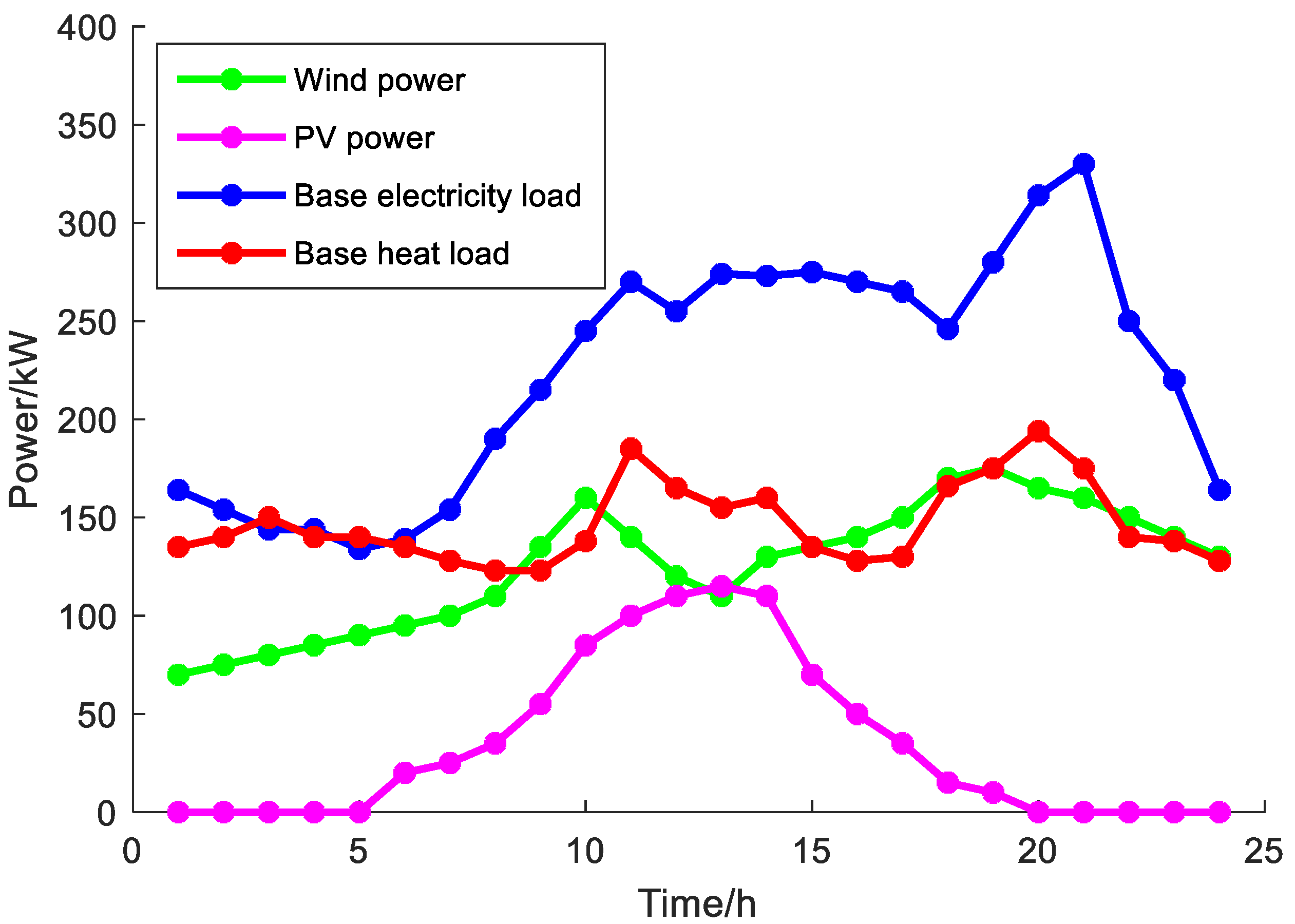
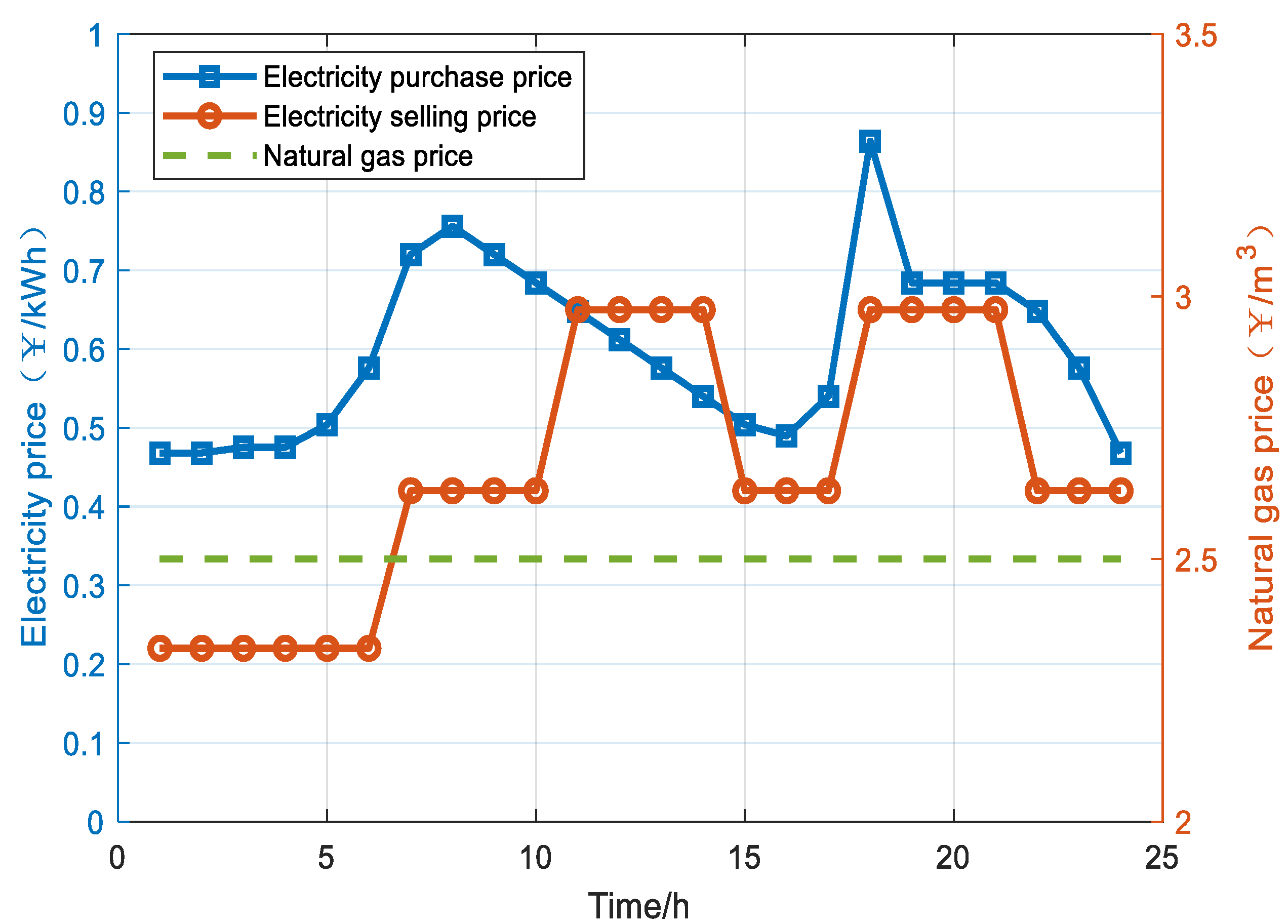
4.1. Parameter Settings

Case studies are presented in this section to verify the low carbon and economy of the proposed dispatch model considering flexible load optimization. The scheduling step is 1 h, and the scheduling cycle is 24 h. The main equipment parameters are shown in

Table 1. Equipment parameters for the integrated energy system.

Equipment	Parameter	Value
GB	${\eta }^{gb}$ $H_{\min }^{gb}$/kW $H_{\max }^{gb}$/kW	0.35 0 150
GT	${\eta }^{gte}$ ${\eta }^{gtl}$ $P_{\min }^{gt}$/kW $P_{\max }^{gt}$/kW $\Delta P_{\max }^{gt,down}$/kW $\Delta P_{\max }^{gt,up}$/kW	0.35 0.10 0 80 15 15
WHB	${\eta }^{wab}$ $H_{\min }^{wab}$/kW $H_{\max }^{wab}$/kW	0.65 0 120
Wind Power Generation System	$C_{wp}$/(CNY/kWh) $C_{wpc}$/(CNY/kWh)	0.50 0.20
PV Power Generation System	$C_{pv}$/(CNY/kWh) $C_{pvc}$/(CNY/kWh)	0.62 0.30
Electricity Energy Storage System	${\eta }^{cha}$ ${\eta }^{dis}$ $c_{ess}$ $P_{\min }^{cha}$/kW $P_{\max }^{cha}$/kW $P_{\min }^{dis}$/kW $P_{\max }^{dis}$/kW $SO{C}_{\min }^e$ $SO{C}_{\max }^e$	0.95 0.95 0.4 30 40 30 40 0.3 1
Heat Energy Storage System	${\mu }^{cha}$ ${\mu }^{dis}$ $h^{loss}$ $c_{hst}$ $H_{\min }^{cha}$/kW $H_{\max }^{cha}$/kW $H_{\min }^{dis}$/kW $H_{\max }^{dis}$/kW $E_{\min }^{hst}$/kWh $E_{\max }^{hst}$/kWh	0.95 0.95 0.001 0.45 20 30 20 30 40 160
Main Power Grid	$P_{\max }^{grid}$/kW	180

. The predicted base electricity load power, base heat load power, and generation of wind and PV power are shown in Figure 3. Time-of-use electricity prices and the natural gas price are shown in Figure 4. Parameters of all types of flexible load are shown in

Table 2. Parameters of shiftable electricity and heat loads.

Load Type	Original Operating Time	Original Load Power	Acceptable Operating Time	Unit Energy Compensation Cost
Shiftable electricity load 1	12:00~13:00	25,24	2:00~10:00	0.2
Shiftable electricity load 2	18:00~20:00	24,25,26	7:00~10:00	0.2
Shiftable heat load	19:00~20:00	15,16	5:00~10:00	0.1

,

Table 3. Parameters of transferable electricity and heat loads.

Load Type	Original Operating Time	Original Load Power	Acceptable Operating Time	Lower and Upper Power Limits	Unit Energy Compensation Cost
Transferable electricity load	12:00~14:00	25,25,25	3:00~10:00	8~26.7	0.3
Transferable heat load	12:00~13:00	20,20	5:00~10:00	8~26.7	0.2

and

Table 4. Parameters of reducible electricity and heat loads.

Load Type	Maximum Allowable Reduction Percentage	Unit Energy Compensation Cost
Reducible electricity load	0.8	0.4
Reducible heat load	0.8	0.2

. The compensation cost coefficients for flexible loads are set to the same value across all time periods.

To verify the proposed low-carbon economic dispatch model and analyze IES scheduling under different scenarios, this paper establishes three typical case studies for numerical analysis.

Scenario 1 (the proposed model): Integrated dispatch model incorporating both ladder-type carbon trading and flexible load optimization.

Scenario 2: Dispatch model considering only the ladder-type carbon trading mechanism.

Scenario 3: Baseline model without carbon trading and flexible load optimization.

All programs are performed on a PC with Intel Core i5-11400H CPU and 16G RAM. The simulation environment is MATLAB R2019b. GUROBI 10.0.3 is used to solve all the optimization problems.

4.2. Results and Analysis

This section is organized into four subsections. The first subsection focuses on the key parameters of the laddered carbon trading mechanism and evaluates their impacts on system costs and carbon emissions through sensitivity analysis. The second subsection presents the optimized scheduling results and the impact of different types of flexible loads on system performance under Scenario 1, where both flexible load optimization and carbon trading mechanism are implemented. Section 3 compares the system performance under different scenarios, and Section 4 discusses the impact of hybrid energy storage system and capacity configuration on system performance.

4.2.1. Sensitivity Analysis of Carbon Trading Parameters

The cost function of the ladder-type carbon trading mechanism includes three key parameters: the carbon trading base price (denoted as n), the price growth rate (m), and the interval length (x). In our simulation experiments, the values of these three parameters are set as follows: n = 250 CNY/t, m = 10%, and x = 0.35 t. They were determined through simulation-based sensitivity analysis. This approach is consistent with many related studies, where the parameters are tuned based on the specific system conditions to achieve a reasonable balance between cost and emission reduction. The simulation results are as follows:

• Impact of Carbon Trading Base Price (n)

As shown in Figure 5, when price growth rate m and interval length x are fixed at 10% and 0.35 t, respectively, an increase in the carbon trading base price leads to a decrease in carbon emissions, but the overall cost of carbon trading rises, and therefore, the total cost of the system increases. When the base price exceeds 280 CNY/t, the decrease in carbon emissions becomes very small, which indicates that the system has reached a relatively stable low-carbon operation state. Therefore, for this test system, the optimal value for this parameter should be maintained below 280 CNY/t.

2.

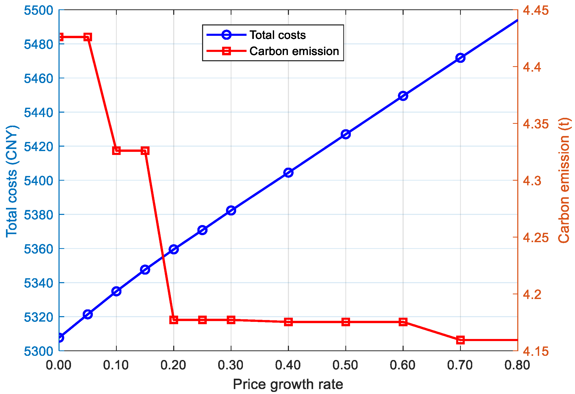
Impact of Price Growth Rate (m)

In Figure 6, with carbon trading base price n = 250 CNY/t and interval length x = 0.35 t, it can be observed that an increase in the price growth rate results in higher carbon trading costs, which, in turn, drives a reduction in carbon emissions. When the growth rate ranges between 10% and 15%, the emission levels begin to stabilize. Further increases beyond 15% lead to additional emission reductions but result in higher total system expenditures. When the price growth rate exceeds 20%, the carbon emissions are no longer further reduced despite continued rate increases, while system operating costs keep rising. Therefore, for this test system, the optimal value for this parameter should be maintained below 20%.

3.

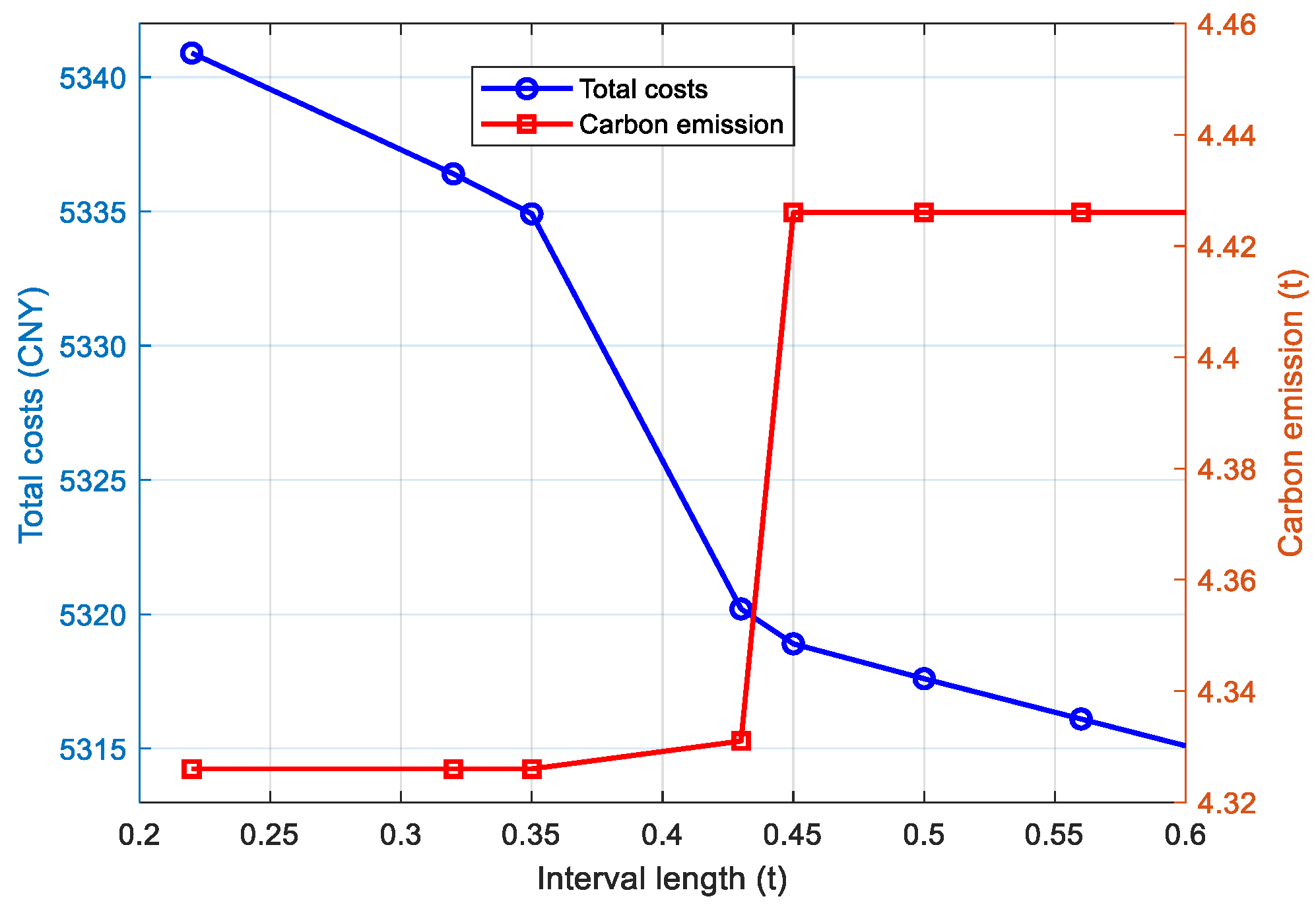
Impact of Interval Length (x):

The interval length (x) defines the threshold of the amount of carbon emissions before entering the next price tier. As can be seen in Figure 7, as the interval length increases, the more carbon emissions the system has, the lower the total cost. This is because, as the interval length increases, fewer tier transitions occur, most of the carbon trading takes place at the carbon trading base price or the first few tiers, and the price is lower, which makes the price signal weaker and leads to more carbon emissions. As shown in Figure 7, for the test system, carbon emissions increase significantly when the interval length is greater than 0.43 t. Therefore, the optimal value for this parameter should be kept below 0.43 t.

These results demonstrate the significant impact of ladder-type carbon trading parameters on the economic and environmental performance of the integrated energy system. Based on the simulation results, we selected the values n = 250 CNY/t, m = 10%, and x = 0.35 t in all case studies.

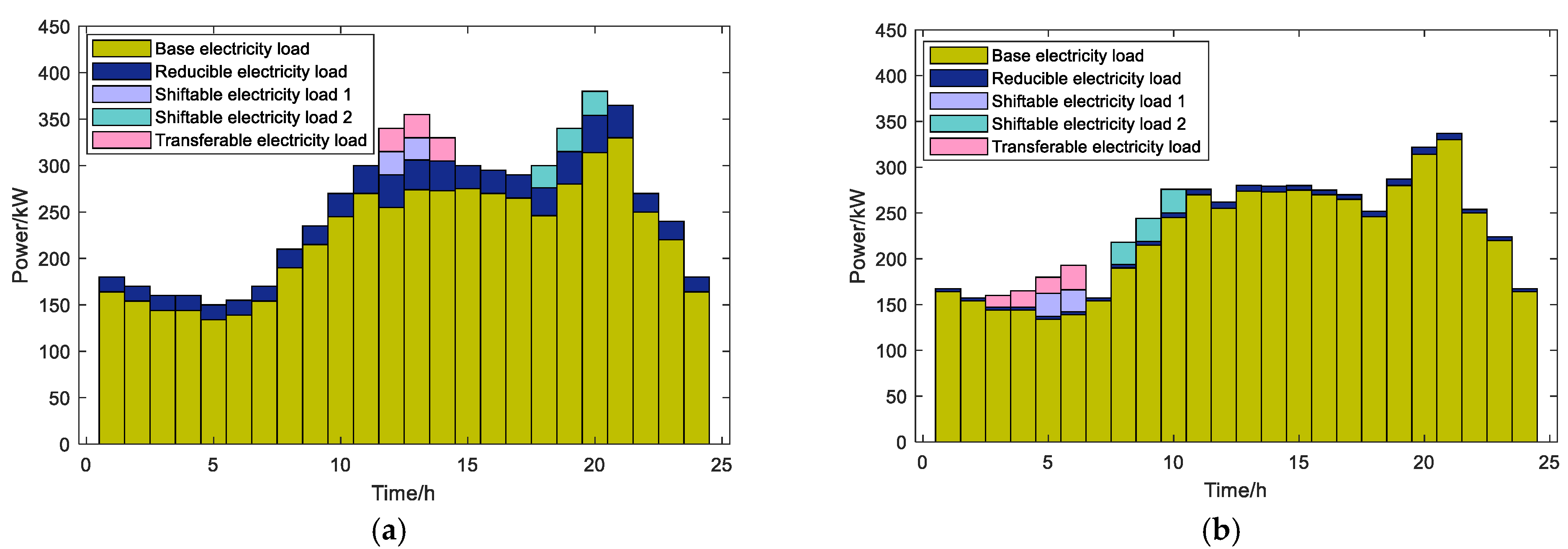
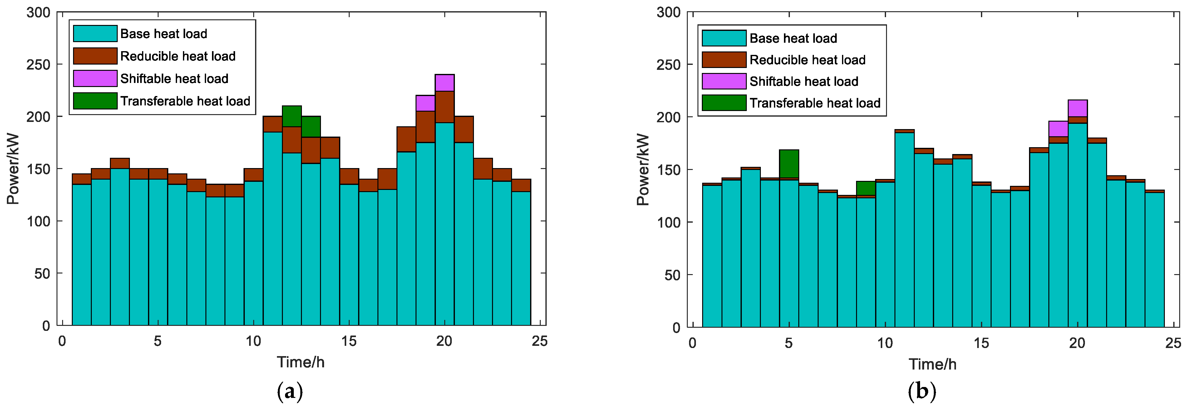
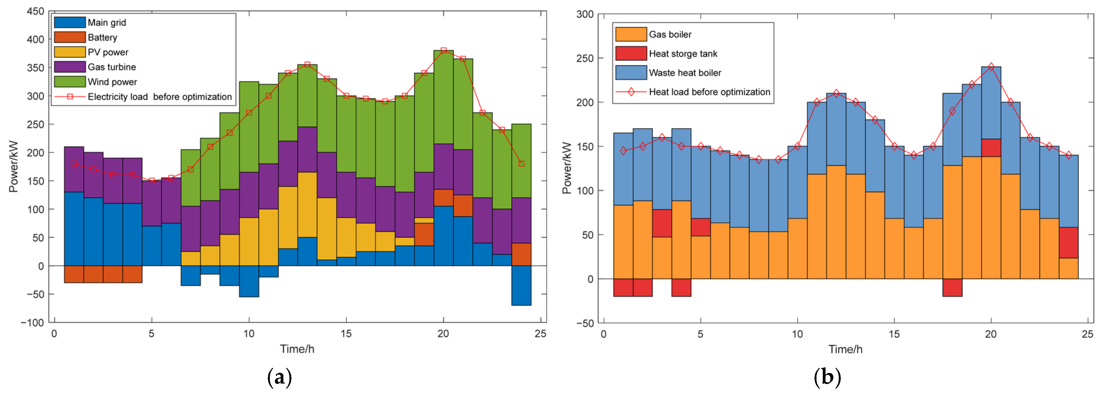
4.2.2. Optimal Scheduling Results Under Scenario 1

The optimal scheduling results of electricity and heat in Scenario 1 are shown in Figure 8, Figure 9 and Figure 10. Comparing Figure 8a,b, it can be seen that for flexible electrical loads, shiftable load 1 is shifted from 12:00–13:00 to 5:00–6:00. Shiftable load 2 is shifted from 18:00–20:00 to 8:00–10:00. Transferable load is rescheduled from 12:00–14:00 to 3:00–6:00. Reducible load is curtailed to varying degrees, with higher reductions during peak periods. For flexible heat loads, as shown in Figure 9, the shiftable thermal load remains unchanged. The transferable thermal load is rescheduled from 12:00–13:00 to 5:00 and 9:00. The reducible thermal load is curtailed more significantly during peak demand. These results validate that the proposed flexible load optimization model effectively coordinates different load types (shiftable, transferable, and reducible) to achieve the desired system performance objectives while maintaining operational constraints. The flexible loads are shifted to specific time periods mainly due to lower electricity prices during those hours, which helps reduce overall operating costs. This price-driven load-shifting strategy effectively utilizes time-of-use pricing to achieve economic benefits while ensuring system reliability.

Figure 10 demonstrates the electricity and heat power optimal dispatch of Scenario 1. From Figure 10a, it can be observed that the electrical load is primarily met by renewable energy and gas turbine output, with a small amount of supplementary power purchased from the grid. As shown in Figure 3, during the 8:00–15:00 period, when wind and solar resources are abundant, excess electricity is sold back to the grid after meeting local demand. The battery storage system charges during low-load periods and discharges during peak-load periods, which not only reduces system operating costs but also alleviates power supply pressure during peak hours. A comparison of the electrical load curves before and after optimization reveals that after flexible load scheduling, electricity consumption increases during the 3:00–10:00 period and decreases during the 10:00–21:00 period. This demonstrates that flexible load optimization effectively flattens the load curve by “peak shaving and valley filling,” reducing peak-valley differences and easing supply pressure during high-demand periods. Additionally, optimized load scheduling facilitates higher utilization of renewable energy.

From Figure 10a,b, it can be seen that the optimization minimizes power purchases from the grid while keeping the gas turbine at full output. Consequently, waste heat recovery is prioritized for heating, supplemented by gas boilers and thermal storage. A comparison of the heat load curves before and after optimization shows that flexible heat load scheduling similarly achieves peak shaving and valley filling, mitigating heating pressure during peak periods.

To further investigate the individual impact of each flexible load type, we conducted three additional simulation experiments, each activating only one type of flexible load. For consistency and fairness, the total load of each type was equally set: 90 kW for electric loads and 50 kW for thermal loads. Additionally, compensation pricing coefficients were set uniformly (0.2 CNY/kWh) across the experiments.

Figure 11, Figure 12, Figure 13, Figure 14, Figure 15 and Figure 16 illustrate the load profile changes before and after optimization for each load type. For example, shiftable electric loads moved from peak to off-peak periods (Figure 11), while shiftable heat loads did not shift due to operational limitations (Figure 14). Transferable electric loads were reallocated from 12:00–14:00 to 04:00–08:00, extending across more time slots (Figure 12), and transferable heat loads were shifted from 12:00–13:00 to 09:00–10:00 (Figure 15). Reducible loads were appropriately curtailed, as shown in Figure 13 and Figure 16.

As shown in

Table 5. System performance under independent optimization of shiftable, transferable, and reducible loads.

Scenario 1	Total Costs (CNY)	Carbon Trading Costs (CNY)	Operation Costs (CNY)	Renewable Energy Output (kW)	Carbon Emission (t)	Renewable Energy Curtailment (kW)	Renewable Energy Curtailment Rate (%)
Only shiftable load	5654.65	282.50	5372.15	3765	4.80	85	2.21
Only Transferable load	5670.05	282.50	5387.55	3775	4.80	75	1.95
Only reducible load	5612.65	282.04	5330.61	3755	4.78	95	2.47

, the results reveal that different flexible load types have varying impacts on system optimization. Among them, reducible loads provided the most significant benefits, resulting in the lowest total cost (CNY 5612.65) and lowest carbon emissions (4.78 t). This indicates that reducing peak loads directly eases system stress, thereby improving both economic and environmental performance. Shiftable loads effectively redistributed demand from peak to off-peak periods, improving load balance, although thermal loads were not shifted, limiting overall gains. Transferable loads offered higher scheduling flexibility but led to the highest system cost (CNY 5670.05), possibly due to the increased complexity or less effective coordination in the specific setup in the test system.

In all the above cases, the compensation cost coefficients for flexible loads are assumed to be fixed across all time periods. To better capture market behavior and improve the responsiveness of flexible loads, a time-of-use (TOU)-based compensation mechanism can be introduced. Under this approach, compensation rates are adjusted according to the temporal variations in electricity prices, incentivizing flexible loads to shift away from high-cost periods and align with system-level economic and low-carbon goals. This dynamic pricing strategy allows for a more accurate representation of demand-side flexibility and enhances the overall efficiency of integrated energy system operations. Future work may further explore the integration of real-time electricity price signals and seasonal carbon price variations into the compensation framework to improve its adaptability and realism.

4.2.3. Comparative Analysis Across Scenarios

Figure 17 and Figure 18 present the optimal power dispatch results for electricity and heat in Scenarios 2 and 3, respectively, providing comparative benchmarks to evaluate the performance enhancements achieved in Scenario 1. The electrical power dispatch in Figure 17a demonstrates Scenario 2’s operational pattern without flexible load optimization, while Figure 18 illustrates Scenario 3’s baseline electricity and heat power dispatch that neither incorporates carbon trading mechanisms nor flexible load optimization. These comparative scenarios serve as critical references for assessing the effectiveness of the proposed ladder-type carbon trading system and flexible load coordination implemented in Scenario 1, particularly in terms of renewable energy utilization efficiency and emission reduction performance. The side-by-side analysis of these dispatch outcomes enables a quantitative evaluation of how each added mechanism contributes to the system’s overall economic and environmental improvements.

Table 6. System performance under different scenarios.

Scenario	Total Costs (CNY)	Carbon Trading Costs (CNY)	Operation Costs (CNY)	Renewable Energy Output (kW)	Carbon Emission (t)	Renewable Energy Curtailment (kW)	Renewable Energy Curtailment Rate (%)
1	5334.91	239.88	5095.03	3850.00	4.33	0	0.00
2	5665.74	282.49	5383.25	3835.00	4.80	15	0.40
3	5347.86	-	5347.86	3335.00	5.53	515	13.38

presents the costs and carbon emissions in different scenarios.

The comparative analysis of three scenarios reveals significant insights about the system’s performance. Scenario 3 exhibits substantial wind curtailment during off-peak periods, while Scenario 2 demonstrates 14.99% improved renewable utilization with correspondingly lower grid purchases, confirming carbon trading’s effectiveness in optimizing the energy mix. Most notably, Scenario 1 achieves the optimal balance with 5.35% lower operating costs (CNY 5095.03 vs. CNY 5383.25), 15.08% reduced carbon trading costs (CNY 239.88 vs. CNY 282.49), and 9.79% lower emissions (4.33 t vs. 4.80 t) compared to Scenario 2 while maintaining the highest renewable output (3850 kW). The carbon trading mechanism alone (Scenario 2 vs. 3) boosts renewable utilization by 15.00% (3835 kW vs. 3335 kW) and cuts emissions by 13.20% (4.80 t vs. 5.53 t) despite modest cost increases of 0.66–5.94%.

These results demonstrate that the integrated approach of ladder-type carbon pricing and flexible load optimization in Scenario 1 creates synergistic effects, delivering superior economic performance (lowest total cost of CNY 5334.91) alongside environmental benefits (minimal emissions of 4.33 t), establishing an effective pathway for low-carbon economic operation of integrated energy systems.

To further evaluate the effectiveness of the proposed flexible load optimization and the ladder-type carbon trading mechanism, this section compares the actual and predicted renewable energy output across different scenarios. Figure 19, Figure 20 and Figure 21 illustrate the renewable energy utilization under Scenarios 1, 2, and 3, providing insights into the impact of the proposed strategies on reducing renewable energy curtailment and enhancing system performance.

As illustrated in Figure 19, Figure 20 and Figure 21, When flexible load optimization is applied (Scenario 1), curtailment is completely eliminated, demonstrating that demand-side flexibility can effectively absorb surplus renewable generation. Comparing Scenario 3 and Scenario 2, the ladder-type carbon trading mechanism reduces curtailment from 515 kW to 15 kW and the curtailment rate from 13.38% to 0.40%, highlighting its role as an effective price-based incentive that prioritizes renewable energy use and improves resource allocation. These findings confirm that both flexible load optimization and the ladder carbon pricing mechanism contribute significantly to curtailment reduction, thereby enhancing renewable energy utilization and supporting the environmental objectives of the system.

4.2.4. Impact of Hybrid Energy Storage System on System Performance

To assess the role of energy storage systems in improving system performance, in this section, we conducted a comparative simulation analysis based on Scenario 1, with and without the inclusion of HESS. Figure 22 and Figure 23 show electric and thermal power dispatch results in Scenario 1 with and without hybrid energy storage.

Table 7. Comparison of system performance in Scenario 1 with and without hybrid energy storage.

Scenario 1	Total Costs (CNY)	Carbon Trading Costs (CNY)	Operation Costs (CNY)	Renewable Energy Output (kW)	Carbon Emission (t)	Renewable Energy Curtailment (kW)	Renewable Energy Curtailment Rate (%)
With energy storage	5334.91	239.88	5095.03	3850.00	4.33	0	0.00
Without energy storage	5463.25	268.20	5195.05	3770.00	4.65	80	2.08

demonstrates a comparison of system performance in Scenario 1 with and without hybrid energy storage. At the same time, this section also analyzes the impact of varying the capacities of BESS and TES on the economic and environmental outcomes of the IES. By isolating the capacity of one storage type while keeping the other fixed, the results reveal how different configurations affect total system cost, renewable energy utilization, carbon trading expenses, and emissions. In the experiment analyzing the impact of varying BESS capacity, TES capacity is fixed at 160 kWh, while BESS capacity is varied across 120 kWh, 160 kWh, and 200 kWh.

Table 8. System performance under different BESS capacities.

BESS Capacity (kWh)	Total Cost (CNY)	Carbon Trading Cost (CNY)	Renewable Energy Output (kW)	Renewable Energy Curtailment (kW)	Carbon Emissions (t)
120	5368.84	243.71	3834	16	4.36
160	5379.07	242.44	3840	10	4.35
200	5334.91	239.88	3850	0	4.33

shows the dispatch results under different BESS capacities. In the experiment analyzing the impact of varying TES capacity, BESS capacity is fixed at 120 kWh, and TES capacity is varied across 120 kWh, 140 kWh, and 160 kWh.

Table 9. System performance under different TES capacities.

TES Capacity (kWh)	Total Cost (CNY)	Carbon Trading Cost (CNY)	Renewable Energy Output (kW)	Renewable Energy Curtailment (kW)	Carbon Emissions (t)
120	5420.53	248.15	3827	23	4.42
140	5394.67	245.93	3831	19	4.38
160	5368.84	243.71	3834	16	4.36

shows dispatch results under different TES capacities.

As shown in Table 7, In terms of economic performance, the total system cost decreased from CNY 5463.25 without HESS to CNY 5334.91 with HESS, and the operation cost dropped from CNY 5195.05 to CNY 5095.03. For environmental performance, carbon emissions were reduced from 4.65 t to 4.33 t, and carbon trading costs also declined. Regarding renewable energy integration, the renewable curtailment was significantly reduced from 80 kW with a curtailment rate of 2.08% to 0 kW with a curtailment rate of 0.00%. At the same time, the total renewable energy output increased from 3770 kW to 3850 kW, indicating that the hybrid energy storage system effectively absorbs surplus renewable generation that would otherwise be curtailed. These improvements result from the enhanced scheduling flexibility brought by HESS. On the electricity side, as shown in Figure 22, BESS charges during low-price or off-peak periods (1:00–6:00), thereby increasing wind power utilization, and discharges during peak demand periods (19:00–21:00), reducing dependence on the power grid. On the thermal side, TES stores surplus heat generated from gas turbines and waste heat boilers and releases it when needed, greatly enhancing the responsiveness and efficiency of the thermal supply.

As shown in Table 8, increasing the BESS capacity has a significant impact on system performance. As the BESS capacity increases from 120 kWh to 200 kWh, the total system cost gradually decreases. Meanwhile, renewable energy curtailment is significantly reduced as BESS capacity increases. In particular, the curtailment drops to zero at 200 kWh, demonstrating that the storage system can fully absorb available renewable energy and thus enhance its utilization efficiency. In addition, both carbon emissions and carbon trading costs show a declining trend, reflecting the positive contribution of BESS to low-carbon system operation. These results indicate that a reasonable increase in BESS capacity can not only improve economic efficiency but also enhance renewable energy integration and reduce emissions, yielding substantial overall benefits.

As shown in Table 9, as the TES capacity increases from 120 kWh to 160 kWh, the total system cost gradually decreases from CNY 5420.53 to CNY 5368.84, and carbon trading costs also show a consistent decline. Meanwhile, renewable energy curtailment slightly decreases, and the corresponding carbon emissions are marginally reduced. These findings indicate that increasing thermal storage capacity can contribute to better cost-effectiveness and improved renewable energy utilization, albeit with limited impact on carbon emissions.

5. Conclusions

This study proposed and validated a ladder-type carbon trading-based low-carbon economic dispatch model for integrated energy systems with flexible load and hybrid energy storage optimization. Three scenarios were simulated to evaluate the impact of carbon trading and flexible load optimization. The ladder-type carbon trading mechanism improves environmental performance by increasing renewable energy utilization and reducing emissions but also raises system costs. Flexible load optimization helps reduce these costs by shifting consumption to periods with lower prices and higher renewable availability, enhancing both economic and environmental outcomes. By enabling flexible charging and discharging, a hybrid energy storage system enhances both electric and thermal scheduling, absorbs surplus renewable energy, and reduces reliance on the grid, contributing to a more efficient and low-carbon operation. The interaction between carbon pricing, demand-side management, and energy storage creates valuable synergies for achieving low-carbon and economic operation of IESs.

However, the current study has certain limitations. The model assumes perfect forecasting of renewable generation and load demand, which may not hold in practical implementations. Additionally, the compensation mechanisms for flexible loads require careful calibration in real-world applications. Future work should address these limitations by incorporating uncertainty quantification and exploring more sophisticated demand response strategies.

References

1. Xu, J.; Chen, Z.; Hao, T.; Zhu, S.; Tang, Y.; Liu, H. Optimal intraday rolling operation strategy of integrated energy system with multi-storage. In Proceedings of the 2018 2nd IEEE Conference on Energy Internet and Energy System Integration (EI2), Beijing, China, 20–22 October 2018; pp. 1–5. [Google Scholar]
2. Li, X.; Wang, W.; Wang, H. Hybrid time-scale energy optimal scheduling strategy for integrated energy system with bilateral interaction with supply and demand. Appl. Energy 2021, 285, 116458. [Google Scholar] [CrossRef]
3. Wang, W.; Huang, S.; Zhang, G.; Liu, J.; Chen, Z. Optimal operation of an integrated electricity-heat energy system considering flexible resources dispatch for renewable integration. J. Mod. Power Syst. Clean Energy 2021, 9, 699–710. [Google Scholar] [CrossRef]
4. Chen, W.; Chen, H.; Chen, J.; Chen, S.; Lin, X.; Li, Y. A Low-Carbon Economic Scheduling Model of Integrated Energy System Considering Ladder-Type Carbon Trading. In Proceedings of the 2022 IEEE 6th Conference on Energy Internet and Energy System Integration (EI2), Chengdu, China, 11–13 November 2022; pp. 2548–2551. [Google Scholar]
5. Chen, J.; Ning, K.; Zhang, Q.; Xu, Q.; Chen, W.; Yu, X. Low-carbon optimization operation of integrated energy system considering ladder-type carbon trading and carbon capture. In Proceedings of the 2022 7th Asia Conference on Power and Electrical Engineering (ACPEE), Hangzhou, China, 15–17 April 2022; pp. 1916–1921. [Google Scholar]
6. Zhang, G.; Liang, J.; Li, F.; Xie, C.; Han, L.; Zhang, Y. Low-carbon scheduling model of electricity-gas-heat integrated energy system considering ladder-type carbon trading mechanism, vehicles charging, and multimode utilization of hydrogen. IEEE Access 2024, 12, 132926–132938. [Google Scholar] [CrossRef]
7. Fan, Y.; Chen, Y.; Cui, M. Electric-Hydrogen Integrated Energy System Optimization Considering Ladder-Type Carbon Trading Mechanism and User-Side Flexible Load. In Proceedings of the 2023 IEEE 6th International Electrical and Energy Conference (CIEEC), Hefei, China, 12–14 May 2023; pp. 1780–1784. [Google Scholar]
8. Zhou, W.; Sun, Y.; Wang, J.; He, Y.; Wu, P.; Chen, L. Robust Optimal Dispatch of Park-level Integrated Energy System Considering Ladder-type Carbon Trading Mechanism. In Proceedings of the 2022 Power System and Green Energy Conference (PSGEC), Shanghai, China, 25–27 August 2022; pp. 38–43. [Google Scholar]
9. Liu, Y.; Li, X.; Liu, Y. A low-carbon and economic dispatch strategy for a multi-microgrid based on a meteorological classification to handle the uncertainty of wind power. Sensors 2023, 23, 5350. [Google Scholar] [CrossRef] [PubMed]
10. Li, C.; Yan, Z.; Yao, Y.; Deng, Y.; Shao, C.; Zhang, Q. Coordinated low-carbon dispatching on source-demand side for integrated electricity-gas system based on integrated demand response exchange. IEEE Trans. Power Syst. 2023, 39, 1287–1303. [Google Scholar] [CrossRef]
11. Li, Q.; He, M.; Tang, X.; Lee, W.-J.; Zhang, Z. Capacity configuration in integrated energy production unit considering ladder-type carbon trading under CCER quota. IEEE Trans. Ind. Appl. 2024, 61, 884–894. [Google Scholar] [CrossRef]
12. Liu, S.; Ma, H.; Huang, C.; Mi, J.; Din, S.; Wang, J. Demand response-based operation optimization of a typical industrial and agricultural IES. In Proceedings of the 2023 IEEE 7th Conference on Energy Internet and Energy System Integration (EI2), Hangzhou, China, 15–18 December 2023; pp. 1065–1070. [Google Scholar]
13. Ma, L.; Han, N.; Chen, S.; Gao, T. A study of day-ahead scheduling strategy of demand response for resident flexible load in smart grid. In Proceedings of the 2020 Management Science Informatization and Economic Innovation Development Conference (MSIEID), Guangzhou, China, 18–20 December 2020; pp. 197–200. [Google Scholar]
14. Tu, J.; Zhou, M.; Cui, H.; Li, F. An equivalent aggregated model of large-scale flexible loads for load scheduling. IEEE Access 2019, 7, 143431–143444. [Google Scholar] [CrossRef]
15. Wang, J.; Liu, J.; Zheng, Y.; Kong, X. Optimal Dispatch of Park-level Integrated Energy System with Flexible Loads and Equipment Variable Operating Conditions. In Proceedings of the 2024 IEEE 2nd International Conference on Power Science and Technology (ICPST), Dali, China, 9–11 May 2024; pp. 1735–1740. [Google Scholar]
16. Wen, Y.; Luo, Y.; Dong, X.; Xie, X. Thermal and electrical demand response based on robust optimization. Electr. Power Syst. Res. 2023, 225, 109883. [Google Scholar] [CrossRef]
17. Wu, M.; Yan, R.; Zhang, J.; Fan, J.; Wang, J.; Bai, Z.; He, Y.; Cao, G.; Hu, K. An enhanced stochastic optimization for more flexibility on integrated energy system with flexible loads and a high penetration level of renewables. Renew. Energy 2024, 227, 120502. [Google Scholar] [CrossRef]
18. Liu, C.; Wang, C.; Yao, W.; Liu, C. Distributed Low-carbon Economic Dispatching for Multiple Park-level Integrated Energy Systems Based on Improved Shapley Value. IEEE Trans. Ind. Appl. 2024, 60, 8088–8102. [Google Scholar] [CrossRef]
19. Zhang, Y.; Sun, P.; Ji, X.; Yang, M.; Ye, P. Low-Carbon Economic Dispatch of Integrated Energy Systems Considering Full-Process Carbon Emission Tracking and Low Carbon Demand Response. IEEE Trans. Netw. Sci. Eng. 2024, 11, 5417–5430. [Google Scholar] [CrossRef]
20. Zhao, H.; Zhang, C.; Zhao, Y.; Wang, X. Low-carbon economic dispatching of multi-energy virtual power plant with carbon capture unit considering uncertainty and carbon market. Energies 2022, 15, 7225. [Google Scholar] [CrossRef]
21. Cui, Y.; Zheng, J.; Wu, W.; Xu, K.; Ji, D.; Di, T. Framework and Outlooks of Multi-Source–Grid–Load Coordinated Low-Carbon Operational Systems Considering Demand-Side Hierarchical Response. Energies 2024, 17, 6208. [Google Scholar] [CrossRef]
22. Li, J.; Yang, W.; Zhang, A.; Li, Q. Low-Carbon Optimal Operation of Park Integrated Energy System Considering Carbon Trading Mechanism. In Proceedings of the 2023 Panda Forum on Power and Energy (PandaFPE), Chengdu, China, 27–30 April 2023; pp. 1086–1091. [Google Scholar]
23. Hu, J.; Liu, X.; Shahidehpour, M.; Xia, S. Optimal operation of energy hubs with large-scale distributed energy resources for distribution network congestion management. IEEE Trans. Sustain. Energy 2021, 12, 1755–1765. [Google Scholar] [CrossRef]
Figure 1. Framework of the integrated energy system.
Energies 18 03679 g001
Figure 2. Ladder-type carbon trading mechanism.
Energies 18 03679 g002
Figure 3. Forecasted profiles of base electricity load, base heat load, and wind and PV power.
Energies 18 03679 g003
Figure 4. Time-of-use electricity purchase and selling prices and the natural gas price.
Energies 18 03679 g004
Figure 5. Impact of carbon trading base price on system costs and carbon emissions.
Energies 18 03679 g005
Figure 6. Impact of price growth rate on system costs and carbon emissions.
Energies 18 03679 g006
Figure 7. Impact of interval length on system costs and carbon emissions.
Energies 18 03679 g007
Figure 8. Power profiles of various electricity loads before (a) and after (b) optimization in Scenario 1.
Energies 18 03679 g008
Figure 9. Power profiles of various heat loads before (a) and after (b) optimization in Scenario 1.
Energies 18 03679 g009
Figure 10. Optimal dispatch results of electric power (a) and thermal power (b) in Scenario 1.
Energies 18 03679 g010
Figure 11. Power profiles of electricity load before (a) and after (b) shifting for shiftable load.
Energies 18 03679 g011
Figure 12. Power profiles of electricity load before (a) and after (b) transferring for transferable load.
Energies 18 03679 g012
Figure 13. Power profiles of electricity load before (a) and after (b) reduction for reducible load.
Energies 18 03679 g013
Figure 14. Power profiles of heat load before (a) and after (b) shifting for shiftable load.
Energies 18 03679 g014
Figure 15. Power profiles of heat load before (a) and after (b) transferring for transferable load.
Energies 18 03679 g015
Figure 16. Power profiles of heat load before (a) and after (b) reduction for reducible load.
Energies 18 03679 g016
Figure 17. Optimal dispatch results of electric power (a) and thermal power (b) in Scenario 2.
Energies 18 03679 g017
Figure 18. Optimal dispatch results of electric power (a) and thermal power (b) in Scenario 3.
Energies 18 03679 g018
Figure 19. Comparison of predicted and actual wind (a) and PV (b) power output in Scenario 1.
Energies 18 03679 g019
Figure 20. Comparison of predicted and actual wind (a) and PV (b) power output in Scenario 2.
Energies 18 03679 g020
Figure 21. Comparison of predicted and actual wind (a) and PV (b) power output in Scenario 3.
Energies 18 03679 g021
Figure 22. Optimal dispatch results of electric (a) and thermal (b) power in Scenario 1 with hybrid energy storage.
Energies 18 03679 g022
Figure 23. Optimal dispatch results of electric (a) and thermal (b) power in Scenario 1 without hybrid energy storage.
Energies 18 03679 g023