Stability Analysis of Power Systems with High Penetration of State-of-the-Art Inverter Technologies

Abstract

With the increasing level of inverter-based resources (IBRs) in modern power systems, this paper presents a small-signal stability analysis for power systems comprising synchronous generators (SGs) and IBRs. Four types of inverter controls are considered: two grid-following (GFL) controls, with or without grid support functions; droop-based grid-forming (GFM) controls; and virtual oscillator control-based GFM. We also analyze the impact of STATCOM and synchronous condensers on system stability to assess their role in the energy mix transition. With the small-signal dynamic behavior of the major technologies modeled, this paper provides stringent stability assessments using the IEEE 39-bus benchmark system modified to simulate future power systems. The exhaustive test cases allow for (a) assessing the impacts of different types and controls of generation and supplementary grid assets, as well as system inertia and line impedance on grid stability, and (b) elucidating pathways for the stabilization of IBR-dominated power systems. The analysis also indicates that future power systems can be stabilized with only a fraction of the total generation as voltage sources without SGs or significant system inertia if they are well distributed. This study provides insights into future power system operations with a high level of IBRs that can also be used for planning and operation studies.

1. Introduction

In recent years, power grids have seen a significant rise in inverter-based resources (IBRs), driven by the need to enhance grid resiliency and meet the rapidly growing energy demands associated with emerging technologies, such as artificial intelligence data centers [1,2,3,4]. IBRs are expected to gradually replace conventional synchronous generators (SGs) and become the dominant interface for diverse energy resources and storage technologies (e.g., wind turbines, solar photovoltaics, hydrogen fuel cells/electrolyzers, and battery energy storage). Since SGs are the primary source of system inertia, their replacement by IBRs leads to a low-inertia grid. The implications of this transition have been extensively discussed in [1,5,6], emphasizing challenges in modeling, control, and stability analysis of IBR-dominated systems. Motivated by these challenges, this work investigates the small-signal stability of power systems under varying control strategies and levels of IBR penetration.

IBRs can be broadly categorized based on their dynamic characteristics into two types: (a) grid-forming (GFM) and (b) grid-following (GFL) inverters. GFM inverters regulate their terminal voltage magnitude and frequency, enabling them to operate independently of SGs. As such, they are considered essential for stabilizing future power systems with high levels of IBR penetration [5]. Depending on the primary control strategy, GFM inverters can be further classified into several types: (a) droop control [7], (b) virtual oscillator control (VOC) [8,9], (c) virtual synchronous machine [10], and (d) matching control [11]. In contrast, GFL inverters synchronize to the grid by tracking the terminal voltage using a phase-locked loop (PLL), and they control output power accordingly [12]. As a result, GFL inverters generally require a stiff voltage reference to maintain stable operation, which raises stability concerns in systems with high penetration of IBRs relying on GFL control. Nevertheless, GFL inverters can provide grid-support functions through supplementary controls, such as frequency–active power and voltage–reactive power droop mechanisms, which will be discussed later. Additionally, other power electronics-based grid-support assets, such as static synchronous compensators (STATCOMs), can be employed for voltage regulation and reactive power support.

System-level stability in power systems integrated with IBRs has been shown to depend heavily on the control strategies employed in the IBRs. In [13], the authors examined small-signal stability across varying penetration levels of droop-controlled GFM and GFL inverters using several benchmark systems. A more targeted analysis of SG and IBR interactions, specifically for droop-controlled GFM and conventional GFL inverters, is presented in [14]. However, these studies do not consider alternative GFM control strategies or the role of grid-supporting devices such as STATCOMs and synchronous condensers (SCs). Furthermore, the test systems used in [14,15] involved only a few SGs and inverters, which limits their ability to capture the dynamic behaviors of large-scale bulk power systems with multiple interacting sources. The stability of VOC has been investigated in [16,17], focusing on scenarios with either islanded inverters or simplified setups involving one inverter and one SG. A comparative study between VOC and droop-controlled GFMs is provided in [18], yet none of these efforts include a comprehensive stability assessment of VOC in a realistic bulk system comprising diverse IBR technologies. In [19], the stability implications of both GFM and GFL inverters have been explored; however, the analysis does not extend to a complex power system containing multiple IBRs and SGs operating in concert.

As IBRs gradually displace conventional SGs, existing SGs can be repurposed as SCs to continue contributing to system stability through reactive power support, voltage regulation, and inertia retention. While the potential of SCs has drawn increasing attention [20,21], their role in stabilizing systems under different levels of IBR penetration remains insufficiently understood. Notably, some functions provided by SCs, such as voltage and reactive power support, can also be delivered by power electronic devices like STATCOMs or GFL inverters. The stabilizing effect of STATCOMs on small-signal dynamics has been demonstrated for the IEEE 39-bus system in [22], but the study only considered systems composed entirely of SGs. The impact of STATCOMs on system stability in environments with both SGs and IBRs has yet to be comprehensively addressed. Similarly, while ref. [23] compares SCs and STATCOMs from an inertia standpoint, a broader comparison of these technologies within a heterogeneous system containing multiple IBRs and SGs is still lacking.

In addition, transmission line characteristics also play a significant role in determining the stability of IBR-rich systems. For example, ref. [24] reported that increasing line admittance may destabilize power systems with dispatchable VOC-based GFMs. Similarly, refs. [25,26] established an inverse relationship between line impedance and grid strength. Nevertheless, these works do not examine the influence of line impedance across different levels of IBR penetration or control strategies, leaving another gap in the current understanding.

To address these limitations, this paper presents a comprehensive extension of the prior work documented in [27]. Since small-signal analysis enables stability assessment through a simplified linear model, it allows for direct evaluation of the stability of steady-state operating points. This forms a fundamental part of power system analysis, as ensuring the stability of these points is a prerequisite for exploring broader system dynamics and operational behaviors. Therefore, the focus of this work is on evaluating and interpreting the small-signal stability of a bulk power system in which SGs are progressively replaced by IBRs. The analysis was conducted using the widely adopted IEEE 39-bus benchmark system, which was chosen for its representative architecture and topology. A diverse set of grid assets was modeled to reflect realistic scenarios, including SGs, various types of IBRs, such as GFM inverters with droop and VOC, and GFL inverters with and without grid-support functionalities, as well as grid-supporting devices, including STATCOMs and SCs.

While power system stability is often highly case-specific, this study emphasizes the general characteristics of IBR technologies and their impacts on the small-signal stability of large power systems to provide insights into future power system operations with a high level of IBRs that can be leveraged for planning and operation studies. For detailed case studies on specific systems, readers are referred to [1,28,29]. The stability assessment demonstrates that the maximum stable IBR penetration level is highly sensitive to multiple factors, including control strategies, generator placement (i.e., electrical distance), and specific control parameter settings. To explore potential configurations for future power systems with diverse generation technologies, additional case studies investigate scenarios in which multiple generator types are co-located at each bus. The results highlight the stabilizing effect of strategically distributing a number of voltage-source elements (SGs and GFMs) throughout the network. Lastly, the paper examines how local variations in network impedance, particularly near stability-sensitive buses, influence overall system behavior, using participation factor analysis to identify the most influential components.

The key contributions of this paper are summarized as follows:

• A comprehensive small-signal stability assessment is presented for a bulk power system with mixed SG and IBR penetration, revealing how control strategies, parameter settings, and structural characteristics, including inertia and impedance, affect system stability.
• The study demonstrates the stabilizing role of supplementary grid assets (SCs and STATCOMs) and highlights the benefits of strategically distributing a sufficient number of voltage-source elements (SGs and GFMs) throughout the system to enable high penetration of passive assets, such as GFL IBRs.

The paper is organized as follows. Section 2 provides the dynamic modeling of the generation technologies under study. Section 3 discusses the IEEE 39-bus test system model for analysis and the network modeling to integrate multiple generator dynamics at different buses for exhaustive test cases. Section 4 presents the small-signal stability analysis of the multiple exhaustive test cases developed to pinpoint the stability impact of different technologies and transmission lines, along with a discussion to provide insights into bulk power system stability. Section 5 concludes with final remarks and future work.

2. Dynamical Models

The dynamical models and control strategies of the different types of generators studied in this work are briefly described in this section. For the modeling, all the three-phase voltage and current signals were converted to the synchronous reference frame (dq frame). The fundamental frequency was determined by the rotor frequency for SGs, the PLL output frequency for GFL inverters, and the controller-generated terminal voltage frequency for GFM inverters.

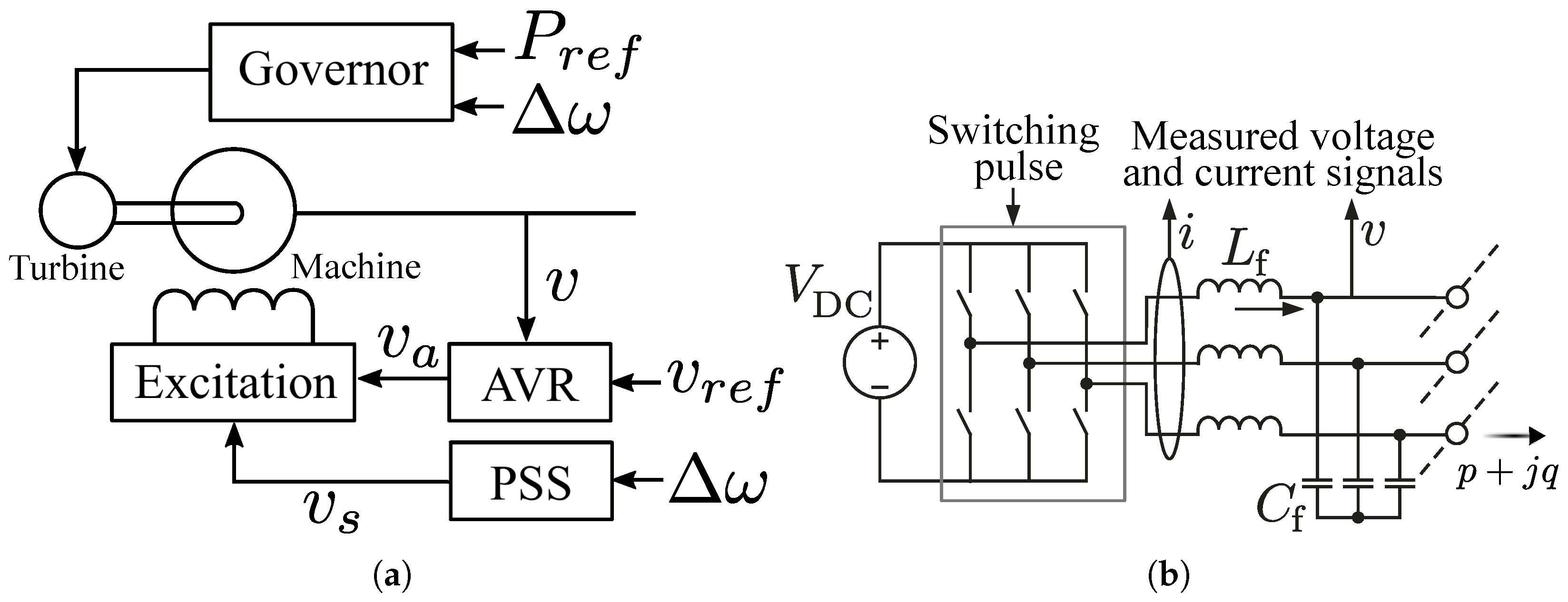
2.1. Synchronous Generators

Synchronous generators are the most common type of power generation that converts mechanical power from a prime power source (e.g., hydro and thermal) into electrical power. It mainly consists of a rotor, stator, rotating turbine, and controllers, as illustrated in Figure 1a. For the small-signal stability analysis, the 4th-order model of the SG is considered (shown in Equations (1)–(4)), where the states are the d- and q-axis voltages behind the transient reactances, the machine angle, and the machine speed. The SGs in this study are equipped with a power system stabilizer (PSS), automatic voltage regulators (AVRs), and governors. A governor model with a single state is used to regulate the output power based on the generator speed deviation from the nominal operating point. Static AVR with four states and $\Delta \omega$ PSS with three states are modeled here to control the terminal voltage and to improve the stability, respectively. The state-space equations are provided in detail in [29,30]. The swing equation, as shown in Equation (2), represents the state equation for the frequency ($\omega$) of the SG, where H is the mechanical inertia of the machine, and $T_m$, $T_e$, and $T_f$ are the mechanical, electrical, and frictional torque, respectively.

$$\begin{array}{cc}\hfill \dot{\delta }& ={\omega }_b(\omega -1)\hfill \end{array}$$

(1)

$$\begin{array}{cc}\hfill 2H\dot{\omega }& =T_m-T_e-T_f\hfill \end{array}$$

(2)

$$\begin{array}{cc}\hfill T_{do}^{\prime }{\dot{E}}_q^{\prime }& =-E_q^{\prime }-(X_d-X_d^{\prime })I_d+E_{fd}\hfill \end{array}$$

(3)

$$\begin{array}{cc}\hfill T_{qo}^{\prime }{\dot{E}}_d^{\prime }& =-E_d^{\prime }+(X_q-X_q^{\prime })I_q\hfill \end{array}$$

(4)

The rotating mass of the SG is the source of the mechanical inertia that decelerates the frequency change under a disturbance by balancing the discrepancy between supply and demand with the energy stored in the rotor. As a result, it helps maintain the frequency stability of the power system after a contingency. Also, SGs regulate the terminal voltage and frequency at the designed value with the AVR and droop. The governor adjusts the output power based on the frequency deviation and droop laws, which helps synchronize the frequency and share the active power demand across generators in the grid.

2.2. Inverter-Based Resources

Voltage-source inverters with output LC filters are adopted for the inverter models, as illustrated in Figure 1b. An averaged inverter model is employed under the assumption that the inner-loop control and switching dynamics are significantly faster than the primary control and grid dynamics, a condition generally valid for most power conversion devices. This allows the analysis to focus on the interactions between the primary controllers and the rest of the system. To simplify the model, the dynamics of the dc-side sources (e.g., battery or photovoltaic array with or without power electronics interface) are omitted. We assume that the dc-link voltages of IBRs are tightly regulated or that the dc sources are designed properly, thus remaining constant, which simplifies the small-signal model. This assumption is justified for the following three reasons. First, most IBRs are equipped with energy storage or appropriate source-side control to mitigate fluctuations in generation, and they are designed with internal controllers that ensure tight regulation and stability. Second, variations in IBR power set points typically originate from dispatch commands, which evolve on much slower timescales than the small-signal dynamics of interest in this study. Therefore, their influence can be neglected in the small-signal model. Third, the dc-link voltage dynamics could contribute to system instability, especially in abnormal operating conditions, but analyzing such effects falls outside the primary scope of this work. This work focuses on system-level small-signal stability, which assumes that each IBR or generator has well-designed control for its prime sources.

The filter capacitor ($C_f$) voltage, v, and the filter inductor ($L_f$) current, i, are measured and used for the converter control. As discussed in Section 1, the IBRs are broadly divided into two categories: (a) GFM—the inverter controls the terminal voltage and frequency, i.e., a controlled voltage source—and (b) GFL—the inverter tracks the terminal voltage using a PLL to supply the reference power to the grid, i.e., a controlled current source. The GFM and GFL inverter controls can be implemented in different ways. In the following, some representative control methods are discussed.

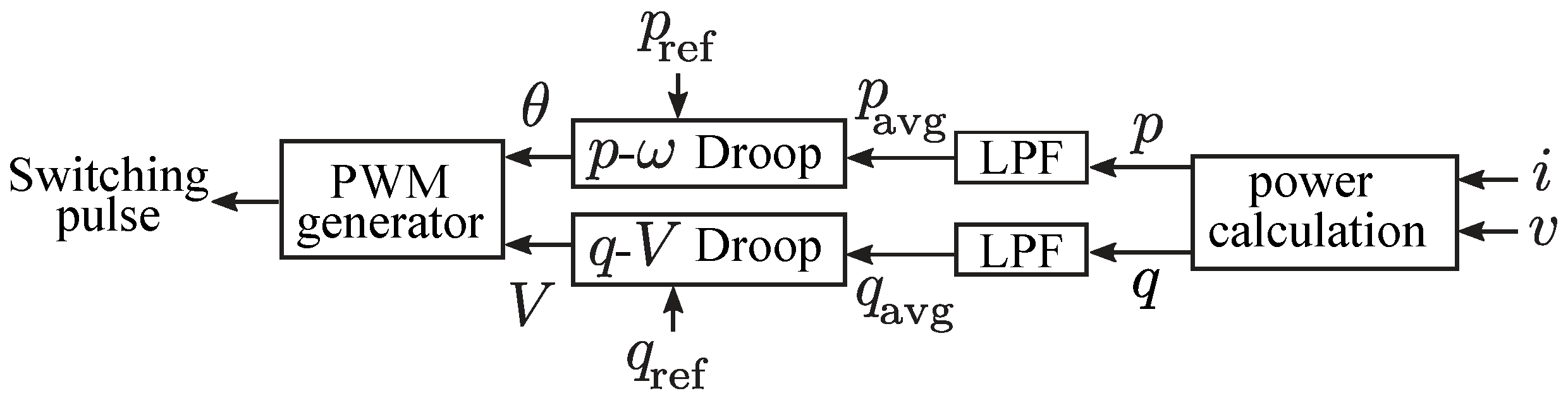
2.2.1. Droop-Controlled Grid-Forming Inverters (Droop-GFM)

The droop control decides the terminal voltage magnitude ($V_c$) and frequency (${\omega }_c$) for this class of GFM inverters and is expressed as [31]

$$\begin{array}{c}\hfill {\displaystyle \frac{d}{dt}}{\theta }_c={\omega }_c={\omega }_{nom}+k_p(p_{ref}-p_{avg}),\end{array}$$

(5a)

$$\begin{array}{c}\hfill V_c=V_{nom}+k_q(q_{ref}-q_{avg}).\end{array}$$

(5b)

Here, as shown in Figure 2, p and q are instantaneous active and reactive power generation from the inverter, respectively. $p_{avg}$ and $q_{avg}$ are low-pass-filtered versions of p and q to limit the effect of high-frequency noise and disturbances, which are processed with the reference values for droop, $p_{ref}$ and $q_{ref}$, respectively. $k_p$ and $k_q$ are droop gains used to determine the amount of frequency and voltage droops.

For the small-signal stability analysis, the filtered active ($p_{avg}$) and reactive powers ($q_{avg}$), the angle of the terminal voltages (${\theta }_c$), and the voltages (v) and currents (i) at the LC filter in the $d-q$ reference frame are the states.

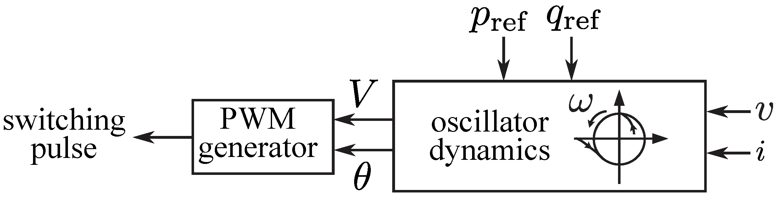
2.2.2. Virtual Oscillator-Controlled Grid-Forming Inverters (VOC-GFM)

The dispatchable VOC-based GFM inverter models are used here, as shown in Figure 3. This time-domain control strategy replicates a nonlinear oscillator behavior by using the measured current as the input. For this small-signal model, the output voltage magnitude and angle are considered states. Also, the voltages and currents of the LC filter in the $d-q$ domain are the other four states in the model. Interested readers are referred to [8] for more details of VOC-GFM.

Both Droop-GFM and VOC-GFM regulate the terminal voltage and frequency, and their steady-state behavior is similar [32]. So, from the small-signal stability perspective, they may exhibit similar results, as shown later in this paper; however, it should be noted that their dynamic responses may differ, which is not in the scope of this study [18].

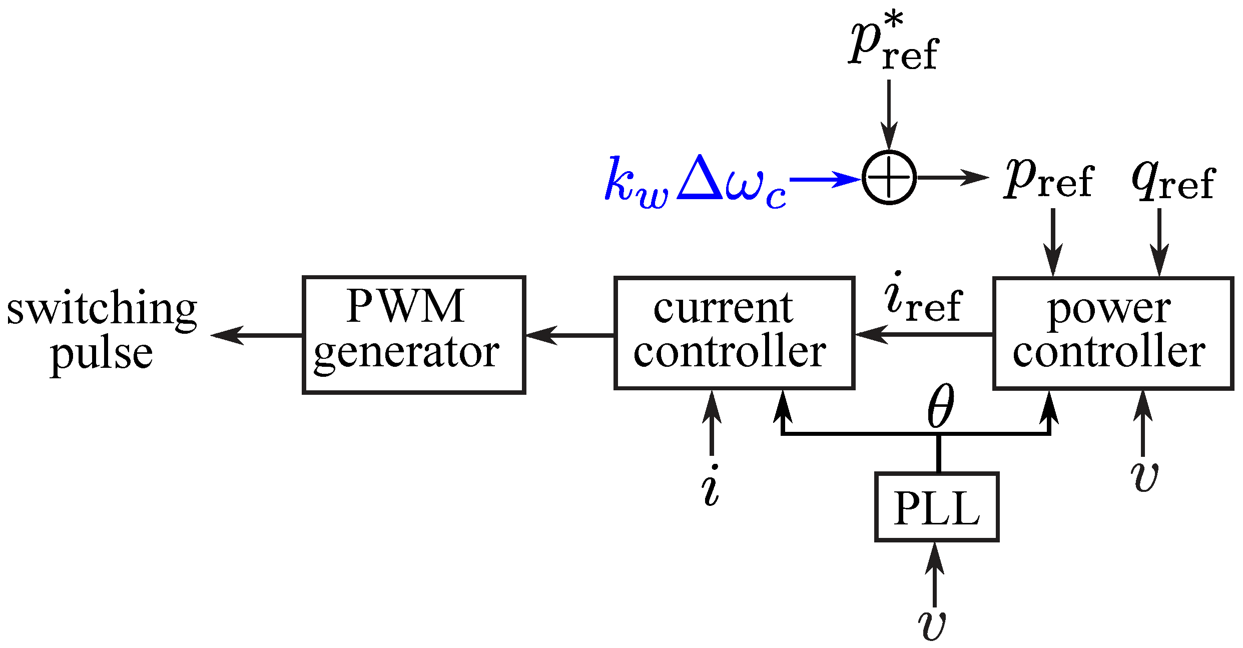
2.2.3. Grid-Following Inverters (GFL)

This study models a GFL inverter that follows the voltage and frequency at the point of common coupling (PCC) with a PLL. The PLL takes the terminal voltage as input and generates the frequency and angle reference ($\theta$) for the power and current controllers, as illustrated in Figure 4. The power controller tracks the active and reactive power references and generates the $d-q$ domain current references, which the current controller further uses. The current controller generates the modulation signals for the pulse width modulation. Figure 4 displays the GFL control diagram with the part in blue applicable for droop control (discussed next). The state-space model for the GFL inverters consists of states for the filtered active and reactive power, four states for the currents and voltages of the LC filter in the $d-q$ domain, and states for the power and current controllers.

This study models a generic PLL with a low-pass filter and a PI controller to provide general insights into its impact on system stability. The PI-controlled PLL can be expressed as as [31]:

$$\dot{\theta }={\omega }_{PLL}={\omega }_{nom}+k_{PLL}^p{\dot{\varphi }}_{PLL}+k_{PLL}^i{\varphi }_{PLL}.$$

(6)

Note that GFL inverters may use a different control structure for a PLL or have a different control mechanism, i.e., no PLL, for grid synchronization [33,34].

For the GFL inverter model with the grid support functions, this study models the active and reactive power references drooped with the frequency and voltage deviation from the nominal values, respectively, which are expressed as [31]:

$$\begin{array}{c}\hfill p_{\mathrm{ref}}=k_{\omega }({\omega }_c^{*}-{\omega }_c)+p_{\mathrm{ref}}^{*},\end{array}$$

(7a)

$$\begin{array}{c}\hfill q_{\mathrm{ref}}=k_v(V^{*}-V)+q_{\mathrm{ref}}^{*},\end{array}$$

(7b)

where, ${\omega }_c^{*}$ and $V^{*}$ are the nominal frequency and voltage values. Also, $k_{\omega }$ and $k_v$ are the droop gains for generating the active and reactive power references, respectively.

Note that for the GFL with droop (GFLD) inverter, the power references are drooped with the frequency and voltage deviations; on the other hand, for the droop-GFM inverter, the terminal voltage and frequency are directly controlled based on the active and reactive power outputs. As a result, compared to the GFM control, the grid support with the GFLD inverter indirectly controls the output frequency and voltage, contributing to the system stability while still relying on the PLL. Figure 4 illustrates the GFLD inverter control with the additional term highlighted in blue, $k_{\omega }\Delta {\omega }_c$, where $\Delta {\omega }_c={\omega }_c^{*}-{\omega }_c$.

2.3. Other Grid-Supporting Assets

2.3.1. Synchronous Condensers

An SC can be used to provide reactive power support to the grid to help regulate the line voltage and maintain the power factor. The SC can be considered a synchronous machine without the prime mover or mechanical load. For the state-space model of an SC, therefore, the SG model is modified by eliminating the state of the mechanical power [29,30]. This makes the frequency state Equation (2) of an SG become

$$\dot{\omega }={\displaystyle \frac{1}{2H}}(-T_e-T_f).$$

(8)

Now, as shown, only the frictional torque is balanced with the electrical torque generated. A small amount of negative active power generation is modeled to replicate the mechanical loss from the machine.

2.3.2. STATCOMs

STATCOMs can be modeled as a voltage-source inverter that can support the grid with reactive power and regulate the PCC voltage. It can be considered as a GFL inverter without an active power supply. For the state-space modeling, the GFL inverter model with a PLL and reactive power control is used in this study [31]. Similar to the GFLD inverter, the reactive power reference is drooped with the voltage deviation from the nominal value as

$$q_{\mathrm{ref}}=k_v(V^{*}-V)+q_{\mathrm{ref}}^{*}.$$

(9)

Here, the active power reference is set to a small value to solve the load flow and justify the converter loss to regulate the inverter dc-link voltage.

Table 1. Overview of power grid generation and support technologies for stability analysis.

Gen. Type	Grid Support Functionality	Notable Features
SG	Provides voltage and frequency regulation based on electro-mechanical coupling and provides rotational inertia.	Has been the foundation for legacy grids. Can stabilize a grid independently and provides support during contingencies in the grid.
GFM	Regulates the voltage and frequency based on the inverter terminal measurements with droop characteristics programmed. No mechanical inertia is present because this is a power electronics inverter-based resource.	Frequency-watt and voltage-VAR droops help multiple generators share loads and collectively maintain the grid. Backward compatible with SGs. Theoretically, small-signal stable at 100% IBR penetration level for a bulk grid.
GFL	Provides constant power/current at the inverter terminal. The terminal voltage and frequency depend on the rest of the grid.	Most popular control method for field-deployed IBRs. Cannot maintain grid stability alone for $100\%$ IBR penetration level.
GFLD	Provides constant power/current with droops on the active and reactive power references based on the frequency and voltage deviation from the nominal values.	Provides better grid support than normal GFL inverters; however, it might not firmly maintain grid stability alone, since there is no explicit control on the terminal voltage and frequency like a GFM inverter. Due to this, cannot ensure stability for a grid with $100\%$ IBR penetration.
SC	Provides only voltage-reactive power regulation and rotational inertia.	Provides grid support with voltage regulation and can contribute to frequency stability, since the mechanical inertia is present.
STATCOM	Provides reactive-power support and voltage regulation. No mechanical inertia is present because this is based on a power electronics inverter.	Can contribute to system stability using adaptive reactive-power provision.

summarizes the power grid generation and support technologies included in this stability analysis study.

3. Description of Test System

The IEEE 39-bus system, also known as the 10-machine New England power system, was considered as the base case for this study. The detailed parameters of the buses, lines, loads, and generators are provided in [35]. As shown in Figure 5, buses 30–39 contain generators. This study investigates the small-signal stability of the 39-bus system in which the eight generators at buses 31–38 (all SGs in the base model for fossil-fueled or nuclear power plants) are replaced entirely or partially by IBRs or IBRs with other grid-supporting assets. The replacement exemplifies future power systems with increased IBR penetrations. The generators at buses 39 and 30 are not replaced, considering that the generator at bus 39 is the equivalent representation of a large number of generators and networks, i.e., the rest of the interconnection. The hydro generator at bus 30 maintains the minimum system inertia.

3.1. Stability Analysis Method

For the stability analysis, the dynamic state equations for the plants and the network line model were used. The dynamic model of the generators and inverters is expressed in the generic form as

$$\dot{x}=f(x,u,z).$$

Here, x defines the states of the machines and inverters, u defines the external control inputs, and z is the interface variable with the algebraic equations. The line data of the 39-bus system were used to build the admittance matrix ($39\times 39$) for the entire grid. Next, the $10\times 10$ admittance matrix for only the buses with power plants was obtained using Kron reduction. This admittance matrix was used to obtain the algebraic equations between x, u, and z as

$$z=g(x,u).$$

Based on the system representation, the dynamic model can be linearized around the operating point, and the eigenvalues are identified for stability assessment. In this study, the entire model of the grid was developed, and it was numerically linearized at the steady-state operating point to construct the state-space matrix. This matrix was further used to obtain the eigenvalues.

3.2. Connecting Multiple Types of Generator at One Bus

In Section 4, we also consider the cases of having multiple types of power generations at one generator bus. For this scenario, the existing total generation from one plant is divided into two or three separate smaller plants (e.g., SG + GFM + GFL at a bus) to retain the same load flow at all buses. For computation, those plants are connected through separate branched sub-buses, which are connected to the original generator bus through transmission lines with negligible impedance.

The modeling approach considered different scenarios where the total generation from the original plant was divided into smaller plants with different fractions. This was to evaluate the impact of the fractional penetrations on the system stability as a potential practical approach to stabilize future grids with GFM assets accounting only for a fraction of the total generation. We scaled the plant parameters based on the plant power rating and the original generation parameters to model the dynamics of generators at different scales. More details are provided in Appendix A.

4. Case Studies and Discussion

Based on the modeling and test system discussed, this section presents case studies followed by a discussion to analyze and provide insights into the bulk power system stability. In the test cases, the synchronous generators in the baseline model of the IEEE 39-bus system were replaced by IBRs with state-of-the-art control inverter technologies or SCs to analyze the impact of the energy mix transition. These cases represent the transformation of legacy grids through the integration of IBRs, and we focus on the small-signal stability of those cases. We discuss notable cases, observations, and interpretations that will help stabilize the IBR-dominated future grids.

4.1. Baseline Case—All Synchronous Generators

The baseline case retains all the plants as SGs, representing the legacy power system without IBRs. The power flow solution in the baseline case is benchmarked with the case in [29], and it is small-signal-stable. Small-signal stability is analyzed by identifying the rightmost eigenvalue throughout the paper.

4.2. One-by-One Replacement of IBRs

In this subsection, generators were replaced by IBRs, plant by plant, to examine the effect of IBR penetration at the plant level. In the test cases, Gen 2–9 were replaced by IBRs with the same power rating as the original plant.

To provide insights into the roles and impact of IBRs on the system stability, this analysis examined the stability of a system with voltage-source generators (either SG or GFM) and current-source generators (GFL). Six sets of stability results are displayed in Figure 6: (a) SG and GFL, (b) SG and GFLD, (c) Droop-GFM and GFL, (d) Droop-GFM and GFLD, (e) VOC-GFM and GFL, and (f) VOC-GFM and GFLD. In each scenario, two types of plants were considered with all possible combinations ($2^8=256$) at Gen 2–9 in the IEEE 39-bus system. Different shades of green and red distinguish the stable and unstable cases, respectively. Here, darker shades represent a higher magnitude of the real part of the rightmost eigenvalue. Therefore, a darker green shade indicates a more stable scenario, and a darker red represents a more unstable case.

4.2.1. Impact of GFL Inverter on Stability

When the existing SGs were replaced one by one with GFL inverters, only a fraction of the modified cases were small-signal-stable, as shown in Figure 6a. The system became unstable with the GFL inverters when a specific SG(s) was replaced with a GFL inverter(s). Notably, the system stability was not directly related to the generation proportion of the IBRs, which will be discussed later. For this system, $46.5\%$ of the total possible cases with SGs and GFL inverters were stable.

4.2.2. Impact of GFL Inverter with Droop Control on Stability

Next, the impact of the grid support functionality integrated with the GFL inverters, i.e., GFLD, is discussed. In the GFLD IBRs, the active power reference was drooped with the frequency deviation, and the reactive power was drooped with voltage deviation (IBR operation with a headroom was assumed). These GFLD inverters improved the system stability compared to the ones with GFL inverters, as shown in Figure 6b. As presented, some cases that were unstable with GFL in Figure 6a became stable when the grid support functionality was added, while stable cases remained unchanged. Almost $60\%$ of the total possible cases were stable when the existing SGs were replaced with GFLDs, illustrating the benefit of the grid support functions of GFL inverters. Note that different control methods can be used to implement GFLD inverters; thus, they can affect the system stability differently.

Observation: Achieving IBR-dominated power systems entirely with only GFL inverters, either GFL or GFLD, is impossible, though GFLD improves the system stability over GFL. Also, at the same level of GFL inverter penetration, the system can be stable or unstable depending on the IBR location; generation asset allocations significantly affect the IBR penetration level reachable.

4.2.3. Impact of GFM Inverters on Stability

Next, all the plants at Gen 2–9 were replaced with IBRs, which is a close representation of the future scenario with $100\%$ IBRs in the power grid. The possibilities of integrating GFM and GFL inverters with different control types were considered at different buses, which are shown in Figure 6c–f. First, with GFMs, either Droop-GFM or VOC-GFM, and GFL inverters, $37.9\%$ of the cases were stable for 256 possibilities, as shown in Figure 6c,e. Next, the GFL inverters were replaced with GFLD inverters, as presented in Figure 6d,f. The grid-supporting controls helped achieve stability for a few unstable cases with the GFL inverters, and as a result, about $39\%$ of the total cases were stable with GFLD and GFM.

Observation: The Droop-GFM and VOC-GFM have a comparable impact on the small-signal stability. Also, GFLD inverters are marginally beneficial for an IBR-dominated power grid in the one-by-one replacement scenarios. Due to the presence of mechanical inertia, SGs could be better than GFM inverters for overall system stability, primarily when generators are located at a distance. More discussions are found in Section 4.5. Also, the overall system’s stability depends not only on the total IBR penetration level but also on the location of the IBRs, which is explored later in detail.

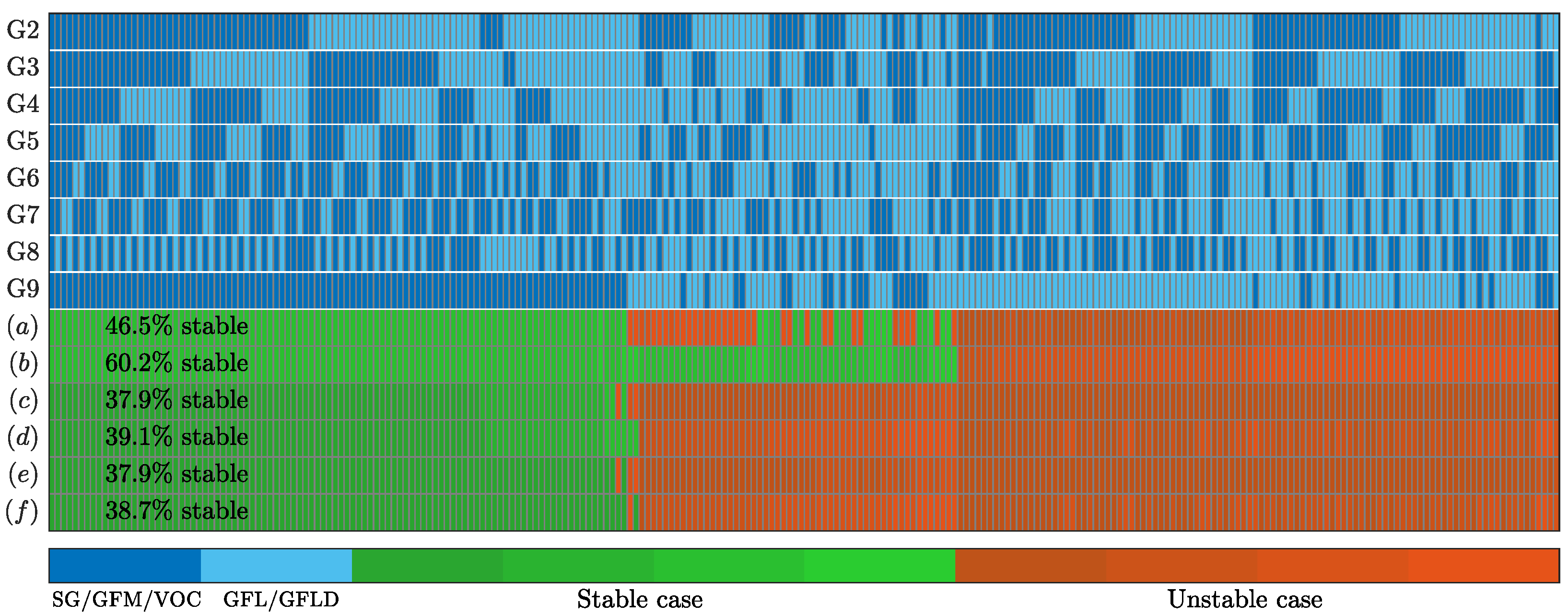
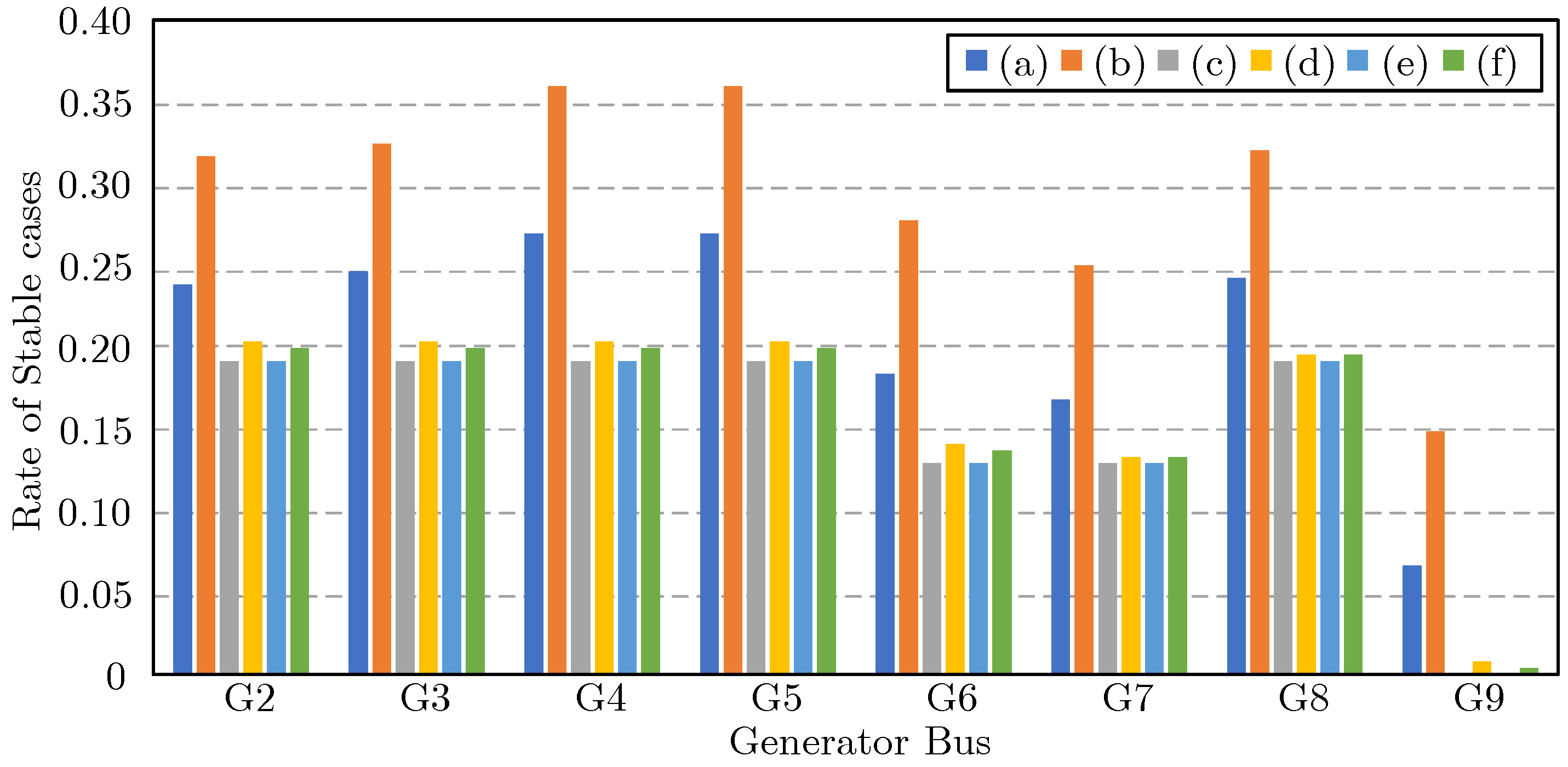
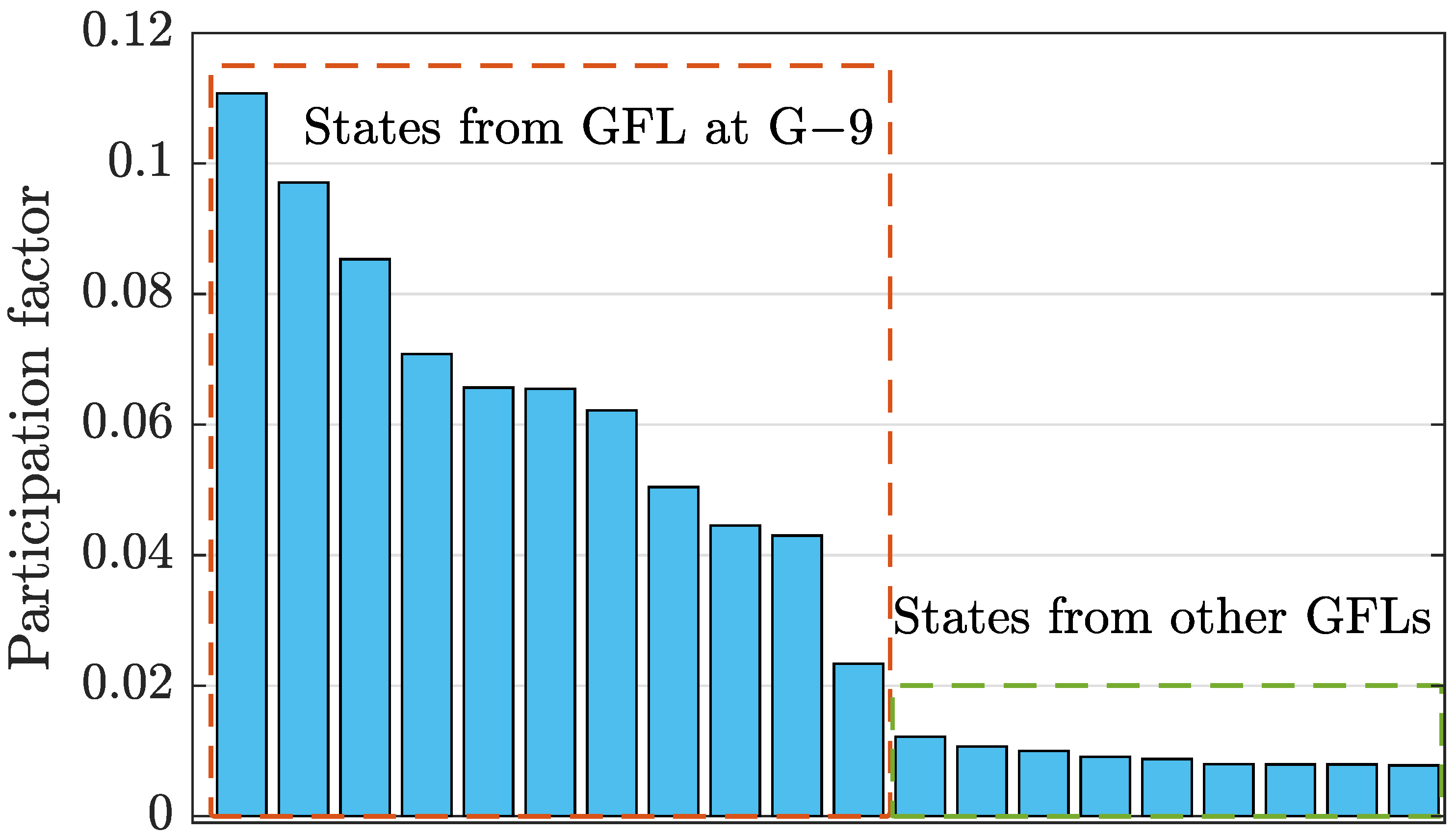
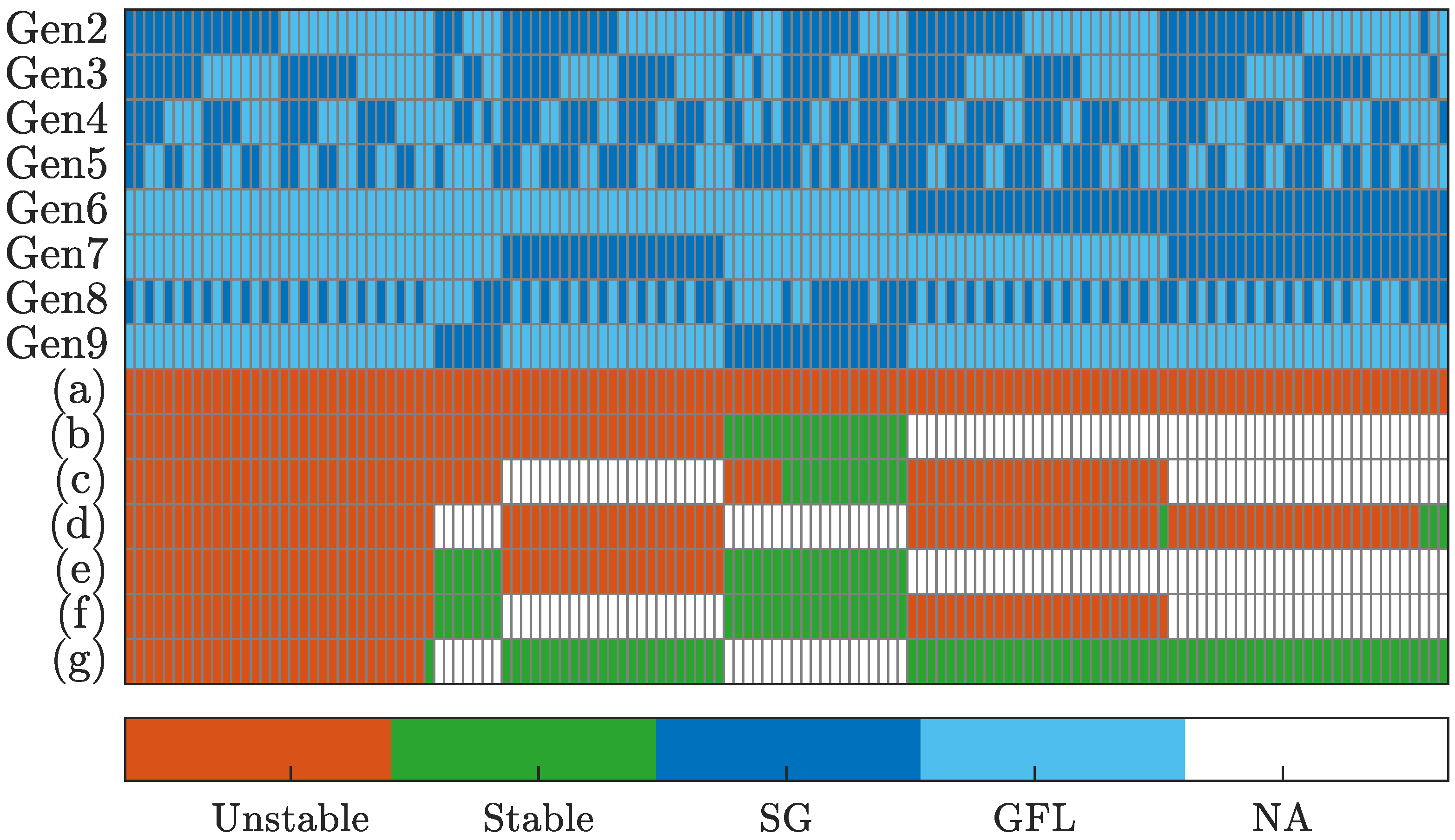
4.3. Identifying the Most Vulnerable Generator Bus in the Presence of IBRs

In the preceding sections, we observed that the system stability relates to the location of the generators. To examine this, the unstable cases were further analyzed. As noticeable in Figure 6, replacing Gen 9 with a GFL IBR caused most of the instability.

The fraction of stable cases when each of Gen 2–9 was replaced with a GFL inverter is illustrated in Figure 7 for all six scenarios discussed in Section 4.2. As shown in Figure 7, when Gen 9 was replaced with a GFL inverter, the fraction of stable cases was much less compared to the ones with other generators. When Gen 9 was a GFL inverter, none of the cases were stable for all GFM and GFL combinations in Gen 2–8, with a marginal improvement observed with GFLD.

Next, the most vulnerable bus was also identified using the participation factor analysis. When Gen 2–9 were replaced with GFL inverters, the system became small-signal-unstable. The participation factor was used here to identify the primary source of the unstable mode. As shown in Figure 8, the significant contribution came from the states of the GFL inverter at Gen 9 for this unstable mode.

4.4. Stability at Different IBR Penetration Levels

The system’s stability at different levels of IBR/GFM penetrations was analyzed for all six scenarios in Section 4.2. For scenarios (a)–(b), the GFL IBR penetration level versus the stability rate is plotted in Figure 9. It is clearly observed that the increase in the GFL-based IBRs causes more instability in the system. For scenarios (c)–(f), the penetration level of the GFM inverters versus the stability rate is plotted, showing that increasing GFMs helps to improve stability.

Observation: In all the scenarios, either with SGs or GFMs, GFLD inverters improve the stability more than the GFL inverters. Also, all the plots are not monotonic, which reconfirms that the location of the IBRs affects the stability. This motivates us to study the system stability when smaller GFM IBRs, scaled at a fraction of the total generation, are present at every generator bus.

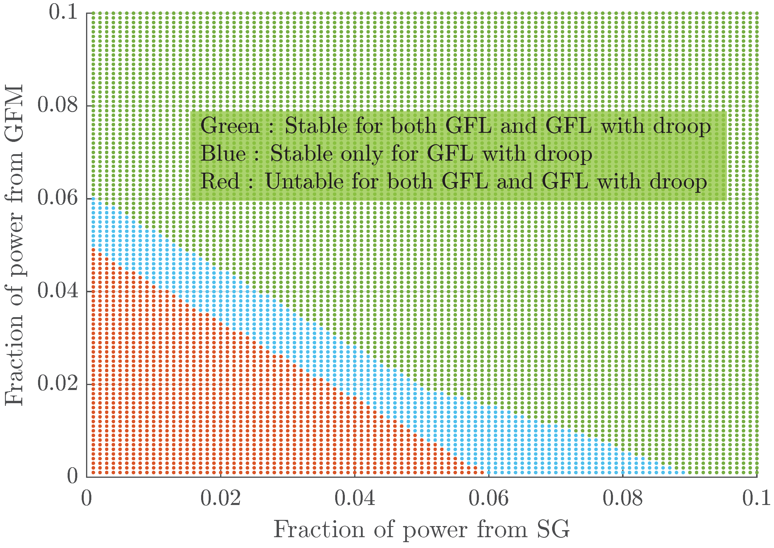
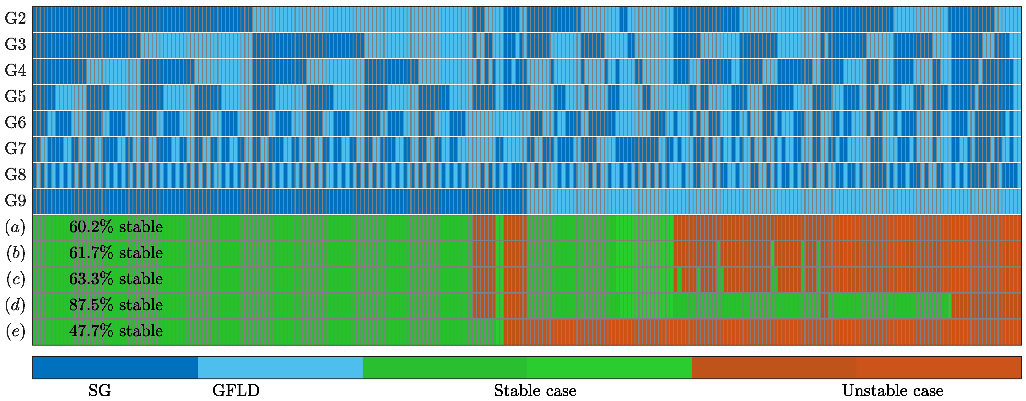
4.5. Fractional Replacement of SGs with IBRs

We studied the possibility of having IBRs with the existing SGs at each generator bus. Instead of completely shutting down the SGs, here, all the SGs at Gen 2–9 were partially replaced with both Droop-GFM and GFL inverters. The system’s stability is shown in Figure 10 when the total power from each plant was generated from SGs, Droop-GFM, and GFL/GFLD systems. For simplicity, the proportions of the generation assets were kept consistent across all generator buses in a given case. Considering the similarity of Droop-GFM and VOC-GFM for stability shown in Section 4.2, the analysis following uses the Droop-GFM.

Observation: When SGs or GFM inverters were connected at each generator bus, i.e., providing a voltage source at every bus, the system remained stable even with >90% of total generation from GFL or GFLD inverters, even approaching $95\%$ with GFLD and GFM, as illustrated in Figure 10. Notable is that the system stability with GFMs (stability trend around the y axis) is now comparable to the one with SGs (around the x axis), implying the marginal impact of system inertia on stability when GFM IBRs are distributed throughout the system. It motivates us to connect the GFM IBRs in a distributed manner to stabilize the grid rather than having one large plant in one place. The wide deployment of GFM assets at partial scales of the entire IBR generation might also be more cost-effective because the GFM assets would require more functionalities and meet higher standards than GFL IBRs. Having GFM assets distributed throughout a system would also be beneficial for grid resilience, since it would allow flexible islanded operation against contingencies and GFM inverter-driven black starts [36,37].

4.6. Impact of IBR Control Parameters on Stability

Tuning the control parameters of IBRs is a critical task in power system planning and operation, during both initial commissioning and operation. Through case studies, we discuss the effect of some control parameters on the small-signal stability to illustrate general trends.

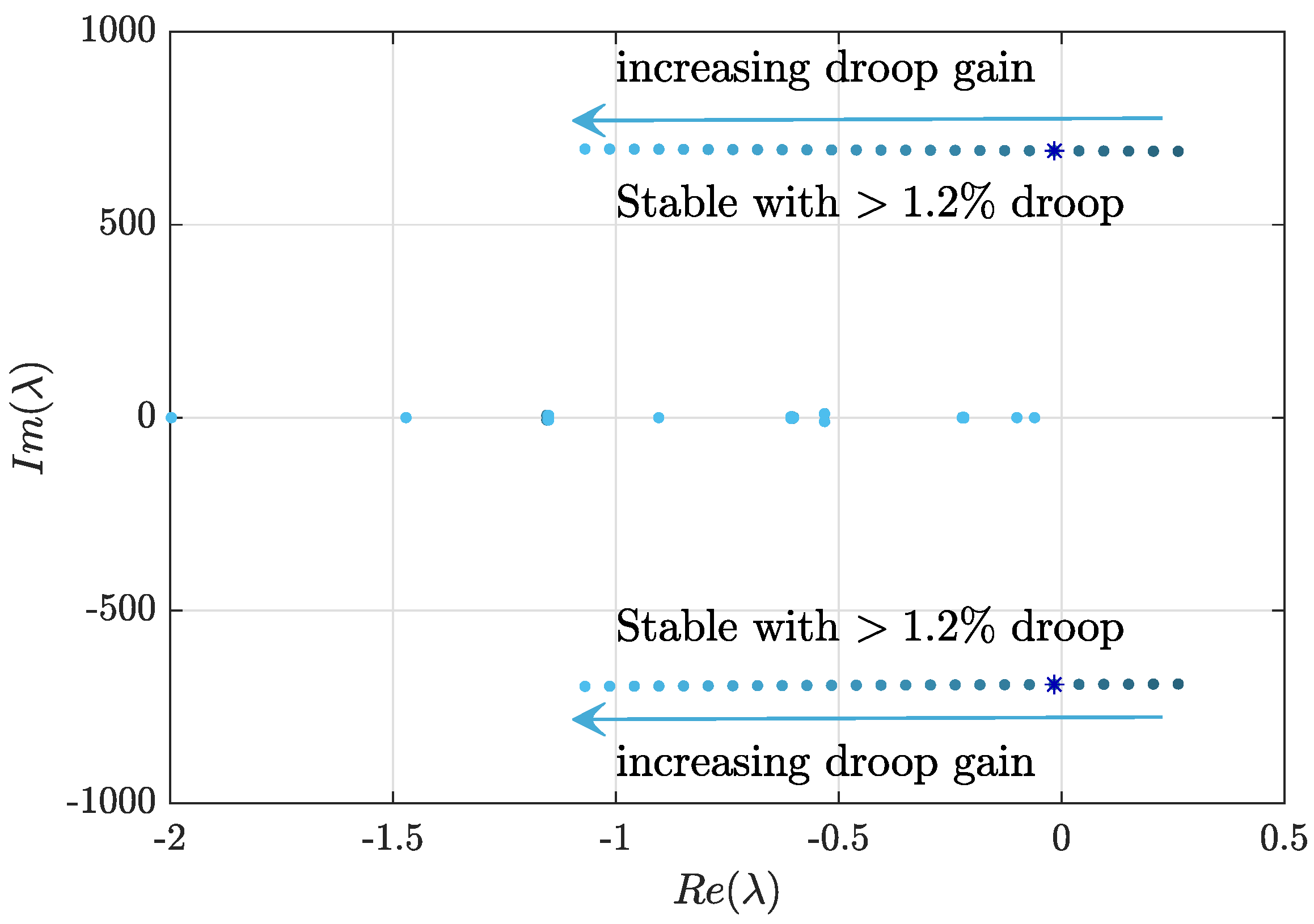
4.6.1. Effect of Droop Gain of GFLD Inverters

For this scenario, Gen 2–6 and Gen 8–9 were replaced with GFLD inverters, and the rest of the plants were SGs. In this case, the droop gain ($k_{\omega }$) in (7a) for all the GFLDs varied from $1\%$ p.u. to $5\%$ p.u. for a small-signal stability study. Figure 11 shows the changes of the system eigenvalues around the right-half plane for decreasing the droop gain in (7a). In this scenario, the same frequency deviation caused less change in active power, which shifted the real part of the eigenvalue toward the right of the real plane and, as a result, destabilized the system after the droop gain was decreased below a certain value, 1.2% in this case.

Note: It is known that for Droop-GFM inverters, increasing the droop gain causes instability when the frequency is drooped with the difference between the active power reference and the active power generation [38]. For GFLD inverters, on the other hand, the active power reference is drooped with the frequency deviation. So, decreasing the droop gain causes instability for GFLD inverters, consistent with the understanding of stability with GFM.

4.6.2. Impact of PLL Controller Parameters of GFLD Inverters on Stability

It has been reported that the PLL controller parameters affect the stability of GFL inverters and therefore might cause instability in a power system. Here, Gen 2–6 and Gen 8–9 were replaced with GFLD inverters in the original 39-bus system. Figure 12 shows that increasing the proportional controller gain ($k_{PLL}^p$) in the PI controller used in the PLL could cause small-signal instability.

Observation: Increasing the proportional controller gain decreases the bandwidth of the PI controller, causing the PLL dynamic to be slower, and as a result, instability can appear. In addition, though the results are not explicitly shown due to the space constraint, the sensitivity of the PLL controller parameters on small-signal stability for GFLD inverters is greater than for GFL inverters. As the frequency output of the PLL is further used to decide the active power reference, the PI controller inside the PLL has direct involvement in the system stability for GFLD inverters.

4.7. Impact of SG Inertia and Role of GFM Inverter

As shown in (2), the mechanical inertia (H) directly impacts the frequency dynamics of an SG. Therefore, it can affect the system stability, especially in systems with high penetrations of GFL inverters that need reliable terminal voltage. To investigate this, a stability analysis with varying inertia constants was conducted. Figure 13a–e display the exhaustive stability assessment, where the inertia constants of the SGs were scaled from a factor of 0.2 to 5. For simplicity, the inertia constants were scaled with the same factor for all SGs in each case. In the result, the variation in the inertia affected the system stability; interestingly, whether it was scaled down or up, the system stability did not improve but degraded, which matches a previous observation reported in [39]. Also notable is that cases with stability differed with the direction of the inertia scaling, which impedes deriving a generalized conclusion.

On the other hand, Figure 13f,g show an example where the variation in the inertia might not largely affect the stability in some cases; inertia scaling of Gen 10 at bus 39 by factors of 0.1 and 10, accounting for the majority of the system inertia (64% in the model) to model the interconnection, did not affect the system stability. To examine the impact of GFM inverters under varying inertia, Figure 13h shows the stability assessment with GFM inverters in place of GFL inverters with the inertia scaled by 0.5. Compared to the stability of the scenario with the inertia scaled by a factor of 0.5 and with GFL inverters, shown in Figure 13c, the result shows that the GFM inverters mitigated instability when the inertia decreased, suggesting the benefit of GFMs in the course of the energy mix transition. Overall, this study implies that simplistic insights cannot be derived regarding system inertia. Therefore, an in-depth study is needed to understand the system behavior in a specific setup and to ensure stability for power systems with high penetrations of IBRs, e.g., by system operators.

4.8. Impact of STATCOM and SC on Stability

Next, we studied the impact of the reactive power support elements, mainly STATCOM and SC, on the small-signal stability, along with IBR penetrations. First, when Gen 2–9 were either GFL IBRs or SGs (Scenario (a) in Section 4.2), this study investigated whether the presence of SCs or STATCOMs with GFL IBRs could improve the stability of the unstable cases. As shown in Figure 14a, all the unstable cases with SGs and GFL inverters were used as the baseline here, being the same as what is shown in Figure 6. As shown in Figure 14b–d, a STATCOM near Gen 6, 7, or 9 could make some of the previously unstable cases stable. Also, the effect of the SC near Gen 6, 7, or 9 is shown in Figure 14e–g.

Observation: In the presence of an SC, a greater number of cases become stable than in the presence of a STATCOM. This motivates us to use the retired SGs as SCs in the future grid.

4.9. Impact of Line Impedance on Stability

In the presence of the IBRs, the impact of the line impedance on the small-signal stability was studied. For this study, Gen 2–9 were replaced with SGs or GFLD inverters in all possible combinations. Considering the most critical generator location, i.e., Gen 9, a line impedance near Gen 9, from bus 28 to 29 (highlighted in Figure 5), was scaled by a factor of $0.01$ to 10, and the stability was observed. Line scaling can represent installing tie lines to strengthen the connections or disconnecting ones. As shown in Figure 15, decreasing the line impedance marginally improved the system stability, especially in cases with Gen 9 replaced with GFLD inverters. This result indicates the potential use of tie lines for grid stabilization in case this is more reasonable than installing a GFM inverter. Two extreme cases are also shown in Figure 15d,e. When the line impedance was very low, equivalent to having two buses electrically nearby, the stability significantly improved, confirming the criticality of the line. On the other hand, having a significantly higher impedance line, equivalent to removing the line from a contingency—potentially leading to a weak grid if no alternative low-impedance path exists—would cause more instability.

Key takeaways from the stability analyses in Section 4 are summarized in

Table 2. Takeaways from stability analysis of power systems with IBRs and grid-support technologies.

Items	Takeaways
GFL and GFLD inverter	It is not practical to have a stable grid with the majority of SGs replaced with only grid-following inverters. The study reconfirms the need for voltage sources, i.e., GFM IBRs. Having grid-support functions in GFL IBRs improves the system stability, but it cannot guarantee system stability.
GFM inverter	It is critical to have GFM IBRs for stability in the IBR-dominant grid. However, having all IBRs with GFM control would not be necessary or practical, considering the additional engineering and cost needed.
Co-existence of SG, GFM, and GFL	Having voltage sources (SG or GFM) at fractional scales, distributed throughout the grid, would help retain system stability with the majority of IBRs run by conventional GFL controls, elucidating a practical approach for future grid stabilization.
SC and STATCOM	Having SC or STATCOM at nonvoltage source buses can improve stability in GFL-heavy grids, which confirms their effectiveness. They differ in grid stabilization due to their fundamental difference.
Other grid parameters	The role of machine inertia in system stability of high IBR penetration power systems is not clear, suggesting the necessity of further study. Network impedance affects system stability, especially in IBR-heavy grids, requiring attention in system planning and contingency analysis.

.

5. Conclusions and Future Works

With increasing IBR penetration and the retirement of SGs, power grids face growing challenges in maintaining stability. To support this transition, GFM controls, alongside other supporting technologies, are essential. Based on an exhaustive small-signal stability analysis of the IEEE 39-bus system incorporating state-of-the-art inverter models, this study revealed that the generator type plays a critical role in system stability, particularly when vulnerable buses are replaced with GFL IBRs. By providing local frequency and voltage regulation, GFM IBRs located at critical buses can stabilize the system even when they account for only a small portion of the total generation capacity. The analysis also shows that the system inertia significantly impacts stability, especially when the generation mix lacks diversity (e.g., only one generator type per bus). However, increasing the SG inertia is not always beneficial and can degrade system stability, a finding that aligns with the existing literature. Notably, distributing GFM units across the network, in contrast, reduces sensitivity to inertia variations and can enhance overall stability. Furthermore, the study confirms the sensitivity of system stability to inverter control parameters. While this work primarily focused on one specific parameter, the interactions among various control settings and system-level designs are equally important but complex, warranting future investigation. Finally, the role of reactive power support devices, such as STATCOMs and SCs, was examined, showing distinct impacts when deployed alongside GFL IBRs. The influence of tie-line reinforcement on stability was also assessed. Together, these findings offer valuable insights into the small-signal stability of future bulk power systems under high IBR penetration.

Future works include (a) assessing the effect of different types of control implementation for GFL IBRs, (b) comparing the impact of different GFM types, such as virtual machine and matching control, and (c) analyzing the interoperability of different GFL and GFM controls with legacy assets to stabilize a grid.

References

1. Kroposki, B. UNIFI Specifications for Grid-Forming Inverter-Based Resources (v. 2); Technical Report; National Renewable Energy Laboratory (NREL): Golden, CO, USA, 2024.
2. Chen, Y.; Shi, K.; Chen, M.; Xu, D. Data center power supply systems: From grid edge to point-of-load. IEEE J. Emerg. Sel. Top. Power Electron. 2022, 11, 2441–2456. [Google Scholar] [CrossRef]
3. Xu, S.; Xue, Y.; Chang, L. Review of power system support functions for inverter-based distributed energy resources-standards, control algorithms, and trends. IEEE Open J. Power Electron. 2021, 2, 88–105. [Google Scholar] [CrossRef]
4. Huber, J.E.; Kolar, J.W. Applicability of solid-state transformers in today’s and future distribution grids. IEEE Trans. Smart Grid 2017, 10, 317–326. [Google Scholar] [CrossRef]
5. Lin, Y.; Eto, J.H.; Johnson, B.B.; Flicker, J.D.; Lasseter, R.H.; Villegas Pico, H.N.; Seo, G.S.; Pierre, B.J.; Ellis, A. Research Roadmap on Grid-Forming Inverters; Technical Report; National Renewable Energy Lab.(NREL): Golden, CO, USA, 2020.
6. Milano, F.; Dörfler, F.; Hug, G.; Hill, D.J.; Verbič, G. Foundations and challenges of low-inertia systems. In Proceedings of the Power Systems Computation Conference, Dublin, Ireland, 11–15 June 2018; pp. 1–25. [Google Scholar]
7. Du, W.; Liu, Y.; Tuffner, F.K.; Huang, R.; Huang, Z. Model Specification of Droop-Controlled, Grid-Forming Inverters (GFMDRP_A); Technical Report; Pacific Northwest National Laboratory (PNNL): Richland, WA, USA, 2021.
8. Seo, G.S.; Colombino, M.; Subotic, I.; Johnson, B.; Gross, D.; Dörfler, F. Dispatchable virtual oscillator control for decentralized inverter-dominated power systems: Analysis and experiments. In Proceedings of the IEEE Applied Power Electronics Conference and Exposition (APEC), Anaheim, CA, USA, 17–21 March 2019; pp. 561–566. [Google Scholar]
9. Awal, M.; Yu, H.; Husain, I.; Yu, W.; Lukic, S.M. Selective harmonic current rejection for virtual oscillator controlled grid-forming voltage source converters. IEEE Trans. Power Electron. 2020, 35, 8805–8818. [Google Scholar] [CrossRef]
10. Du, W.; Achilles, S.; Ramasubramanian, D.; Hart, P.; Rao, S.; Wang, W.; Nguyen, Q.; Kim, J.; Zhang, Q.; Liu, H.; et al. Virtual Synchronous Machine Grid-Forming Inverter Model Specification (REGFM_B1); Technical Report; National Renewable Energy Laboratory (NREL): Golden, CO, USA, 2024.
11. Arghir, C.; Jouini, T.; Dörfler, F. Grid-forming control for power converters based on matching of synchronous machines. Automatica 2018, 95, 273–282. [Google Scholar] [CrossRef]
12. Ali Khan, M.Y.; Liu, H.; Yang, Z.; Yuan, X. A comprehensive review on grid connected photovoltaic inverters, their modulation techniques, and control strategies. Energies 2020, 13, 4185. [Google Scholar] [CrossRef]
13. Markovic, U.; Stanojev, O.; Aristidou, P.; Vrettos, E.; Callaway, D.; Hug, G. Understanding Small-Signal Stability of Low-Inertia Systems. IEEE Trans. Power Syst. 2021, 36, 3997–4017. [Google Scholar] [CrossRef]
14. Ding, L.; Lu, X.; Tan, J. Comparative Small-Signal Stability Analysis of Grid-Forming and Grid-Following Inverters in Low-Inertia Power Systems. In Proceedings of the 47th Annual Conference of the IEEE Industrial Electronics Society, Toronto, ON, Canada, 13–16 October 2021; pp. 1–6. [Google Scholar] [CrossRef]
15. He, X.; Pan, S.; Geng, H. Transient Stability of Hybrid Power Systems Dominated by Different Types of Grid-Forming Devices. IEEE Trans. Energy Convers. 2022, 37, 868–879. [Google Scholar] [CrossRef]
16. Johnson, B.; Sinha, M.; Ainsworth, N.; Dörfler, F.; Dhople, S. Synthesizing Virtual Oscillators to Control Islanded Inverters. IEEE Trans. Power Electron. 2015, 31, 6002–6015. [Google Scholar] [CrossRef]
17. Siraj Khan, M.M.; Lin, Y.; Johnson, B.; Sinha, M.; Dhople, S. Stability Assessment of a System Comprising a Single Machine and a Virtual Oscillator Controlled Inverter with Scalable Ratings. In Proceedings of the 44th Annual Conference of the IEEE Industrial Electronics Society, Washington, DC, USA, 21–23 October 2018; pp. 4057–4062. [Google Scholar] [CrossRef]
18. Johnson, B.; Rodriguez, M.; Sinha, M.; Dhople, S. Comparison of virtual oscillator and droop control. In Proceedings of the IEEE Workshop on Control and Modeling for Power Electronics, Stanford, CA, USA, 9–12 July 2017; pp. 1–6. [Google Scholar]
19. Arévalo-Soler, J.; Sánchez-Sánchez, E.; Prieto-Araujo, E.; Gomis-Bellmunt, O. Impact analysis of energy-based control structures for grid-forming and grid-following MMC on power system dynamics based on eigenproperties indices. Int. J. Electr. Power Energy Syst. 2022, 143, 108369. [Google Scholar] [CrossRef]
20. Kenyon, R.W.; Hoke, A.; Tan, J.; Hodge, B.M. Grid-following inverters and synchronous condensers: A grid-forming pair? In Proceedings of the 2020 Clemson University Power Systems Conference, Clemson, SC, USA, 10–13 March 2020; pp. 1–7. [Google Scholar]
21. Stiger, A.; Rivas, R.; Halonen, M. Synchronous condensers contribution to inertia and short circuit current in cooperation with STATCOM. In Proceedings of the IEEE PES GTD Grand International Conference and Exposition Asia, Bangkok, Thailand, 19–23 March 2019; pp. 955–959. [Google Scholar]
22. Hu, W.; Su, C.; Fang, J.; Chen, Z. Comparison study of power system small signal stability improvement using SSSC and STATCOM. In Proceedings of the 39th Annual Conference of the IEEE Industrial Electronics Society, Vienna, Austria, 10–13 November 2013; pp. 1998–2003. [Google Scholar] [CrossRef]
23. Liu, Y.; Yang, S.; Zhang, S.; Peng, F.Z. Comparison of synchronous condenser and STATCOM for inertial response support. In Proceedings of the IEEE Energy Conversion Congress and Exposition, Pittsburgh, PA, USA, 14–18 September 2014; pp. 2684–2690. [Google Scholar] [CrossRef]
24. Gross, D.; Colombino, M.; Brouillon, J.S.; Dörfler, F. The Effect of Transmission-Line Dynamics on Grid-Forming Dispatchable Virtual Oscillator Control. IEEE Trans. Control Netw. Syst. 2019, 6, 1148–1160. [Google Scholar] [CrossRef]
25. Rui, W.; Qiuye, S.; Dazhong, M.; Xuguang, H. Line Impedance Cooperative Stability Region Identification Method for Grid-Tied Inverters Under Weak Grids. IEEE Trans. Smart Grid 2020, 11, 2856–2866. [Google Scholar] [CrossRef]
26. Li, D.; Yang, S.; Huang, W.; He, J.; Yuan, Z.; Yu, J. Optimal Planning Method for Power System Line Impedance Based on a Comprehensive Stability Margin. IEEE Access 2021, 9, 56264–56276. [Google Scholar] [CrossRef]
27. Lin, Y.; Seo, G.S.; Vijayshankar, S.; Johnson, B.; Dhople, S. Impact of Increased Inverter-based Resources on Power System Small-signal Stability. In Proceedings of the IEEE Power & Energy Society General Meeting, Washington, DC, USA, 26–29 July 2021; pp. 1–5. [Google Scholar]
28. Australian Energy Market Operator. Application of Advanced Grid-scale Inverters in the NEM. In White Paper; Australian Energy Market Operator: Victoria, Australia, 2021. [Google Scholar]
29. Hiskens, I.A. IEEE PES Task Force on Benchmark Systems for Stability Controls; Technical Report; IEEE Power & Energy Society: Piscataway, NJ, USA, 2013. [Google Scholar]
30. Sauer, P.W.; Pai, M.A. Power System Dynamics and Stability; Wiley Online Library: Hoboken, NJ, USA, 1998; Volume 101. [Google Scholar]
31. Teodorescu, R.; Liserre, M.; Rodriguez, P. Grid Converters for Photovoltaic and Wind Power Systems; John Wiley & Sons: Hoboken, NJ, USA, 2011. [Google Scholar]
32. Tayyebi, A.; Groß, D.; Anta, A.; Kupzog, F.; Dörfler, F. Frequency Stability of Synchronous Machines and Grid-Forming Power Converters. IEEE J. Emerg. Sel. Top. Power Electron. 2020, 8, 1004–1018. [Google Scholar] [CrossRef]
33. Ali, Z.; Christofides, N.; Hadjidemetriou, L.; Kyriakides, E.; Yang, Y.; Blaabjerg, F. Three-phase phase-locked loop synchronization algorithms for grid-connected renewable energy systems: A review. Renew. Sustain. Energy Rev. 2018, 90, 434–452. [Google Scholar] [CrossRef]
34. Bahrani, B. Power-synchronized grid-following inverter without a phase-locked loop. IEEE Access 2021, 9, 112163–112176. [Google Scholar] [CrossRef]
35. Pai, M. Energy Function Analysis for Power System Stability; Springer Science & Business Media: Berlin/Heidelberg, Germany, 2012. [Google Scholar]
36. Zhao, J.; Zhang, Q.; Ziwen, L.; Xiaokang, W. A distributed black-start optimization method for global transmission and distribution network. IEEE Trans. Power Syst. 2021, 36, 4471–4481. [Google Scholar] [CrossRef]
37. Sawant, J.; Seo, G.S.; Ding, F. Resilient Inverter-Driven Black Start with Collective Parallel Grid-Forming Operation. In Proceedings of the IEEE Power & Energy Society Innovative Smart Grid Technologies Conference (ISGT), Washington, DC, USA, 16–19 January 2023; pp. 1–5. [Google Scholar]
38. Du, W.; Chen, Z.; Schneider, K.P.; Lasseter, R.H.; Nandanoori, S.P.; Tuffner, F.K.; Kundu, S. A Comparative Study of Two Widely Used Grid-Forming Droop Controls on Microgrid Small-Signal Stability. IEEE J. Emerg. Sel. Top. Power Electron. 2019, 8, 963–975. [Google Scholar] [CrossRef]
39. Lin, Y.; Johnson, B.; Gevorgian, V.; Purba, V.; Dhople, S. Stability assessment of a system comprising a single machine and inverter with scalable ratings. In Proceedings of the North American Power Symposium (NAPS), Morgantown, WV, USA, 17–19 September 2017; pp. 1–6. [Google Scholar]
Figure 1. Generic machine and inverter models for analysis: (a) synchronous generator model with AVR, PSS, and governor; (b) inverter model with measured voltage and current used as input for the controllers and the inverter switching signals generated by the controller.
Energies 18 03645 g001
Figure 2. Primary control diagram for the Droop-GFM inverter.
Energies 18 03645 g002
Figure 3. Primary control diagram of the VOC-GFM inverters.
Energies 18 03645 g003
Figure 4. Simplified control diagram of GFL inverters.
Energies 18 03645 g004
Figure 5. IEEE 39-bus–10-machine New England power system.
Energies 18 03645 g005
Figure 6. Power system stability with different combinations of voltage sources (SG, Droop-GFM, or VOC-GFM) and current sources (GFL or GFLD). Stable and unstable cases (darker shades are used for max real eigenvalue with greater absolute value) when Gen 2–9 are replaced with different types of generation: (a) SG and GFL, (b) SG and GFLD, (c) Droop-GFM and GFL, (d) Droop-GFM and GFLD, (e) VOC-GFM and GFL, and (f) VOC-GFM and GFLD.
Energies 18 03645 g006
Figure 7. Stability rates for different generators replaced with GFL inverters and the rest of Gen 2–9: (a) SG and GFL, (b) SG and GFLD, (c) Droop-GFM and GFL, (d) Droop-GFM and GFLD, (e) VOC-GFM and GFL, and (f) VOC-GFM and GFLD.
Energies 18 03645 g007
Figure 8. Participation factor for the unstable mode when Gen 2–9 are replaced with GFL inverters.
Energies 18 03645 g008
Figure 9. Stability with GFM IBR penetration levels for all six scenarios explained in Section 4.2.
Energies 18 03645 g009
Figure 10. Stable and unstable cases when the total power generation is coming fractionally from SG, GFM, and GFL/GFLD for all the Gen 2–9. Here, fractions of power generation from SG and GFM are shown in the x axis and y axis, respectively, and the rest of the generation is from GFL/GFLD.
Energies 18 03645 g010
Figure 11. Eigenvalues with change in GFLD droop gain (1% p.u.–5% p.u.) after replacing Gen 2–6 and Gen 8–9 with the GFLD inverters. notes the stability boundary.
Energies 18 03645 g011
Figure 12. Eigenvalues with change in the proportional controller gain of the PLL PI controller in the GFLD inverters. The controller gain is scaled from 0.1 to 2 times its nominal value.
Energies 18 03645 g012
Figure 13. Stability impact of SG inertia variations with different inverter penetrations (darker shades are used for max real eigenvalue with greater absolute value): (a) inertia of all SGs scaled by 1 (baseline, GFL inverters replace SGs), (b) by 0.2, (c) by 0.5, (d) by 2, (e) by 5; (f) inertia of Gen 10 scaled by 0.1 with the inertia of the other SGs kept the same and GFLs, (g) by 10; (h) GFM inverters replacing GFLs with inertia of all SGs scaled by 0.5.
Energies 18 03645 g013
Figure 14. Stability assessment of unstable cases when Gen 2–9 are replaced with GFL inverters with a STATCOM or SC placed in a GFL bus: (a) no SC or STATCOM (baseline), (b) STATCOM near Gen 6, (c) STATCOM near Gen 7, (d) STATCOM near Gen 9, (e) SC near Gen 6, (f) SC near Gen 7, and (g) SC near Gen 9.
Energies 18 03645 g014
Figure 15. Effect of line impedance on the small-signal stability when Gen 2–9 are replaced with SGs and GFLD inverters (darker shades are used for max real eigenvalue with greater absolute value). The line impedance between bus 28 and 29 is scaled with (a) 1 (baseline), (b) 0.9, (c) 0.75, (d) 0.01 (equivalent to having bus 28 and 29 very nearby), and (e) 10 (equivalent to removing the line).
Energies 18 03645 g015