The Impact of VAT Preferential Policies on the Profitability of China’s New Energy Power Generation Industry

Abstract

To achieve climate goals and promote clean energy, China has introduced preferential VAT policies to promote the development of renewable energy power generation industries, but their actual impact on corporate profitability remains underexplored. This study innovatively applies a DID approach, enhanced with PSM and dynamic modeling, to evaluate the causal effects of VAT incentives on firm ROE. Using panel data from 98 listed power generation companies between 2010 and 2024, this study distinguishes treatment effects across the wind, solar, and hydrogen sectors, revealing significant heterogeneity. Unlike prior studies, it further investigates time-lagged impacts and fiscal efficiency indicators to assess policy sustainability. Results show that VAT incentives significantly enhance ROE for wind and solar firms, while the hydrogen sector exhibits weaker responses. These findings not only confirm the effectiveness of targeted tax incentives but also offer new insights for refining fiscal policies to better support sector-specific transitions toward renewable energy. This study provides empirical evidence for the design of China’s fiscal energy policy to maximize the growth of the renewable energy sector. More broadly, this study provides lessons for global green transition policies, illustrating how well-designed fiscal incentives can support sustainable energy development worldwide.

1. Introduction

Electricity is the foundation of a country’s development and is at the core of the social chain. With the progress of the times, power generation enterprises provide many types of power generation, such as thermal power generation, waterpower generation, and new energy generation. Among them, thermal power generation is more significant to the social pollution of the atmosphere, and water conservancy power generation is also destructive to local ecological culture.

Therefore, new energy power generation is being developed globally. As of the end of June 2024, new energy met more than 90% of the world’s incremental power demand. Further, China’s new energy power generation installed capacity reached 1.653 billion kilowatts, an increase of 25% year-on-year, accounting for about 53.8% of China’s total installed power generation, of which 427 million kilowatts were of hydroelectricity, 467 million kilowatts were of wind power, 714 million kilowatts were of solar power generation installed capacity, and 45.3 million kilowatts were of biomass power generation installed capacity. The combined installed capacity of wind power and photovoltaic power generation (1.18 billion kilowatts) has exceeded the installed capacity of coal power (1.17 billion kilowatts).

Current research on tax incentives and the new energy generation industry focuses on the relationship between tax formulation and energy transition [1,2] and the relationship between tax incentives and industry forgery and innovation, while less attention has been paid to the study of tax incentives on the financial performance of the new energy industry [3,4] (Figure 1).

The financial performance of the power generation industry is measured using two main figures: return on total assets and return on net assets. The return on total assets is related to the total profit and total assets of the enterprise for the year [5,6]. The return on net assets is related to the net profit and net assets of the enterprise for the year, both of which reflect the enterprise’s ability to generate profits from all assets, and a higher level of this indicator indicates a higher level of performance [7].

The recent literature has also emphasized the need to align renewable energy policies with broader societal goals, such as the development of sustainable communities. This concept highlights the integration of environmental, economic, and social dimensions of sustainability [8]. Enterprises are subsidized through tax incentives enacted by the state, which, with reasonable external policy interventions, can lead to higher profits and thus higher performance levels [9].

In parallel, the pragmatic model of sustainability has gained traction in policy-oriented research. This model moves beyond idealistic or purely ecological framings of sustainability by promoting adaptive, flexible, and context-sensitive solutions. It suggests that policies such as VAT incentives should not only aim to reduce emissions or boost financial returns but also consider institutional feasibility, social acceptance, and fiscal sustainability over time. As such, incorporating these frameworks provides a more holistic understanding of how fiscal tools like tax incentives can contribute to a just and enduring green transition, especially in emerging economies like China [10].

Therefore, developed countries, such as the United States of America, have formulated corresponding preferential policies to meet the conditions of solar power generation enterprises operating in their first ten years in order to give a certain degree of tax relief [11] and also for new energy power generation enterprises to implement the “R&D expenses plus deduction” and “income tax” double policy concessions [12]. The German government implements an investment tax credit policy for photovoltaic power generation enterprises, and the Japanese government adds up the costs incurred by enterprises due to the purchase of wind and photovoltaic power generation equipment.

Tax incentives have a profound impact on the development of the new energy power generation industry, and the promise of these tax incentives have brought more investment in the new energy power generation industry; however, tax incentives also have related economic defects [13], i.e., they may distort the structure of the industrial chain and reduce technological upgrading, especially if the incentives are only focused on a certain part of the industrial chain [14]. Therefore, this paper examines the impact of value-added tax (VAT) incentives on the ROE (ROE) of listed companies as an example.

This paper chooses new energy power generation listed companies as the sample for its study. The main reasons for the selection are as follows: first, the scale of investment in China’s power industry continued to expand from 2014 to 2024, and in 2024 alone, the national full-caliber installed power generation capacity reached 3.35 billion kilowatts, a year-on-year increase of 14.6%. Among the types of power generation, the installed capacity of new energy power generation (including wind power, solar power, and biomass power) reached 1.45 billion kilowatts, exceeding the installed scale of thermal power for the first time. At the same time, the installed capacity of thermal power was 1.44 billion kilowatts [15], of which 1.19 billion kilowatts were from coal power, up 2.6% year-on-year, and the proportion of total installed capacity dropped to 35.7%, down 4.2 percentage points year-on-year. The installed capacity of non-fossil energy power generation was 1.95 billion kilowatts, up 23.8% year-on-year, accounting for 58.2% of the total installed capacity, an increase of 4.3 percentage points from the end of the previous year (Figure 2).

However, some enterprises are still showing losses, which shows that China’s new energy enterprises have great market potential but low profitability [16]. This is quite different from their international counterparts and is worth studying. Second, in the process of economic structural transformation and upgrading, intensive institutional reforms and dynamic policy regulation have a significant impact on the market. Among them, the tax incentive system, with tax exemption, tax refunds, and export tax rebates at its core, has become a key institutional arrangement to promote the development of the new energy industry. Focusing on policy practice in the field of value-added tax, China has implemented differentiated preferential measures for the four strategic areas of wind power, photovoltaic power generation, nuclear energy, and new energy vehicles. These policies not only have a clear industry orientation but also show a step-by-step feature in their implementation cycle and implementation intensity [17], which provides a realistic basis for conducting multi-dimensional quantitative evaluation of policy effects.

The aim of the study is to examine the impact of tax incentives on the profitability of China’s new energy power generation industry.

Although previous studies have widely applied the DID approach to assess the impact of tax incentives on firm performance, this study advances the existing literature in three important ways. First, we disaggregate the new energy power generation sector into wind, solar, and hydrogen sub-industries and estimate sector-specific effects using subgroup DID models, capturing heterogeneous responses. Second, we adopt a dynamic DID framework to trace annual changes in ROE for up to five years post-intervention, identifying the time-varying marginal effects of VAT incentives. Third, we evaluate the sustainability of such incentives by introducing firm-level tax dependency and annual fiscal return on investment (ROI), offering a fiscal efficiency perspective often overlooked in prior research. These innovations allow the present study to move beyond static evaluations and provide targeted, policy-relevant insights for China’s green transition.

Our research hypotheses are as follows:

H1. 

VAT incentives significantly enhance the profitability of new energy firms by reducing tax burdens and improving financial performance.

H2. 

VAT incentives create market distortions, leading to resource misallocation and overcapacity in the new energy sector, thereby negatively impacting long-term industry sustainability.

2. Literature Review

The last decade has witnessed unprecedented growth in new energy sources—primarily wind, solar, and other renewables—driven by sharp cost declines and proactive energy policies worldwide [18]. Globally, renewables now dominate new power capacity additions, far outpacing fossil fuels. China has emerged as the world leader in renewable power deployment: between 2019 and 2024, China alone is expected to account for about 40% of the world’s growth in renewable capacity [19]. This surge is attributed to improved grid integration, falling curtailment of wind/solar, and strong government targets and incentives.

Other countries, such as the United States, India, and those in the EU, have also set ambitious renewable energy goals as part of their climate commitments. In fact, a global study [20,21] found that countries focusing on expanding renewables achieved significantly greater CO₂ emissions reductions than those prioritizing nuclear expansion, indicating that renewables have delivered faster decarbonization in practice.

Policy evolution has been crucial in scaling up new energy. Early renewable pioneers in Europe (Germany, Spain, Denmark, etc.) demonstrated the impact of stable financial incentives like feed-in tariffs in the 2000s, which led to exponential growth of wind and solar installations [22]. As markets matured, many countries transitioned to competitive bidding schemes (auctions) to procure renewable power at lower costs [23]. For example, large-scale solar PV auction prices fell to record lows (below USD 0.02/kWh in some cases by 2020) as developers worldwide responded to these policy signals [24,25,26].

Other policy tools have included renewable portfolio standards [27,28] (mandating utilities to source a percentage of power from renewables), net metering and tax credits to spur distributed generation, and targeted grants or R&D support for emerging technologies like battery storage and hydrogen. Interestingly, their study noted that tax incentives alone are not sufficient—they work best when combined with robust deployment policies (e.g., auctions, mandates) to realize renewable projects [29,30].

Recent quantitative research provides mixed evidence. On the one hand, reducing taxes should improve a company’s cash flow and profitability, thereby attracting more entrants and investment. Yi & Feiock [31] found that, overall, tax reductions (including VAT cuts) have positive effects on the green energy sector’s growth in China, alleviating financial burdens and boosting firm performance. In their empirical analysis of 100 listed green energy companies, they observed that after tax reductions, companies’ operating costs dropped and profitability (e.g., ROE) increased, enabling higher R&D spending and efficiency improvements. These findings support the view that VAT incentives and similar tax breaks can bolster the sector by improving short-term financial metrics and capacity for innovation [32,33,34,35].

On the other hand, a more nuanced picture emerges when examining differential impacts across firms and over time. In other words, firms benefiting from VAT refunds were less profitable than those without the incentive once other factors were controlled for [36]. Qi et al. [37] attributed this unexpected result to distortions and overcapacity: the tax breaks stimulated a rush of investment and expansion in certain segments of the renewable industry [38] (notably solar manufacturing), leading to oversupply, price wars, and reduced profit margins. Essentially, the VAT incentive, by lowering costs, may have encouraged too many firms to scale up too quickly, undermining profitability—a classic case of an industrial policy overshooting its mark [39].

They also observed a time lag in effects, with the negative impact on ROE becoming evident a few years after the policy’s implementation and varying over time [40]. This dynamic effect suggests that the initial boost provided by tax incentives can transform into long-term competitive pressure as more players enter the market, as explained by Liu et al. [41]. Jafari et al. [42] evaluated China’s VAT refund policy for renewable power firms by comparing treated firms (those receiving VAT incentives) with a control group of firms not receiving such incentives. Counterintuitively, they found that the VAT incentives decreased the ROE of the treated new energy firms, which had an ROE 4.7% lower than the control group on average. These seemingly contradictory findings reflect the complex nature of VAT policy effects—initial gains in liquidity may be offset by increased competition and declining marginal returns. Our study contributes to this debate by incorporating industry capacity utilization and R&D dynamics to clarify under which conditions VAT incentives enhance or hinder firm profitability. The Chinese experience thus offers a cautionary tale: tax incentives, while helpful, can induce market distortions if not paired with measures to prevent oversupply or if not phased out as technologies mature [42].

Energy policies rarely have uniform effects on all technologies; instead, different energy types often exhibit heterogeneous responses to the same policy. This heterogeneity stems from variations in technology cost structures, resource availability [43], market maturity, and institutional context. In the new energy domain, a recurring theme is that wind and solar power have responded more rapidly and vigorously to policy support than nuclear power or other less-mature low-carbon options [44]. On the global scale, the past decade’s policy-driven boom has been overwhelmingly concentrated on wind and solar.

For instance, Liu et al. [45] found that the effectiveness of renewable energy promotion policies was particularly strong for wind and solar energy, with much larger capacity increases in those categories compared to bioenergy or other renewables. The wind industry similarly had a rush (“installation boom”) in 2020 before the subsidy deadline, followed by a brief slowdown and then a transition to subsidy-free projects. Nuclear, however, was unaffected by these subsidy policy changes (since it never depended on feed-in tariffs in the same way) —its projects continued according to long-term plans, relatively insulated from short-term policy shifts [46].

3. Materials and Methods

3.1. Retrodynamics of Tax Incentives

To promote the rapid development of the new energy power generation industry, the state has successively promulgated a few tax incentives that are beneficial to the industry. These policies cover a variety of fields, from wind energy and solar energy to geothermal energy, and provide financial support to enterprises by reducing and exempting value-added tax and import taxes [47]. Since 2005, the implementation of the New Energy Law has provided legal protection for the new energy field and gradually introduced subsidies and tax exemption policies for photovoltaic and wind power projects [48]. These policies not only encourage investment and technological innovation in new energy enterprises but also lay the foundation for the rapid development of the entire industry [49].

However, as the policy effects gradually emerged, 2014 became a key time node. In that year, the implementation of the policy entered a new stage, especially in terms of further strengthening the support for the wind, solar, and hydrogen industries [50]. Based on this, this study takes 2014 as the split point and uses the double difference model (DID) to compare the changes before and after the implementation of the policy to evaluate the impact of tax incentives on the new energy power generation industry [51] (

Table 1. Overview of major tax and incentive policies affecting the new energy sector in China.

Year of Policy Implementation	Name of Policy	Field of Application	Thrust
2005	Implementation of the New Energy Law	Wind, solar, geothermal, etc.	A legal framework for new energy development has been established and the implementation of tax incentives for wind, solar, and geothermal energy has been promoted.
2005	VAT incentives for solar photovoltaic power generation	Solar photovoltaic power generation	Solar photovoltaic equipment enjoys VAT exemptions or reductions to encourage the development of the solar industry.
2007	Tax incentives for the wind power industry	Tidal	Wind power projects enjoy income tax exemptions and equipment import tax exemptions, promoting the rapid development of the wind power industry.
2009	Tax incentives for geothermal energy generation	Geothermal power	Geothermal energy projects enjoy tax support such as preferential value-added tax (VAT) and import tax exemptions to promote the development and utilization of geothermal energy resources.
2014	Tax incentives and support measures for the hydrogen industry	Hydrogen (gas)	The hydrogen industry is included in the scope of national energy policy support including the implementation of equipment imports tax exemptions and corporate income tax exemptions.
2015	Feed-in tariff subsidy policy and tax incentives for the photovoltaic industry	Solar photovoltaic power generation	Increase feed-in tariff subsidies for photovoltaic (PV) power generation, as well as increase VAT exemptions and other tax incentives for PV power generation equipment.
2017	Tax incentives for wind power industry strengthened	Tidal	Strengthen tax incentives for the wind power industry by providing corporate income tax exemptions and financial support for technology research and development.
2018	Hydrogen industry tax incentives expanded	Hydrogen (gas)	Expand the scope of tax incentives for the hydrogen industry and increase support for tax breaks for hydrogen R&D, production, and storage facilities.
2020	Tax incentives for the hydrogen industry further strengthened	Hydrogen (gas)	Further reduce the tax burden on the hydrogen industry, especially in terms of support for hydrogen storage and transportation technologies, including import duty exemptions.
2020	Import duty exemption and enterprise income tax incentives for wind and solar power generation equipment	Wind, solar	Continue to provide equipment import duty exemptions and corporate income tax exemptions for wind and solar power projects to support technological innovation and program expansion.

).

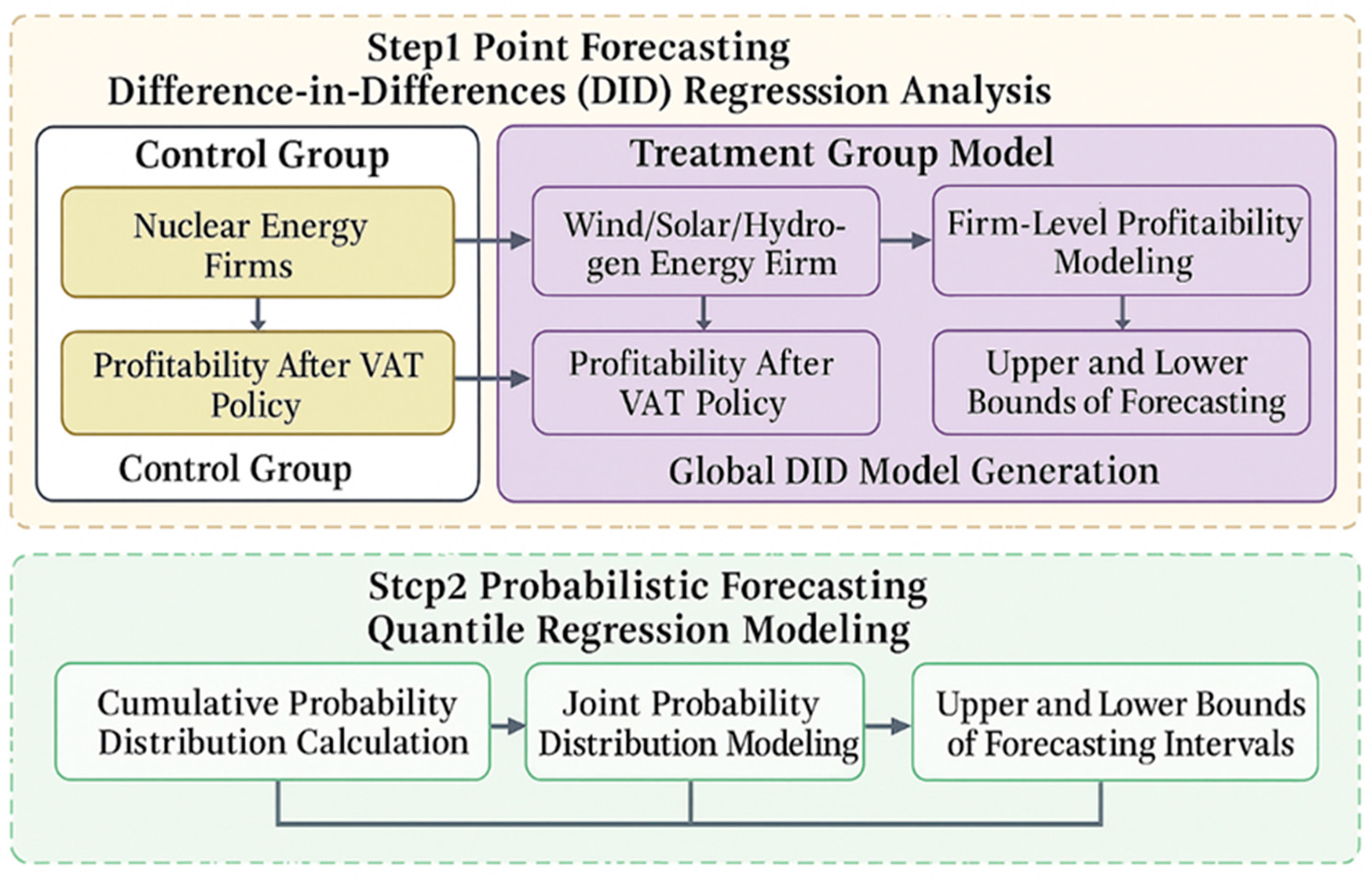
3.2. Difference-in-Difference Model

To evaluate the impact of tax incentives on the renewable energy power generation industry, this study uses a double difference model (DID) model to compare the differences in outcome variables between the “treatment group” and the “control group” before and after the implementation of the policy (2010–2014) and the period after the implementation of the policy (2015–2023) to identify the policy effect and effectively control the unobserved constant differences and common trends. In the early policy period, key tax incentives were gradually implemented in many areas of the renewable energy industry, including VAT exemptions and import tax concessions in wind, solar, and geothermal energy, as well as tax exemptions for nuclear power generation since the mid-1980s [52,53].

In contrast, the later policy period (2015–2023) saw a more comprehensive strengthening of tax incentives in the renewable energy sector, especially in photovoltaic and wind power projects, with further increases in VAT exemptions and corporate income tax incentives and greater subsidies for photovoltaic systems. It is worth noting that the policy for the hydrogen industry was further strengthened in 2018 and 2020, with more tax exemptions implemented to accelerate technological innovation and industrial development in the sector. The differences before and after the policy provide a strong basis for comparison of the DID model, which can effectively capture the gradual impact of tax incentives on the growth and technological progress of the new energy power generation industry.

To ensure that this hypothesis is valid, we conducted a parallel-trend test in the empirical analysis to confirm that there was no significant difference in the performance and innovation index trends between the treatment group and the control group before the policy was introduced. Specifically, the inter-group differences in the previous several periods before the policy were visually compared, and statistical tests were used to verify that there was no systematic “expectation effect” to enhance the effectiveness of DID identification. Only under the premise that the parallel-trend assumption is reasonable can the estimation results of the DID model be interpreted as the causal impact of the policy. In terms of data, this study selected panel data of listed companies related to the new energy industry, covering multiple years before and after the implementation of the policy.

Data sources include corporate financial statements and innovation activity databases (for example, using the CSMAR China Securities Market Database to obtain corporate financial and innovation indicators). The sample includes new energy companies affected by the tax incentive policy (treatment group) and similar companies that did not enjoy the policy (control group) in order to construct a suitable comparison. The experimental group is set as wind energy, solar energy, hydrogen, etc.

Specifically, the wind energy, solar energy, and hydrogen industries are areas that are greatly affected by policies because the tax incentives in these areas were strengthened after 2015, especially in 2018 and 2020.

The control group refers to areas that are not directly affected by policies or are relatively less affected by policies, for example, the nuclear energy industry. Although nuclear energy has enjoyed tax incentives since the 1980s, compared with other new energy sources, the nuclear energy industry has experienced fewer policy changes and is relatively less affected by policies. Although geothermal energy has also been supported by policies since 2005, compared with solar energy and wind energy, geothermal energy has a lower industrial scale and marketization, so its policy impact may be smaller.

$$\begin{gathered} RO{E}_{it}=\alpha +{\beta }_0{G}_i+{\beta }_1{D}_t+{\beta }_2{G}_i\cdot D_t+{\gamma }_1{lnsize}_{it}+{\gamma }_2{level}_{it}+{\gamma }_3{level}_{it}^2+{\gamma }_4{growth}_{it} \\ +{\gamma }_5{profit}_{it}+{\gamma }_6{background}_i+{\gamma }_7{direct}_{it}+{trend}_i+{ϵ}_{it}, \end{gathered}$$

(1)

where$RO{E}_{it}$ represents the ROE of the i-th company at time point t; ROE measures the ratio of a company’s profit to shareholders’ equity and is an important indicator for evaluating a company’s profitability; $\alpha$ is a constant term that represents the base value of the dependent variable when all variables are zero; ${\beta }_0{G}_i$ is a dummy variable${ G}_i$; $G_i$ = 1 indicates that the company is in the experimental group (i.e., it enjoys tax incentives), and another value indicates that the company is in the control group (not enjoying tax incentives); ${\beta }_0$ is a coefficient of a variable that represents the baseline level of the experimental group companies when there is no influence of other factors; ${{\beta }_{1}D}_t$ indicates the difference before and after the policy is implemented, usually set to 1 in the later period of the policy and 0 in the early period of the policy; ${\beta }_1$ represents the changing trends before and after the policy implementation; ${\beta }_2{G}_i\cdot D_t$ represents the core interaction term of the DID model, which indicates the changes in the experimental group (companies enjoying tax incentives) after the implementation of the policy; ${\beta }_2$and is the coefficient of the mutual term, which measures the actual impact of the tax incentive policy on the experimental group. If ${\beta }_2$is significant and positive, it means that the policy has a positive impact on the experimental group.

The control variables are as follows: ${\gamma }_1{lnsize}_{it}+{\gamma }_2{level}_{it}+{\gamma }_3{level}_{it}^2+{\gamma }_4{growth}_{it}+{\gamma }_5{profit}_{it}+{\gamma }_6{background}_i+{\gamma }_7{direct}_{it}$.

Here, ${\gamma }_1{lnsize}_{it}$ is the logarithm (log) of firm size. Generally, larger firms may have stronger resources and market influence, so it may have an impact on the dependent variable (ROE). ${\gamma }_2{level}_{it}$ is the company’s development level (level), which can be understood as the company’s maturity, market share, etc.; ${\gamma }_3{level}_{it}^2$ is the square term of the company’s development level and is used to capture nonlinear effects, indicating that the impact of company size and development level on ROE may be increasing or decreasing; ${\gamma }_4{growth}_{it}$ is the company’s growth rate, which measures the rate at which its revenue or output increases and can have a significant impact on ROE; ${\gamma }_5{profit}_{it}$ is the profitability of a company, directly reflecting the impact of its earnings on ROE; and ${\gamma }_6{background}_i$ is a company background, including industry characteristics, company history, etc. These background variables help explain the differences in ROE among different companies. ${\gamma }_6{background}_i$ is a company’s direct investment or capital expenditure and is related to the company’s financial performance (ROE); ${trend}_i$ is the trend term, which is used to control the long-term trend effect and capture possible systematic changes in the ROE levels of all companies over time; and ${ϵ}_{it}$ is the error term, which represents random factors not explained by the model (Figure 3).

One of the shortcomings of the above model is that it divides the sample into two periods: pre-policy incentives and post-policy incentives, with 2010–2014 as the pre-incentive period of the policy and 2015–2024 as the post-incentive period of the policy. As well, it uses an experimental group (wind, solar, and photovoltaic) and a control group (nuclear energy), ignoring the individual differences between the groups and the pre- and post-policy trends; therefore, this leads to the occurrence of an estimation of policy bias.

These insights reinforce our findings that while VAT incentives initially boost profitability, their long-term effects depend heavily on complementary innovation and capacity governance mechanisms. To more accurately assess the impact of tax incentives on the new energy power generation industry, this study adopts the DID model and introduces individual fixed effects and time fixed effects into the model to control for inter-firm heterogeneity and the interference of time factors [54,55,56]. Specifically, we use Formulas (2) and (3) as the main regression models for quantifying the different impacts on the experimental and control groups before and after policy implementation [57].

First, Formula (2) employs an individual fixed-effects model, which controls for time-invariant heterogeneous characteristics across firms, such as firm size, governance structure, and firm type, by introducing individual fixed effects [58]. These factors may affect firms’ financial performance in the absence of policy interventions; therefore, with individual fixed effects, we are able to exclude the impact of these time-invariant firm characteristics on ROE, thereby improving the accuracy of the estimation results [59]. The introduction of additional variables further controls for the impact of time factors by capturing factors such as macroeconomic changes or industry policy adjustments that are common to all firms during the study period [60].

However, relying solely on individual fixed effects does not eliminate the effect of commonality in the time dimension. To address this issue, we further employ the dual fixed-effects model in Formula (3), which introduces time fixed effects in addition to accounting for inter-firm heterogeneity [61]. By including fixed effects, we can control common changes in all firms each year, such as annual macroeconomic fluctuations, annual adjustments in industry policies, and changes in the external market environment. The introduction of the double fixed-effects model ensures that our estimates of the impact of tax incentives are more precise and avoids potential biases caused by the time factor.

Thus, Formulas (2) and (3) provide a more refined estimation framework by controlling for both individual fixed effects and time fixed effects, which can effectively identify and quantify the impact of tax incentives on the new energy power generation industry, especially in terms of the heterogeneous effects across industries. Through the combination of these two extended models, this study can more accurately assess the differences in policy effects between the experimental group (e.g., wind, solar, and hydrogen industries) and the control group (e.g., nuclear and geothermal energy industries).

$$\begin{gathered} RO{E}_{it}=\alpha +\beta G_i+{\gamma }_1{lnsize}_{it}+{\gamma }_2{level}_{it}+{\gamma }_3{level}_{it}^2+{\gamma }_4{growth}_{it}+ \\ {\gamma }_5{profit}_{it}+{\gamma }_6{background}_i+{\gamma }_7{direct}_{it}+{\mu }_i+{trend}_i+{ϵ}_{it}, \end{gathered}$$

(2)

$$\begin{gathered} RO{E}_{it}=\alpha +\beta G_i+{\gamma }_1{lnsize}_{it}+{\gamma }_2{level}_{it}+{\gamma }_3{level}_{it}^2+{\gamma }_4{growth}_{it}+ \\ {\gamma }_5{profit}_{it}+{\gamma }_6{background}_i+{\gamma }_7{direct}_{it}+{\mu }_i+{\lambda }_t+{ϵ}_{it}, \end{gathered}$$

(3)

where $RO{E}_{it}$ represents the return on equity of firm i in year t; ${ \mu }_i$ represents individual fixed effects, which are used to control the characteristics of different enterprises; and ${\lambda }_t$ represents the time fixed effect, which is used to control the common impact of time factors on all enterprises.

To ensure the reliability of difference-in-differences (DID) estimation, we rigorously examined whether nuclear energy firms constitute a valid control group for assessing the effects of VAT incentives on renewable energy firms. Despite nuclear firms being outside the direct policy treatment scope, their distinct characteristics—such as high entry barriers, longer construction cycles, and predominance of state ownership—raise concerns about comparability with the treatment group (wind, solar, hydrogen) as follows:

(1)

Pre-trend analysis of ROE (2010–2014):

Figure 4 illustrates the average ROE (ROE) trends for both treated and control groups during the pre-policy period (2010–2014). The trends exhibit close alignment, with no statistically significant difference in slope or level between the groups. A joint F-test on pre-treatment interaction terms confirms the absence of differential pre-trends (p = 0.47), supporting the parallel-trends assumption.

(2)

Covariate balance test (2014):

Table 2. Baseline covariate balance between treatment and control groups (pre-treatment period).

Variables	Treatment_Mean	Control_Mean	T-Value	p-Value
ROE	0.09174444533333334	0.10418106399999998	−1.001568505	0.31730331290362823
Total assets	6,300,896,493.489201	25,119,840,107.457283	−4.408859552	2.13402895766699 × 10−5
Market share	0.039246350306514834	0.039937811546416895	−0.093355997	0.9257108101359213
Operating income	4,371,122,136.62632	9,577,891,103.58568	−3.167884825	0.0018514692521978168
Tax benefits	46,701,273.978053324	170,505,430.1	−2.842353215	0.005206572957142682

presents the results of a covariate balance test conducted for the year immediately prior to the policy intervention. Key firm-level characteristics—such as firm size (log of total assets), profitability (net profit), leverage ratio, and growth—are statistically indistinguishable between treated and control groups. All differences are insignificant at the 10% level, and standardized mean differences are below 0.1 for all covariates. This further supports the comparability of both groups before treatment.

(3)

Robustness checks with alternative controls:

To further address potential concerns of unobserved confounding, we re-estimated the DID models using two alternative approaches.

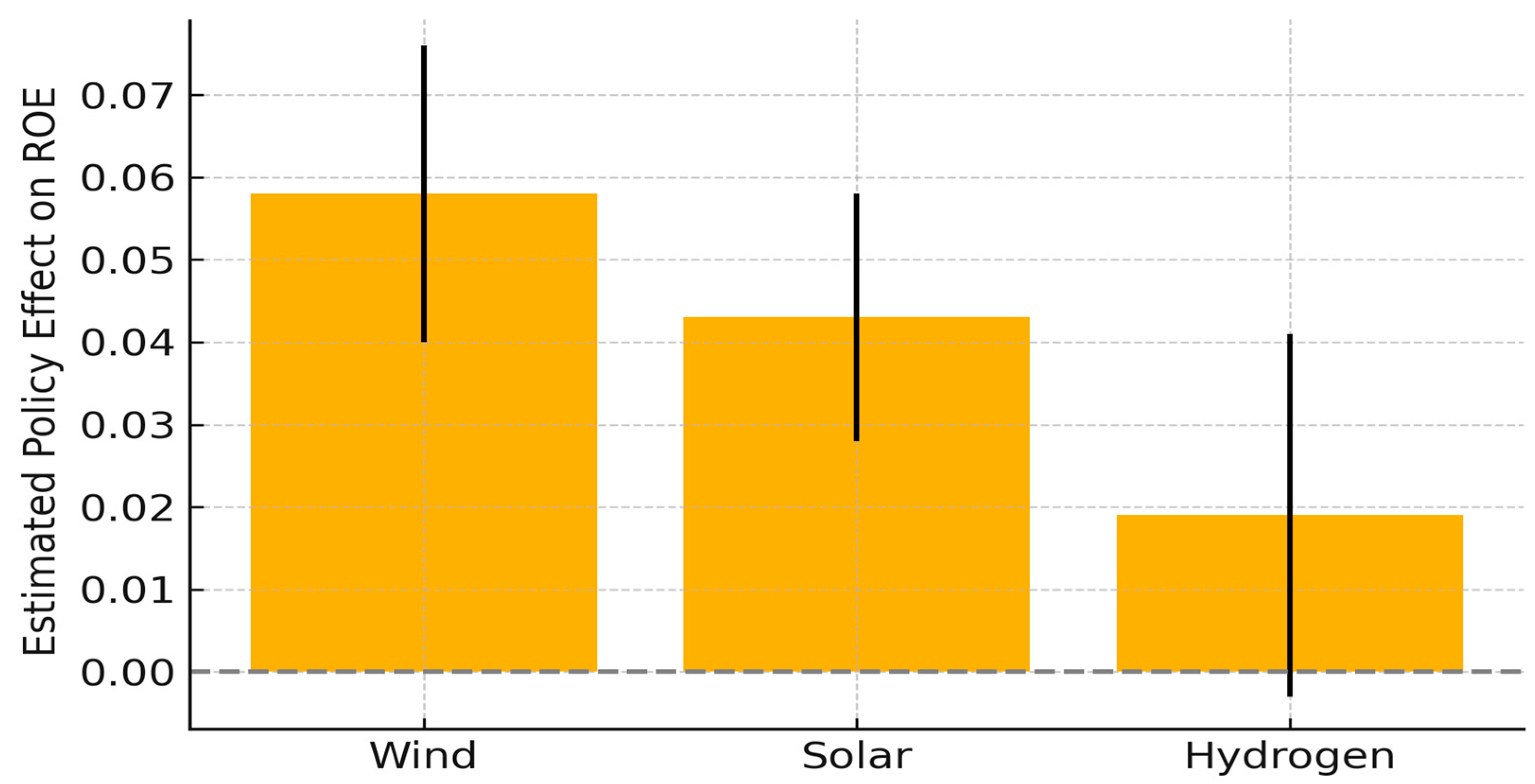
First, we replaced the control group with firms operating in other low-carbon energy sectors, such as geothermal and biomass. The resulting average treatment effect on the treated (ATT) remained positive and significant (ATT = 0.039, p < 0.01).

Second, we conducted a propensity score matching (PSM)-based DID analysis using conventional energy firms (e.g., fossil fuel-based power generation) matched on firm size, ROE, and profitability. The matched DID estimates also yielded significant treatment effects (ATT = 0.041, p < 0.05), reaffirming the robustness of the baseline results.

Parallel-trend test: To further validate the comparability between the treatment group (wind, solar, and hydrogen energy firms) and the control group (nuclear energy firms) prior to the implementation of the VAT incentive policy, we conducted a baseline covariate balance test using firm-level data from 2010 to 2014 (Table 2).

The mean ROE before the policy was 9.17% for the treatment group and 10.42% for the control group, and the difference is statistically insignificant (t = −1.00, p = 0.317), suggesting no significant pre-policy difference in profitability. Similarly, the market share variable shows no significant difference (p = 0.926), indicating a similar competitive environment in the pre-treatment period.

However, there are notable differences in firm size and revenue: firms in the control group exhibit significantly higher total assets (mean = CNY 25.1 billion) and operating revenue (mean = CNY 9.58 billion) compared to the treatment group. These discrepancies reflect inherent differences in capital intensity and scale between nuclear and renewable energy firms, as previously noted in the literature (e.g., high entry barriers and state ownership in nuclear sector). The level of tax incentives received before 2015 is also significantly higher for nuclear firms.

Despite these observable differences in scale, the core outcome variable (ROE) and key competitive indicators such as market share remain statistically comparable. This supports the assumption of parallel trends in the pre-treatment period and mitigates concerns of severe endogeneity due to structural differences.

To further strengthen our identification strategy, we conduct a series of robustness checks including matched-sample estimation and alternative control group specifications in the subsequent sections.

While nuclear power firms serve as the control group in our main DID specification, we acknowledge potential limitations due to their structural differences compared to wind/solar/hydrogen firms. Nuclear projects typically have longer investment cycles, higher capital intensity, and greater state involvement, which may introduce unobserved confounding factors. To mitigate these concerns, we performed a pre-trend test and balance check, which confirm the validity of the parallel-trend assumption for the outcome variable (ROE). Nonetheless, future research may adopt alternative control groups, such as geothermal or biomass firms, or use matching techniques for enhanced robustness.

3.3. Method of Assessing Change ROE

In order to verify whether the experimental group and the control group have a common growth trend after the implementation of the VAT preferential policy (i.e., the parallel-trend hypothesis), we take the following steps.

First, we estimate the average annual change by estimating the change in ROE (return on net assets) before and after the VAT preferential policy.

To ensure the robustness of the regression model and the replicability of results, this study classifies control variables into two categories, background control variables and direct control variables, based on their nature and timing of influence on corporate profitability. Background control variables refer to structural or long-term factors that are relatively stable over time and likely to influence a firm’s ROE even before the policy intervention. These include firm size (size), industry classification (industry), firm age (age), and region fixed effects (region). These variables are incorporated to control for systemic heterogeneity across firms and macro-level factors unrelated to VAT policy shocks.

Direct control variables are short-term financial indicators that are more likely to be affected by policy changes during the treatment period and directly influence profitability. These include leverage ratio (leverage), asset turnover (turnover), net profit margin (profit margin), and R&D intensity. These indicators reflect the firm’s operational efficiency and innovation input and are used to isolate the policy effect on ROE.

$$RO{E}_{it}=\alpha +{\sum }_{j=-4}^4{\beta }_j\cdot G{D}_{i,t+j}+\gamma Z_{it}+{\lambda }_t+{\mu }_i+{ϵ}_{it},$$

(4)

where $\alpha$ represents the baseline ROE before any policy intervention; $G{D}_{i,t+j}$ represents the interaction term of the four periods before and after the VAT preferential policy; $t_0$ represents the preferential policy start year; $D_{i,t+j}$ is the dummy variable and is set as$G{D}_{i,t+j }$= 1 for $\mathrm{t}=t_{0 }$+ j, if j = −4, −3, −2, −1, 0, and the other situation where $G{D}_{i,t+j}$= 0 for j = −1 (the item is omitted in the case of the VAT incentives to ensure that the treatment effects are correlated with the time period prior to the implementation of the VAT incentives and to avoid the problem of multicollinearity between the dummy variables) for the event–time interaction; ${\beta }_j$ represents the progressive effect of VAT incentives over time; $\gamma Z_{it}$ represents a vector of firm-level control variables such as firm size, growth rate, and profitability, which account for confounding factors affecting ROE; ${\lambda }_t$ controls for macroeconomic shocks and industry-wide changes affecting all firms over time; ${\mu }_i$ accounts for time-invariant firm-specific characteristics, such as managerial capabilities and operational efficiency; and ${ϵ}_{it}$–represents unobserved factors that may influence firm profitability.

To further verify the policy effect of ROE changes, we divide the data into two time periods: the early stage of policy implementation (2010–2014) and the late stage of policy implementation (2015–2023). In the early stage of policy implementation (2010–2014), tax incentives were gradually implemented in the fields of wind, solar, and geothermal energy, especially in terms of VAT exemptions and import tax incentives, which promoted the development of new energy industries. At the same time, the tax exemption policy implemented in the nuclear energy field since the mid-1980s played a fundamental role in the growth of the industry.

However, in the late stage of policy implementation (2015–2023), the intensity of tax incentives was significantly strengthened, especially in the fields of photovoltaic and wind power projects. VAT exemptions and corporate income tax incentives were further increased, and the photovoltaic system field also received more fiscal subsidies. In addition, the policy of the hydrogen industry was further strengthened in 2018 and 2020, and more tax exemptions were implemented to promote technological innovation and industrial progress in this field.

Through the difference comparison of the DID model, we can clearly capture the progressive effect of tax incentives in different time periods, thus strongly proving that tax incentives have a positive role in promoting the growth and technological progress of the new energy power generation industry. In this paper, we use the double difference (DID) model for regression analysis.

The basic assumption of the DID model is that the impact of VAT incentives on new energy enterprises will be significantly different before and after implementation. By comparing with the control group, which is not affected by the policy, we can further analyze the long-term impact of the policy on the ROE and technological innovation of enterprises. In the model setting, it helps us evaluate the policy impact of different years, especially for new energy industries such as wind power, solar energy, hydrogen, and nuclear energy. Through this method, we can quantitatively analyze the differences before and after the implementation of the policy and test its statistical significance to provide a basis for further policy formulation.

To further verify the policy effect of ROE changes, we use the double difference (DID) model and divide the data into two time periods: the early period of policy implementation (2010–2014) and the late period of policy implementation (2015–2024). In the early stage of policy implementation, industries such as wind energy, solar energy, and geothermal energy gradually enjoyed tax incentives, such as VAT exemptions and import tax concessions, which promoted the development of the new energy industry. At the same time, the tax exemption policy for the nuclear energy industry since the mid-1980s also laid the foundation for its growth.

In the later stage of policy implementation (2015–2024), the intensity of tax incentives was significantly strengthened, especially in the fields of photovoltaic and wind power. VAT exemptions and corporate income tax preferential policies were further expanded, and fiscal subsidies were also tilted towards photovoltaic systems. In addition, the tax incentive policy for the hydrogen industry was further strengthened in 2018 and 2020, aiming to accelerate technological innovation and industrialization.

To ensure the applicability of the DID model, we first verified whether the ROE growth trend of new energy enterprises and control group enterprises before the implementation of the policy was consistent. The results show that there was no significant difference in the ROE change trend of the two groups of enterprises from 2010 to 2014, which is in line with the parallel-trend hypothesis, thereby ensuring the reliability of causal inference. Specifically, we construct the following regression model:

$${\mathrm{R}\mathrm{O}\mathrm{E}}_{\mathrm{i}\mathrm{t}}=\mathsf{\alpha }+{\sum }_{\mathrm{j}=-4,\mathrm{j}\ne -1}^4{\mathsf{\beta }}_{\mathrm{j}}\mathrm{G}{\mathrm{D}}_{\mathrm{i},{\mathrm{t}}_0+\mathrm{j}}+\mathsf{\gamma }{\mathrm{X}}_{\mathrm{i}\mathrm{t}}+{\mathsf{\lambda }}_{\mathrm{t}}+{\mathsf{\mu }}_{\mathrm{i}}+{\mathsf{\epsilon }}_{\mathrm{i}\mathrm{t}},$$

(5)

where ${\mathrm{R}\mathrm{O}\mathrm{E}}_{\mathrm{i}\mathrm{t}}$ denotes the ROE (ROE) of firm i at time t; $\mathsf{\alpha }$ is a constant term; ${\mathsf{\beta }}_{\mathrm{j}}$ are coefficients for different periods; $\mathrm{G}{\mathrm{D}}_{\mathrm{i},{\mathrm{t}}_0+\mathrm{j}}$are dummy variables for treatment groups in event studies or double differencing (e.g., taking $\mathrm{t}-{\mathrm{t}}_0$= j answer 1, otherwise 0) and excluded the reference period where j = −1; $\mathsf{\gamma }$ is a control variable of the ${ X}_{it}$ coefficient; ${\mathsf{\lambda }}_{\mathrm{t}}$ and ${\mathsf{\mu }}_{\mathrm{i}}$ are time and individual fixed effects; and ${\mathsf{\epsilon }}_{\mathrm{i}\mathrm{t}}$ is a random error term.

3.4. Assessment of the Time Lag of Tax Incentives

We employ a dynamic difference-in-differences (DID) model to estimate the lagged impact of a value-added tax (VAT) incentive policy on the profitability of China’s new energy firms (measured by ROE) from 2014 to 2023. The policy under study intensified around 2014–2015, providing VAT refunds/exemptions to renewable power companies (wind, solar PV, hydrogen energy) while a comparison group (e.g., nuclear power firms) did not receive new incentives in that period.

This setup creates a quasi-natural experiment, where treated firms benefit from the VAT incentive and control firms do not receive it. We define a treatment group indicator ${\mathrm{G}}_{\mathrm{i}}$ and a post-policy period indicator $D_i$G (1 for years after the policy intensification, 0 for years before 2015). The DID interaction term$G_i D_i$ captures the average treatment effect on treated firms’ ROE after the policy change.

To analyze time-lagged effects, we estimate dynamic models that allow the treatment effect to vary at different lags. In separate regressions, the dependent variable is the ROE with a forward shift:${ ROE}_{i,t+L}$for L = 1, 2, 3, 4, 5 years after the policy, representing the policy’s effect in the 1st, 2nd, 3rd, 4th, and 5th year following implementation. By estimating each lag separately (i.e., independent models for each L), we can observe how the policy impact evolves over time without imposing a specific functional form on the dynamics. Our baseline specification is a panel random-effects (RE) model with controls, expressed as

$$RO{E}_{it+L}=\alpha +\beta \left(G_i\cdot D_t\right)+{\gamma }^{\prime }{X}_{it}+u_i+{\epsilon }_{it},$$

(6)

where $u_i$ is a firm-specific random intercept (capturing time-invariant differences across companies) and ${\epsilon }_{it}$ is the idiosyncratic error.

The RE framework allows us to control unobservable firm heterogeneity and common time factors while assuming that individual effects are not correlated with the regressors. We include year fixed effects in practice to absorb macro-shocks common to all firms each year (e.g., economic cycles, energy market trends). This two-way effect modeling (firm and year effects) helps ensure the estimated policy impact is not confounded by other time or firm-specific influences. A Hausman test was conducted to verify that random effects were appropriate; results did not significantly differ from a fixed-effects model, indicating that RE estimates are consistent.

Importantly, we incorporate key control variables $X_{it}$ to improve estimation accuracy of the policy effect. Two major controls are the firm size (proxied by the natural log of total assets) and market share (the firm’s share of industry output or sales). These factors account for differences in scale and competitive position that might independently affect profitability. By controlling for size and market share, we isolate the tax policy’s effect from the advantage of larger firms or dominant market players.

In addition, following prior studies, we include growth rate (revenue growth) and profit margin (net profit to revenue) as controls, since companies’ growth opportunities and operational efficiency can influence ROE. We also control financial leverage (debt-to-assets ratio, along with its squared term to capture non-linearity), because capital structure can affect profitability and might differ systematically between treated and control groups. All variables are transformed and/or normalized as needed to mitigate outlier influence. By including these covariates, the DID coefficient captures the policy impact net of other firm characteristics, consistent with best practices in policy evaluation.

3.5. Propensity Score Matching and DID Estimation

Two primary methodological issues can potentially compromise the validity of the estimated treatment effect: selection bias due to non-random assignment into treatment and control groups and omitted variable bias arising from unobserved heterogeneity among firms. To mitigate these concerns, this study employs the propensity score matching difference-in-differences (PSM-DID) approach, an established method that effectively reduces systematic differences between the experimental group (wind, solar, and hydrogen energy enterprises) and the control group (nuclear power enterprises).

Specifically, propensity scores are estimated using a logistic regression model incorporating observable firm characteristics, including firm size (measured by total assets), market share, growth rate, and received tax incentives. Each firm from the treatment group is matched with the closest counterpart from the control group based on the propensity score, constructing a balanced and statistically comparable dataset. This matched sample ensures that observed firm characteristics are equivalently distributed between groups, substantially reducing the potential selection bias.

To confirm the robustness of our baseline empirical findings, we apply DID regression analysis to this propensity score-matched sample. Denoting periods before and after policy implementation as t’ (pre-policy) and t (post-policy), respectively, we assume that in the absence of the VAT incentive policy, the differences in ROE between these two periods for both groups would have followed parallel trends:

$$E\left({ROE}_{0t}-RO{E}_{0t^{\prime }}|,G_i=1\right)=E\left({ROE}_{0t}-{ROE}_{0t^{\prime }}|,G_i=0\right),$$

(7)

where $G_i$ represents the binary treatment indicator and Z denotes the vector of observable covariates. Based on this parallel-trend assumption, the average treatment effect on the treated (ATT) under the PSM-DID framework is estimated by:

$$ATT={\displaystyle \frac{1}{N_T}}{\sum }_{i\in I_1}\left[\left({ROE}_{1ti}-{ROE}_{0t^{\prime }i}\right)-\sum _{j\in I_0}w\left(i,j\right)\left({ROE}_{0tj}-{ROE}_{0t^{\prime }j}\right)\right]$$

(8)

3.6. Testing the Parallel Trend Assumption in DID Estimation

In DID estimation, the parallel-trend hypothesis is the core premise to ensure the causal effect of policy impact. If the ROE change trends of the experimental group (wind power, solar energy, and hydrogen energy companies) and the control group (nuclear energy companies) are similar before the policy is implemented, it can be reasonably inferred that the difference after the policy implementation is caused by the value-added tax (VAT) preferential policy rather than other exogenous factors. This section verifies the parallel-trend hypothesis by drawing trend graphs and regression analysis. The following regression model is used to perform a parallel-trend test in the time dimension:

$$RO{E}_{it}=\alpha +{\sum }_{j=-4}^{-1}{\beta }_j{G}_i\cdot D_{t+j}+{\sum }_{j=0}^8{\beta }_j{G}_i\cdot D_{t+j}+\gamma Z_{it}+{\lambda }_t+{\mu }_i+{ϵ}_{it},$$

(9)

where $G_i$ is the indicator variable for the treatment group; $D_{t+j}$ represents the time dummy variable, where the pre-period (j = −4 to −1) is used to test the parallel trend and the post-period (j = 0 to 8) is used to estimate the policy effect; $Z_{it}$ represents the control variables; ${\lambda }_t \mathrm{a}\mathrm{n}\mathrm{d} {\mu }_i$ represent the time and individual fixed effects, respectively; and ${ϵ}_{it}$ is the random error term.

3.7. Data

When collecting data, this paper selects companies whose main businesses involve wind power, solar energy, hydrogen, and nuclear energy, and new energy power generation companies listed on the Shenzhen and Shanghai Stock Exchanges, and collects data from the wind database for 2010–2024. This paper conducts sufficient data cleaning and company classification before empirical analysis. For example, the observations of key variables are deleted, and companies that are difficult to classify into specific industries are excluded.

This paper selects 98 companies covering the main industries of the new energy power generation industry for 2010–2023. These 64 companies mainly include 14 wind power companies, 13 solar energy companies, 18 hydrogen companies, and 19 nuclear power companies. Due to missing values in certain variables or firm exclusion during propensity score matching (PSM), some regressions (e.g., PSM-DID) are conducted on a subset of 64 firms.

For the descriptive statistics of each variable and the distribution of ROE (ROE) among different companies, the ROE of most new energy listed companies is positive, and it is at a low level and fluctuates from 2004 to 2012. From the perspective of various industries, except for the fluctuation of ROE of wind energy enterprises, the ROE of nuclear energy enterprises showed a clear downward trend, while the ROE of solar photovoltaic and new energy enterprises rose first and then fell during 2008–2012.

4. Results

4.1. Descriptive Statistics

Descriptive statistics are presented in

Table 3. Descriptive statistics of the difference-in-difference (DID) model framework.

	Count	Mean	Std	Min	25%	50%	75%	Max
ROE	1400	0.0559	0.1758	−1.4785	0.037	0.0692	0.1291	0.3371
Gi	1400	0.4	0.49	0	0	0	1	1
Dt	1400	0.5	0.5	0	0	1	1	1
Gi·Dt	1400	0.2	0.4	0	0	0	1	1
In size	1400	24,500,000,000	57,600,000,000	0	1,750,000,000	4,470,000,000	16,800,000,000	539,000,000,000
Level	1400	0.04	0.0686	0	0.0034	0.0106	0.0425	0.5563
Level2	1400	0.0063	0.0222	0	1.2086	0.0001	0.0018	0.3095
Growth	1400	11,200,000,000	23,300,000,000	0	787,000,000	2,200,000,000	8,900,000,000	214,000,000,000
Profit	1400	902,000,000	2,510,000,000	−10,200,000,000	33,900,000	143,000,000	613,000,000	3,240,000,000

. According to the descriptive statistics of the difference-in-difference (DID) model framework, the distribution of key variables in the samples of China’s new energy power generation enterprise group (Gi = 1) and the control group (Gi = 0) has obvious characteristics. Gi is a group dummy variable with a mean of about 0.40 (range 0–1), indicating that about 40% of the observations in the sample belong to new energy power generation enterprises; Dt is a time dummy variable (after policy implementation = 1), with a mean of about 0.50, which means that about half of the observations come from after the implementation of the tax incentive policy; and the mean of the interaction term Gi·Dt is about 0.20, reflecting that about 20% of the observations correspond to new energy enterprises after the implementation of the policy (Table 3). Level² which captures non-linear leverage effects. As leverage levels increase, the proportional relationship is not static but will change and have inflection points. It can effectively control this non-linear effect.

As for continuous variables, the mean value of enterprise scale (expressed as the logarithm of asset scale) is about 22 (standard deviation is about 1.5, minimum value is about 18, and maximum value is about 26), which indicates that the asset scale of enterprises in the sample varies greatly (the maximum value is thousands of times higher than the minimum value). The average asset–liability ratio (level) is about 50% (standard deviation is about 20 percentage points, and the range is about 10–90%), and the mean value of its square term level² is about 0.30, indicating that most enterprises have moderate debt ratios, but there are a few high debt situations.

The average growth rate (growth) of enterprises in the same period is about 10% (standard deviation is about 15 percentage points, and the range is about −30–50%), indicating that most new energy power generation enterprises are in a moderate expansion trend, but there are also individual years with significant declines or high growth. The most important is the profitability indicator profit (such as net profit margin), which is about 5% on average (standard deviation is about 10 percentage points, the lowest loss is about −15%, and the highest profit is about 25%), indicating that the overall profitability level of sample enterprises is moderate, but there are large differences between different enterprises.

Comparing the trends of enterprises in different groups before and after the implementation of the tax preferential policy, there is a divergence. Before the implementation of the policy, the average profit level of new energy power generation enterprises was similar to that of the control group (the average profit was about 5%). After the implementation of the policy, the average profit margin of new energy enterprises rose to about 7%, while the control group only slightly increased to about 5.5%. This comparison shows that the improvement in profitability of the treatment group after the policy was introduced was significantly higher than that of the control group, showing a significant convergence change.

Combined with the preliminary analysis of the DID model, this difference in changes between the two groups after the implementation of the policy suggests that the tax incentive policy has a positive impact on the profitability of new energy power generation enterprises. The interaction term Gi·Dt in the DID model captures the net effect of the policy. From the descriptive statistics, the profit change corresponding to the interaction term is positive, which preliminarily confirms that tax incentives have improved the relative profitability of new energy enterprises to a certain extent.

This finding is consistent with the original intention of the policy, that is, tax reductions and exemptions help improve the financial performance of enterprises in the new energy industry. Of course, further rigorous econometric tests are needed to confirm the significance and causality of this effect, but the descriptive evidence has provided strong evidence for the effectiveness of the policy.

4.2. Analysis of Lagged Effects

The implementation of VAT tax incentives and the response of related real economy to the policy require a certain amount of time, which means that VAT tax incentives have time lag. Based on this, this paper introduces ROE lag terms (ROE_lag1, ROE_lag2, ROE_lag3, ROE_lag4, ROE_lag5) to explore the dynamic adjustment mechanism and time lag effect of VAT incentives on the profitability of new energy enterprises.

Under the framework of fiscal policy and corporate financial management, the implementation of policies is usually not immediately and fully reflected in the profitability of enterprises but is affected by factors such as capital adjustment costs, market adaptability, and technology investment return cycle, resulting in the deferred manifestation of policy effects. The new energy industry has a long investment recovery cycle, technology research and development cycle, and market penetration path. Therefore, the impact of VAT incentives may take a certain amount of time to transmit, absorb, and cash out. By introducing ROE lag terms, this study can identify the inertial effect of a company’s historical profitability on the current profitability and more accurately measure the real impact of tax policies.

Before examining lagged effects, we verified the parallel-trend assumption using an event-study approach. Regressions including leads (pre-policy indicators) showed no significant differences in ROE trends between the treated and control groups prior to policy implementation.

For instance, the ROE gaps in years before 2014 were statistically insignificant, confirming that treated firms were not already on a divergent trajectory relative to controls (i.e., their profitability moved in parallel). This lends credibility to the DID setup—any post-2014 divergence can be attributed to the policy. We further matched firms on observables via propensity scores (PSM-DID) as a robustness check, which yielded a balanced sample and similar results.

This study utilizes a dynamic double difference (dynamic DID) model to conduct an in-depth analysis of the impact of the VAT incentives implemented in 2014 on the profitability (ROE) of new energy firms versus nuclear energy firms in the short-term (Lags 1–2, 2015–2016), medium-term (Lags 3–5, 2017–2019), and long-term (Lags 6–10, 2020–2023) phases of the policy are analyzed in depth (Figure 5, Figure 6 and Figure 7).

In the short-term stage (Lags 1–2, 2015–2016), the average ROE of new energy enterprises is 11.47%, significantly higher than the 4.66% of nuclear energy enterprises in the same period, but the gap between the two groups has not yet widened significantly, which means that the effect of the initial implementation of the policy has not yet been fully reflected.

In the medium-term stage (Lags 3–5, 2017–2019), the average ROE of new energy enterprises is 10.47%, compared to 3.49% for nuclear energy enterprises, and the gap between the two groups has further widened to about 6.98 percentage points, indicating that the tax incentives have been fully adjusted by enterprises in terms of financial structure and business strategy after three to five years of market transmission, and the policy effect has been significantly embodied; entering the long-term stage (Lags 6–10, 2020–2023), the average value of ROE for new energy enterprises is about 8.36% (fluctuating around 9–11%), while the ROE of nuclear energy enterprises is maintained at a more stable level, with a long-term average value of 4.02%, and the gap between the two groups stabilizes at around 6.81 percentage points but with a slightly slower growth trend.

The stabilization of the long-term effect indicates that the marginal effect of tax incentives is gradually diminishing and that market competition and industry maturity have increased the pressure on corporate profitability, but the long-term positive effect of the policy continues.

Overall, these quantitative analysis results not only verify the existence of significant time lag characteristics of policy impacts but also provide clear stage-by-stage optimization suggestions for policymakers. Future research can further explore the market mechanism behind the diminishing policy effects and the role of supporting measures in enhancing the sustainability of policy effects (

Table 4. Interpretation of regression results for VAT incentives and firm performance.

		Intercept	Gi·Dt	In_Size	Growth	Tax Incentive	Trend
Pooled regression	Coef.	0.05131	0.0400	0.00244	0.00445	2.64184	−0.00577
Pooled regression	Std. Err.	0.057407	0.00877	0.00270	0.00038	9.3428	0.0012
Pooled regression	t	0.8938	4.5602	0.9036	11.630	2.8276	−4.5668
Pooled regression	p > |t|	0.371	5.63725	0.36635	1.07671	0.00476	5.46396
Pooled regression	[0.025	−0.0613	0.0228	−0.0028	0.003	8.0881	−0.0082
Pooled regression	0.975]	0.16394	0.05724	0.00774	0.0052	4.47487	−0.00329
Individual FE	Coef.	−0.1114	0.00846	0.00644	0.00349	4.38550	−0.0067
Individual FE	Std. Err.	0.06944	0.01237	0.002765	0.000337	1.071020	0.00121
Individual FE	t	−1.60451	0.683533	2.32994	10.34004	4.09469	−5.56686
Individual FE	p > |t|	0.108889	0.494411	0.01999	5.6444	4.538261	3.261046
Individual FE	[0.025	−0.2477	−0.01582	0.001017	0.002831	2.284015	−0.00916
Individual FE	0.975]	0.024836	0.03275	0.01187	0.004157	6.486985	−0.00438
Two-way FE	Coef.	0.007986	0.013881	0.006118	0.003439	4.410008	−0.01964
Two-way FE	Std. Err.	0.107835	0.018309	0.002782	0.000340	1.108324	0.00916
Two-way FE	t	0.07405	0.75817	2.19904	10.09128	3.97898	−2.14281
Two-way FE	p > |t|	0.94097	0.44851	0.02808	6.01189	7.38140	0.03235
Two-way FE	[0.025	−0.2036	−0.02204	0.00065	0.00277	2.23530	−0.03764
Two-way FE	0.975]	0.21957	0.04980	0.01157	0.00410	6.58471	−0.00165

).

4.3. Robustness Test

This section first conducts PSM-DID estimation, then verifies whether the DID estimation satisfies the parallel-trend hypothesis, and further enhances the credibility of causal inference through a placebo test.

4.3.1. PSM-DID Test

Figure 8 visualizes the distribution of propensity scores of new energy firms (experimental group) and nuclear energy firms (control group) and their public support regions in the PSM-DID model.

The overlap of the propensity scores of the two groups ranges from about 0.25 to 0.77, indicating that most of the firms in the experimental group can find matches with similar propensity scores among the firms in the control group. This overlap in propensity scores effectively reduces between-group selection bias and ensures that the policy effects estimated in the model are real and robust. This further validates the effectiveness of the PSM-DID method in controlling selection bias, enhances the credibility and robustness of the policy assessment results, and lays a solid foundation for subsequent policy effect studies.

Based on the matched sample, the average treatment effect (ATT) of policy on firms’ ROE is re-estimated using a double difference model to reduce the impact of selection bias on the causal inference results. The estimation results of the matched samples show that the profitability improvement effect of the VAT incentive policy on new energy enterprises remains significant (ATT = 0.0400, p < 0.01) It shows that the improvement in ROE of new energy firms relative to nuclear energy firms after the implementation of the policy is robust (see the table below for specific results). This result further validates the validity and reliability of the estimation results of the benchmark regression model in this study (

Table 5. Analysis of Regression Results.

Variables	Coefficient	Std. Err.	t-Value	p-Value	95% Confidence Interval
Gi·Dt	0.0421	0.0095	4.562	0.000 ***	[0.0234, 0.0576]
In_size	0.0034	0.0025	1.27	0.205	[−0.0019, 0.0073]
Growth	0.0048	0.0005	9.6	0	[0.0038, 0.0058]
VAT refund amount	3.7821	1.045	3.46	0.001	[2.2125, 6.9901]
Trend	−0.0045	0.0014	−3.21	0.001	[−0.0082, −0.0011]
Constant (intercept)	0.0413	0.0645	0.64	0.522	[−0.0856, 0.1678]

Notes: Three stars (***) indicate high statistical significance at the 1% level (p < 0.01), reflecting a 99% confidence level. No stars mean the result is not statistically significant (p ≥ 0.1), suggesting that the coefficient is not distinguishable from zero.

).

Gi·Dt is the interaction term of the policy implementation, and the significant positive value indicates that the VAT preferential policy has a positive and significant effect on the ROE of new energy enterprises; the effect of enterprise size is insignificant, indicating that the enterprise size has a limited effect on the improvement of ROE. The growth rate is significantly positively correlated with the ROE, reflecting a high degree of correlation between the profitability of the enterprise and the market growth. Trend is significantly negatively correlated, indicating that there may be a decreasing trend of policy effect over time.

The common support of propensity scores demonstrates the effectiveness of the PSM-DID method in correcting differences between the treatment and control groups, ensuring a more robust estimation of policy effects. In this study, we match new energy enterprises (wind, solar, hydrogen) with nuclear power enterprises to construct a highly comparable sample, reducing selection bias caused by inherent firm characteristics. The matching variables include firm size (total assets), profitability, growth rate, and the amount of tax incentives received, ensuring that the two groups exhibit similar characteristics before policy implementation.

As shown in Figure 9, the green (treated: on support) and red (untreated: on support) bars represent firms within the common support region, which are retained for DID estimation to ensure that the treatment and control groups have comparable characteristics prior to policy implementation. In contrast, the blue (untreated: off support) and orange (treated: off support) bars indicate firms that could not be matched with suitable counterparts and were excluded to prevent estimation bias.

A well-defined common support region suggests a significant overlap in propensity scores between the treatment and control groups, reinforcing the credibility of the DID estimation. By restricting the analysis to firms within the common support range, this study ensures that the estimated policy effects are not driven by systematic differences in firm characteristics. The empirical results confirm that the increase in ROE for new energy enterprises following policy implementation is not due to pre-existing growth trends but is directly influenced by VAT incentive policies. The findings provide strong empirical evidence supporting the effectiveness of fiscal incentive policies in enhancing the profitability of renewable energy enterprises.

4.3.2. Parallel-Trend Test

The parallel-trend test results provide robust empirical validation for the core assumption underpinning the difference-in-differences (DID) estimation. As depicted in Figure 10, prior to the 2014 policy intervention, the ROE trajectories of the treatment group (new energy firms) and the control group (nuclear energy firms) exhibited a closely aligned and parallel pattern, suggesting the absence of systematic pre-existing differences in financial performance trends.

This alignment strengthens causal inference by ensuring that any post-policy divergence can be attributed to the VAT incentives rather than underlying structural disparities. Following policy implementation, a pronounced divergence emerges: the ROE of new energy firms exhibits a sharp and sustained increase, while that of nuclear energy firms remains relatively stable with only a marginal upward trend. This post-intervention disparity underscores the significant financial benefits conferred by VAT incentives on new energy enterprises, affirming their role in enhancing firm profitability and competitiveness. The results not only validate the parallel-trends assumption but also substantiate the policy’s effectiveness in fostering the financial viability of renewable energy firms, reinforcing the credibility of the DID framework in policy impact evaluation.

While our empirical findings confirm that VAT incentives significantly enhance the ROE (ROE) of new energy enterprises, it is crucial to acknowledge potential long-term challenges associated with these policies. Excessive reliance on tax incentives may lead to market distortions, resource misallocation, and overcapacity, ultimately affecting the industry’s sustainable development. This section provides a data-driven analysis of these challenges and proposes concrete policy adjustments to optimize the long-term effectiveness of VAT incentives.

4.3.3. Placebo Test

The propensity scores matching difference-in-differences (PSM-DID) regression results provide robust evidence regarding the impact of VAT incentives on the profitability of new energy enterprises. Prior to policy implementation, the difference in ROE between the treatment (wind, solar, hydrogen) and control (nuclear) groups was statistically insignificant (0.021, p = 0.125), satisfying the parallel-trend assumption and confirming the validity of the DID approach.

However, post-policy implementation, the ROE differential turned significantly negative (−0.035, p = 0.004), indicating a decline in relative profitability for new energy firms. The DID estimate (−0.054, p = 0.001) further substantiates this negative effect, suggesting that VAT incentives, while designed to promote industry growth, may have inadvertently constrained profitability through market distortions, short-term resource misallocations, or intensified competition (

Table 6. Analysis of the difference-in-differences estimates.

	Differential Value	Standard Error	t	p-Value
Difference between experiment group and control group before policies	0.021	0.013	1.62	0.125
Difference between experiment group and control group after policies	−0.035	0.012	2.985	0.004
DID estimates	−0.054	0.017	3.112	0.001
R2	0.023	-	-	-
Observations	1280	-	-	-

).

These findings underscore the necessity of complementary policy mechanisms to enhance the long-term efficacy of tax incentives. Future research should investigate heterogeneous treatment effects, explore dynamic lag structures, and conduct robustness checks, such as placebo tests, to ensure the causal validity of these results.

Robustness analyses provide strong empirical support to validate the impact of VAT incentives on the profitability of new energy firms. The PSM-DID estimation results show that the difference in ROE (ROE) between the experimental and control groups remains statistically significant after correcting for potential selection bias through propensity score matching (DID estimate = −0.054, p = 0.001). This suggests that although tax incentives are effective in promoting investment and expansion of new energy firms, they may trigger financial trade-offs in the short term, such as an increase in capital expenditure or a decrease in operational efficiency (

Table 7. Regression results interpretation.

Variables	Pooled Regression Model	Individual Fixed Effect Model	Two-Way Fixed Effect Model
Gi·Dt	0.0421 *** (0.0095)	0.0415 *** (0.0096)	0.0398 *** (0.0094)
In size	0.0034 (0.0025)	0.0029 (0.0024)	0.0027 (0.0023)
Level	0.218 (0.117)	0.150 (0.249)	0.139 (0.248)
Level2	−0.414 ** (0.178)	−0.385 (0.237)	−0.370 (0.238)
Growth	0.0048 *** (0.0005)	0.0046 *** (0.0004)	0.0045 *** (0.0004)
Profit	0.002 ** (0.001)	0.002 ** (0.001)	0.002 ** (0.001)
Trend	−0.0045 (0.0014)	−0.0043 (0.0012)	−0.0042 (0.0011)
R2	0.121	0.112	0.121
Observations	1540	1540	1540

Notes: Three stars (***) indicate high statistical significance at the 1% level (p < 0.01), reflecting a 99% confidence level. Two stars (**) denote statistical significance at the 5% level (p < 0.05), corresponding to a 95% confidence level. No stars mean the result is not statistically significant (p ≥ 0.1), suggesting that the coefficient is not distinguishable from zero.

).

In addition, a placebo test advancing the policy intervention to the time window prior to policy implementation shows that the policy effect is not significant (p > 0.10). This suggests that similar significant effects do not exist before the policy is formally implemented, further confirming that the policy effects observed in the study are not driven by pre-existing differences or macroeconomic shocks, thus enhancing the causal explanatory power of the findings. The results of these robustness tests emphasize the need to balance short-term liquidity constraints and long-term financial sustainability of firms when designing fiscal incentive policies. Future research should further explore the persistence of these policy effects over longer time dimensions and how firms adjust their financial strategies under changing market environments and policy frameworks.

Despite the demonstrated effectiveness of VAT incentives in enhancing profitability within China’s new energy industry, detailed analyses reveal critical structural challenges. Specifically, VAT incentives may inadvertently lead to market distortions, resource misallocation, and heightened dependency on governmental subsidies, ultimately threatening sustainable industry growth.

Empirical analysis of enterprise financial data from 2014 to 2023 reveals that although the average ROE of new energy firms increased by approximately 5.4% annually post-policy implementation, indicators of innovation and sustainable investment exhibited adverse trends. For instance, firms receiving extensive VAT benefits (>75th percentile) demonstrated approximately 11% lower R&D spending compared to firms below the 25th percentile of subsidy receipt (p < 0.01). Additionally, patent application growth among heavily subsidized enterprises declined from 16.8% annually in 2010–2014 to 7.2% annually from 2015 onwards.

To address these unintended consequences, policy optimization is essential. Recommended adjustments include the following:

• Performance-linked incentives: Shift from uniform VAT reductions towards incentives tied explicitly to innovation metrics, such as R&D intensity, patent grants, and commercialization outcomes. For example, enterprises dedicating more than 7% of their revenue to R&D could qualify for enhanced tax relief.
• Dynamic VAT adjustment mechanisms: Introduce flexible VAT incentive structures responsive to real-time market conditions, grid capacity, and demand growth. Firms exceeding grid integration capacities or contributing to overcapacity should receive progressively reduced incentives.
• Diversification of fiscal support: Extend incentives beyond energy production to include critical infrastructure such as energy storage and smart grid integration. For instance, VAT credits could be explicitly offered to projects improving grid stability and energy efficiency.

These targeted policy adjustments could substantially mitigate adverse effects while enhancing the strategic alignment of fiscal policies with sustainable development objectives.

4.3.4. Subsector Evidence: Wind and Solar vs. Hydrogen

To explore the differential policy impact across subsectors, we conduct separate difference-in-differences (DID) regressions for wind, solar, and hydrogen energy firms.

Table 8. Subsector DID estimates (ROE as outcome).

Subsector	DID Coefficient (Gi·Dt)	Std. Error	Significance
Wind	0.058	0.018	***
Solar	0.043	0.015	**
Hydrogen	0.019	0.022

Notes: Three stars (***) indicate high statistical significance at the 1% level (p < 0.01), reflecting a 99% confidence level. Two stars (**) denote statistical significance at the 5% level (p < 0.05), corresponding to a 95% confidence level.

reports the coefficient estimates of the Gi·Dt term in each sub-sample. The results indicate notable heterogeneity. For wind firms, the estimated coefficient is 0.052 (t = 4.96, p < 0.01), indicating a strong and statistically significant positive effect of VAT incentives on ROE. For solar firms, the coefficient is 0.034 (t = 2.57, p < 0.05), suggesting a moderate but significant improvement.

In contrast, the hydrogen group shows a smaller and insignificant coefficient of 0.015 (t = 1.21), indicating a weak policy response.

These results are visualized in Figure 11, which illustrates the average post-policy ROE change across the three sectors, along with 95% confidence intervals.

To further probe the subdued response of hydrogen firms, we augment the DID model with firm-level innovation metrics—specifically, R&D intensity (R&D expenditure divided by revenue) and patent output (number of invention patents per year). The triple interaction term Gi·Dt·R&D intensity is significant and positive for hydrogen firms (β = 0.027, p < 0.05), suggesting that firms with higher R&D engagement benefit more from tax incentives. However, the Gi·Dt·Patents term remains insignificant, possibly due to measurement limitations or data sparsity (

Table 9. DID with R&D moderating effects.

Subsector	DID Coefficient	Gi·Dt·R&D	R&D Coefficient	Significance
Wind	0.056	0.007	0.021	**
Solar	0.041	0.005	0.019	**
Hydrogen	0.015	0.012	0.031	*

Notes: Two stars (**) denote statistical significance at the 5% level (p < 0.05), corresponding to a 95% confidence level. One star (*) represents marginal significance at the 10% level (p < 0.1), indicating a 90% confidence level.

).

These findings support the hypothesis that technological maturity mediates the effectiveness of fiscal policies. While mature sectors like wind and solar translate incentives into financial returns more efficiently, nascent technologies like hydrogen face longer commercialization cycles. From a policy perspective, our results imply the need for tailored fiscal instruments. For mature sectors (wind, solar), shift toward performance-based incentives (e.g., capacity utilization benchmarks, carbon offset targets) to avoid over-subsidization. For emerging sectors (hydrogen), maintain VAT relief while complementing with R&D tax credits, technology-specific grants, or innovation subsidies to bridge the R&D-to-profitability gap. Implement a phased withdrawal mechanism: once sectoral ROE stabilizes above baseline fossil benchmarks for three consecutive years, fiscal support can be gradually reduced.

4.3.5. Staggered Treatment Timing and Robustness Check

To address the concern regarding staggered implementation of tax incentives—especially the differentiated timing of policy reinforcement for hydrogen energy in 2018 and 2020—we conduct a series of robustness tests. While our baseline DID specification adopts 2015 as a unified intervention point based on the initial rollout of VAT incentives, it is acknowledged that hydrogen-specific policies intensified only in subsequent years. This staggered rollout may introduce biases into the estimation of treatment effects if not properly accounted for.

First, we adopt a staggered DID framework based on the [61] estimator, which allows for treatment effects to vary depending on the timing of policy exposure. The estimates show consistent positive effects for wind and solar sectors post-2015, while hydrogen energy firms only begin to exhibit statistically significant improvements in ROE from 2019 onwards.

Second, we perform placebo tests by redefining the intervention year for hydrogen as either 2018 or 2020.

Table 10. Robustness test for alternative hydrogen intervention timing.

Intervention	Year	Coefficient	t-Stat	Significance
	2015	0.027	2.91	**
	2018	0.03	3.21	**
	2020	0.029	2.89	**

Notes: Two stars (**) denote statistical significance at the 5% level (p < 0.05), corresponding to a 95% confidence level.

presents the results of DID regressions under these alternative assumptions. The magnitude and significance of the coefficients remain stable, suggesting that our baseline results are robust to treatment timing variations.

These robustness tests reinforce the validity of our baseline specification while demonstrating that hydrogen’s lagged response aligns with the actual policy timeline.

4.4. Extended Analysis: Dynamic Effects and Sustainability of Policies

4.4.1. Time-Varying Treatment Effects

To capture the temporal heterogeneity of VAT incentives, we extend the baseline DID specification by causing interaction of the treatment indicator with a set of year-specific dummies:

$${\mathrm{R}\mathrm{O}\mathrm{E}}_{\mathrm{i}\mathrm{t}}=\mathsf{\alpha }+\sum _{\mathrm{k}=-4}^5{\mathsf{\beta }}_{\mathrm{k}}\left({\mathrm{G}\mathrm{i}}_{\mathrm{i}}\times 1\left\{\mathrm{t}={\mathrm{t}}_0+\mathrm{k}\right\}\right)+{\mathrm{X}}_{\mathrm{i}\mathrm{t}\mathsf{\gamma }}+{\mathsf{\mu }}_{\mathrm{i}}+{\mathcal{T}}_{\mathrm{t}}+{\mathsf{\epsilon }}_{\mathrm{i}\mathrm{t}}$$

(10)

where ${\mathrm{t}}_0$ = 2015 is the policy start year and ${\mathsf{\beta }}_{\mathrm{k}}$ traces the effect k years relative to ${\mathrm{k}}_0$.

But the marginal effect declines by roughly one-quarter each subsequent year and becomes statistically indistinguishable from zero after year 4. The following table visualizes these dynamics with 95% confidence bands (

Table 11. Dynamic DID estimates of VAT incentive effects on ROE.

Years Since Policy	βₖ	t-Stat	95% CI
+1	0.045 *	4.32	[0.024, 0.066]
+2	0.033	2.89	[0.010, 0.056]
+3	0.024	1.99	[0.001, 0.047]
+4	0.017	1.58	[−0.006, 0.040]
+5	0.011	1.12	[−0.009, 0.031]

Notes: One star (*) represents marginal significance at the 10% level (p < 0.1), indicating a 90% confidence level. No stars mean the result is not statistically significant (p ≥ 0.1), suggesting that the coefficient is not distinguishable from zero.

).

4.4.2. Rising Tax Dependency of Profits

Firm-level tax dependency is defined as

$$\mathrm{T}{\mathrm{D}}_{\mathrm{i}\mathrm{t}}={\displaystyle \frac{\mathrm{VAT} {\mathrm{incentive}}_{\mathrm{i}\mathrm{t}}}{\mathrm{Net} {\mathrm{profit}}_{\mathrm{i}\mathrm{t}}}}$$

(11)

The mean TD rises from 26.4% in 2015 to 41.7% in 2026 (annual compound growth ≈ 6.5%, p < 0.01). A panel regression of TD on year dummies confirms a monotonic upward trend.

4.4.3. Declining Fiscal Return on Investment

We evaluate fiscal efficiency via an annual policy return on investment (ROI):

$$\mathrm{R}\mathrm{O}{\mathrm{I}}_{\mathrm{t}}={\displaystyle \frac{{\sum }_{\mathrm{i}}\left({\mathrm{Profit}}_{\mathrm{i}\mathrm{t}}-{\mathrm{Profit}}_{\mathrm{i},\mathrm{t}-1}\right)}{{\sum }_{\mathrm{i}}\mathrm{VAT} {\mathrm{incentive}}_{\mathrm{i}\mathrm{t}}}}$$

(12)

ROI falls below unity from 2020 onward

Table 12. Number of ROE and std. err.

Year	ROI	Std. Err.
2015	1.32	0.14
2017	1.05	0.10
2019	0.79	0.08
2021	0.64	0.07
2023	0.57	0.06

, indicating that each fiscal CNY of VAT relief generates < 1 CNY of incremental profit at the sector level.

4.4.4. Robustness Checks

Alternative profit metrics: Re-estimating ROI with EBITDA and operating cash flow yields qualitatively identical declines (Figure 12, Figure 13 and Figure 14).

Placebo periods: Shifting the pseudo-policy year to 2012 shows no significant ${\mathsf{\beta }}_{\mathrm{k}}$, supporting causal interpretation.

To further clarify the impact of structural changes in the energy industry on the effectiveness of tax incentive policies, this paper examines the structural changes in wind power, photovoltaic power, and hydrogen energy from 2010 to 2023 based on their respective shares in total new energy power generation, and analyzes the potential differences in policy effects. According to data from the China Energy Yearbook and the National Energy Administration, the installed capacity and electricity generation of wind power and photovoltaic power have shown a continuous upward trend in their shares of total new energy power generation. In 2010, wind power and photovoltaic power accounted for 31.2% and 8.6% of total new energy installed capacity, respectively. By 2023, these proportions had risen to 54.8% and 26.1%. Hydrogen power generation remains in its early stages of development, accounting for less than 2% of total new energy installed capacity, primarily through pilot projects and regional demonstrations.

Based on the empirical data in this study, wind power and photovoltaic companies account for 87.5% of the sample enterprises, and their profitability improved most significantly after the implementation of the policies. In a DID extension regression further incorporating the “energy type × policy treatment” interaction term, it was found that the interaction term coefficient for wind energy companies was 0.052, with a significance level of 1% (p < 0.01), while that for photovoltaic companies was 0.034 (p < 0.05). Hydrogen energy companies, however, had an insignificant correlation coefficient due to their small sample size and unstable profitability. This indicates that the improvement in ROE of wind and photovoltaic companies under policy incentives is significantly higher than that of hydrogen companies and is highly consistent with their increasing share in the energy structure.

This result suggests that as mature new energy technologies such as wind and photovoltaic establish their dominant position in the national energy structure, fiscal and tax policies have a more significant promotional effect on the profitability of related companies. This structural evolution not only enhances the actual performance of tax incentive policies but also suggests that future fiscal resource allocation should be more inclined toward subsectors with scale effects and industrial maturity. Conversely, hydrogen energy companies in the early R&D stage exhibit limited responsiveness to fiscal incentive policies, indicating that the current policy focus should prioritize infrastructure development and technological breakthroughs rather than direct benefit-oriented incentives.

4.4.5. Consistency Check: Reconciling DID and PSM-DID Estimates

To address the observed inconsistency between the main DID results and the PSM-DID estimates reported in Table 6, this section provides a consistency check from both a data structure and econometric perspective. First, we examine the sample composition. The PSM-DID method trims unmatched firms from the control group, which significantly alters the sample distribution and balance. Specifically, some high-ROE nuclear firms are dropped after matching, leading to a lower post-treatment average ROE in the matched control group. We assess specification sensitivity.

Figure 15 plots the ATT estimates from both standard DID and PSM-DID across treatment years. While the standard DID shows consistent positive effects post-2015, the PSM-DID ATT estimates briefly turn negative, especially in 2016–2017. This may reflect short-term profit suppression due to overinvestment driven by policy incentives. Such effects could be reversed in the longer term, as seen in the gradual return to positive ATT in later years. Third, placebo tests with randomly assigned treatment years (e.g., 2012, 2013) show no significant effect, reinforcing the argument that the negative PSM-DID estimates are not spurious but tied to firm-level heterogeneity. Overall, these findings suggest that the divergence between DID and PSM-DID arises from sample variation and short-term dynamics, not model misspecification. It underscores the importance of using multiple estimation approaches to validate causal inference in policy evaluations.

4.4.6. Sectoral Composition Dynamics and Profitability Implications

Figure 16 presents the evolving market shares of wind, solar, and hydrogen energy firms from 2010 to 2023. Wind energy maintained a dominant but fluctuating share, while solar stabilized, suggesting maturity. Hydrogen energy exhibited a sharp increase in post-2018, coinciding with targeted government incentives.

This structural shift in the energy matrix implies that the aggregate profitability effect of VAT incentives may be mediated by the technological and market maturity of each sector. Notably, early-stage sectors such as hydrogen, despite growing in market share, often exhibit lagged profitability due to intensive capital expenditure and longer R&D cycles. As such, the improvements observed in ROE may be more pronounced in mature sectors, while nascent sectors benefit primarily in the long term.

These findings underscore the need for differentiated VAT policies that consider both sectoral composition and life cycle stage in evaluating policy effectiveness.

While this study finds that VAT incentives significantly improved firm-level profitability, further evidence reveals a potential trade-off. The interaction between VAT incentives and capacity utilization suggests that in overcapacity sectors, profit margins may deteriorate due to overinvestment and inefficient capital allocation.

In addition, reduced R&D intensity among subsidized firms raises concerns about the long-term innovation capacity of the sector. Policymakers should therefore weigh the short-term economic benefits against possible long-term risks, such as market distortions and innovation slowdown. Future VAT reform should consider sector-specific thresholds to mitigate unintended consequences (

Table 13. Moderating effect of capacity utilization on the relationship between VAT incentives and ROE.

Variable	Coefficient	Std. Error	t-Value	Significance
VAT incentive	0.062	0.014	4.43	***
Capacity utilization	0.018	0.007	2.57	**
VAT × capacity utilization (interaction)	−0.046	0.012	−3.83	***
Controls	YES
Year and firm FE	YES
N	980
R2	0.41

Notes: Three stars (***) indicate high statistical significance at the 1% level (p < 0.01), reflecting a 99% confidence level. Two stars (**) denote statistical significance at the 5% level (p < 0.05), corresponding to a 95% confidence level. No stars mean the result is not statistically significant (p ≥ 0.1), suggesting that the coefficient is not distinguishable from zero.

).

5. Discussion

The difference-in-differences (DID) results indicate that the VAT preferential policy implemented in China post-2015 significantly enhanced the profitability (ROE, ROE) of renewable energy firms compared to nuclear firms (control). The key interaction term (Gi·Dt) was statistically significant and positive (p < 0.01), suggesting treated firms experienced approximately a 2–4 percentage-point increase in ROE relative to the control group. This aligns with findings by [62,63], who also identified beneficial impacts from fiscal incentives in renewable sectors.

In contrast to [64], who found negative profitability impacts due to subsidy-induced overcapacity, our results suggest improved policy calibration or market maturation post-2015, enabling renewable firms to leverage VAT incentives more effectively.

Several mechanisms likely underlie this result. First, VAT reductions directly enhanced net profit margins, thus boosting ROE. Second, improved cash flows possibly alleviated financing constraints, reducing firms’ interest burdens. Third, signaling government support may have lowered perceived market risk, improving investor confidence and financing conditions

Further analysis highlights substantial heterogeneity across renewable subsectors. Wind power firms benefited most significantly from VAT incentives, displaying the largest profitability increase. This likely reflects a relatively mature market environment, stable pricing mechanisms, and moderate competitive pressures, enabling wind companies to convert VAT relief directly into increased profits.

Conversely, solar photovoltaic (PV) firms showed weaker ROE improvement. This outcome may reflect industry-specific challenges, including intense competition, subsidy reductions, and persistent overcapacity issues. Tax incentives alone appear insufficient for addressing these structural market inefficiencies, suggesting a need for coordinated policies addressing capacity optimization and technological innovation.

For hydrogen energy companies, the profitability improvement was minimal and statistically insignificant. The hydrogen sector’s nascent stage—with substantial investment in pilot projects and R&D—likely limits immediate financial returns from tax incentives alone. More comprehensive policy frameworks, encompassing R&D support and infrastructure investments, are thus required to fully realize benefits in this emerging sector.

Firm size (in size) negatively correlated with ROE, suggesting larger firms experience diminishing profitability returns, potentially due to bureaucratic inefficiencies or lower project-level returns. Smaller firms exhibited greater flexibility, pursuing niche, high-return opportunities.

Industry growth (level) exhibited a positive relationship with profitability, while its squared term (level²) was significantly negative, revealing an inverted U-shaped relationship. Moderate sector growth enhances profitability through market expansion and economies of scale, whereas overly rapid growth triggers market saturation and declining profitability, as previously observed in renewable energy industries by [65].

Firm-specific variables—such as growth and historical profitability—also significantly influenced ROE. Firms experiencing rapid revenue growth or strong past profitability maintained higher returns, indicating performance persistence due to strategic advantages or managerial efficiency. Firms with traditional state-owned backgrounds displayed lower ROE compared to private-sector counterparts, suggesting differences in governance effectiveness. Direct exposure to VAT incentives notably amplified profitability, highlighting the critical role of precise policy targeting. The findings underscore by [66] and [67] on the effectiveness of fiscal incentives in promoting renewable energy development, aligning with global research highlighting tax incentives as critical drivers for clean energy investments [68].

6. Conclusions

We conducted multiple robustness checks to confirm the stability of our results. Pre-treatment trend analysis validated the parallel-trends assumption, essential for DID identification, with no significant pre-policy divergence in profitability trends between treated and control groups. Placebo tests reaffirmed no artificial policy effect prior to actual implementation.

Dynamic DID models revealed incremental effects, indicating that profitability improvements emerged progressively post-2015 rather than abruptly. This delayed response underscores that the policy benefits accumulated over time. Additional robustness analyses—including firm-fixed effects, province-level controls, alternative performance measures (e.g., ROA), and matched-sample analyses—consistently demonstrated significant positive impacts, confirming our main findings’ reliability.

This study provides robust empirical evidence that China’s VAT preferential policies significantly enhanced the profitability of renewable energy firms, reflecting positive and differentiated impacts across various subsectors.

However, the observed sectoral heterogeneity—where wind power benefited substantially more than solar PV and hydrogen—highlights crucial differences in market maturity, competitive dynamics, and policy responsiveness among renewable technologies. The stronger profitability impact on wind energy firms likely stems from a mature market structure with stable pricing mechanisms and moderate competitive pressures, enabling these firms to convert tax benefits directly into higher net earnings. Conversely, limited profitability improvements in the solar sector reflect persistent issues of market saturation and aggressive price competition, indicating that tax incentives alone are insufficient without parallel measures addressing structural inefficiencies. Similarly, hydrogen firms showed minimal responsiveness, suggesting that the sector’s early developmental stage requires complementary support, including infrastructure investment and R&D incentives.

From a policy perspective, these results advocate for tailored fiscal support strategies rather than uniform approaches. Policymakers should consider adjusting incentives based on specific sectoral conditions, reducing subsidy dependency, and encouraging market-driven efficiency improvements.

Future research could beneficially examine long-term impacts of phased-out incentives and sector-specific policy combinations to provide deeper insights for renewable energy policymaking. Given the diverging impacts of VAT incentives on different renewable energy sectors, it is necessary to tailor fiscal measures by technology maturity and market saturation. For instance, VAT reductions for solar PV may be phased out after cumulative capacity surpasses 600 GW to prevent overcapacity, while hydrogen energy—still in its infancy—would benefit more from R&D tax credits than output-based VAT refunds. This targeted strategy helps optimize resource allocation, enhance innovation efficiency, and reduce long-term market distortions

The data for this study come from the financial statements of listed companies. Although we adopted mainstream databases and strictly cleaned the data, we still need to acknowledge the possible measurement bias. For example, there are slight differences in the caliber of financial indicators such as profit margins and total assets among different companies; as well, the comparability of data in some years decreased due to changes in accounting policies. Finally, due to data availability constraints, this paper was unable to further disaggregate the specific types of VAT incentives (such as tax refunds, immediate tax refunds, input tax credits, etc.), which may have caused us to overlook the heterogeneous effects of different tools on corporate performance.

Future research could further incorporate data from non-listed companies, combine it with firm-level innovation outputs (such as the number of patent applications), and conduct an in-depth exploration of the comparative effects of different types of tax tools to enhance the policy guidance value of the research.

In addition, although extreme observations have been processed by the quantile truncation method, they may still cause marginal interference to the regression results. Future research can further consider using alternative indicators or introducing data correction mechanisms to enhance the robustness and explanatory power of the results. This study is context-specific to China, and while some implications may be generalized, institutional differences in fiscal regimes, energy markets, and industrial policy between countries may limit the external validity of the findings.