Intelligent Virtual Machine Scheduling Based on CPU Temperature-Involved Server Load Model

Abstract

To reduce the significant energy consumption in data centers, virtual machine scheduling optimization and server consolidation are deployed. However, existing server power load (SPL) models typically adopt linear approximations for model developments, which results in inaccuracy with actual SPL characteristics, hindering the optimal solution of virtual machine scheduling. Therefore, intelligent virtual machine scheduling (IVMS) is proposed based on a CPU temperature-involved server load model for data center energy conservation. The IVMS establishes a novel server power load model considering the influence of CPU temperature to capture the actual server load characteristics. Based on the model, the Q-learning method is utilized to solve the problem with the advantage of global optimization to obtain the scheduling solution that further improves calculation accuracy. The performance of the proposed IVMS is evaluated and compared to existing methods by both simulation and experiments in data centers, proving that the IVMS can better predict SPL characteristics and further reduce server energy consumption.

1. Introduction

With the rapid development of cloud computing and big data technologies, the scales of data centers (DCs) are growing worldwide. Global DC energy consumption reached 2.4% of the total global energy consumption in 2022 [1]. The increase in DC high energy consumption adds up to operational costs and does not meet energy efficiency requirements such as power usage efficiency and carbon emission requirements. DC energy consumption is primarily attributed to computing systems and cooling systems, where cooling energy consumption largely depends on the computing system consumption. Therefore, reducing computing resource energy consumption is of a high priority for DC energy conservation.

A survey in [2] indicated that up to 30% of physical machines (PMs) in the investigated DCs in the USA are idle and do not perform any work. Moreover, with various hardware components consuming electrical energy, idle PMs may take up approximately 70% of their energy consumption at full CPU speeds [3,4]. Therefore, to improve DC energy efficiency, DC computing resource systems can be optimally scheduled by using the schemes of virtual machine scheduling (VMS) [5,6] and server consolidation [7,8].

In these schemes, virtual machines (VMs) created in lightly loaded PMs are migrated to more appropriate PMs, and idle PMs are set to sleep mode or off mode to save more energy. In terms of VMS algorithms, migrating VMs and consolidating PMs have been evolving from early classical packaging algorithms (such as Best Fit Decreasing, BFD [7]) to heuristic algorithms (such as greedy algorithms [9], genetic algorithms [10], firefly swarm algorithms [11], etc.). Recently, reinforcement learning as an intelligent optimization tool has been adopted in VMS (such as Q-learning [12] and SARSA [13]). Amongst these reinforcement learning methods, to solve the optimization scheduling problem of VMS, which involves discrete states and action spaces in essence, the Q-learning method is considered fit for this purpose and obtains more accurate VMS actions [12,14,15,16,17]. However, these Q-learning-based VMS schemes employ oversimplified ‘linear’ server load models which lead to other errors.

As a basic tool for DC energy consumption analysis and optimization, server power load (SPL) characteristics typically adopt linear approximated models [18,19] that estimate SPL against various CPU utilization rates, considering that CPU accounts for the largest proportion in total server energy consumption and its power load is highly coupled with server total load [20]. In [21], a linear SPL model using power load data at empty and full CPU utilizations, respectively, was established. In [22], a piecewise-linearized approach was proposed to model SPL. However, the simple linear approximations in these models may fail to capture the non-linear properties of SPL characteristics, particularly under CPU fluctuation and dynamic frequency scaling, resulting in significant inaccuracies [23].

The aforementioned linear-approximated models can be revised to provide a more reliable solution for VMS [24,25,26,27,28,29,30,31]. References [24,25] propose SPL models using power exponent fitting and multivariate polynomial fitting, respectively. As server power density increases, the impact of server internal temperature on its power cannot be ignored [26,27]. References [26,27] introduce temperature data measured in real time to derive a data-driven SPL model for better accuracy. But this black-box modeling approach does not explore the mechanism of temperature influence on server power, leading to potential errors and low credibility in server power estimation results. In fact, among server components, CPUs and cooling fans are strongly coupled with temperature [28]. In terms of CPU–temperature coupling, references [29,30], through experimental analysis, conclude that CPU dynamic power consumption (the other one is leakage power consumption) is closely related to server internal temperature. In terms of fan–temperature coupling, reference [31], studying the commonly used intelligent temperature control and speed regulation for computer fans, obtains the mathematical relationship between their speeds and measured temperatures. However, compared to accessible CPU utilizations, real-time server internal temperatures are hard to obtain, and additional measurement devices, whose performances are subject to errors, are required to carry out SPL estimations using the models in [29,30,31]. Therefore, there is an increasing need to accurately ‘estimate’ CPU temperatures instead of measuring CPU temperatures.

To save DC server electrical energy, this paper proposes intelligent virtual machine scheduling (IVMS) based on a CPU temperature-involved server load model, which has the following features:

(1)

It addresses the neglect of the impact of temperature on model accuracy in [21,22,24,25], IVMS develops a novel two-stage SPL model with better accuracy, which estimates CPU temperature variations based on CPU utilization change in the first stage and further computes server load power by virtue of estimated temperature in the second stage;

(2)

To select an appropriate VMS algorithm over traditional methods such as BFD [6,7] and to promote algorithm accuracy and efficiency, IVMS proposes a Q-learning-based VMS strategy, with the developed model in (1) embedded, which designs specific state spaces, action spaces, and reward functions. This also addresses the model deficit of Q-learning-based VMS in [12,14,15,16,17], which neglects the aforementioned temperature impact.

(3)

Experiments were conducted on a physical platform and validated based on the CloudSim simulation environment, demonstrating that the optimization framework composed of the model and method proposed in this paper exhibits higher energy efficiency.

The rest of this paper is organized as follows: Section 2 presents the fundamentals of VMS models and optimization problems. Section 3 proposes IVMS, which establishes the novel SPL model considering temperature influence and its application in Q-learning algorithms. In Section 4, experiments in a physical DC and simulations in CloudSim are carried out to evaluate IVMS performance. Finally, Section 5 concludes the paper.

2. Problem Formulation and Relevant Fundamentals

This section firstly introduces the problem and research objectives studied in this article, which is the virtual machine scheduling problem aimed at energy conservation, and constructs a VMS model. Then, the research method of this article is introduced using a server power consumption model that considers the influence of CPU temperature as the basis for solving the problem. The Q-learning method used to solve this optimization problem is also introduced.

2.1. VMS Framework

The VM set in DC, which takes shape from the end user’s workload requests, was admitted and placed to appropriate DC PMs based on VM utilizations on PM hardware resources as well as PM prevailing throughputs. The actual CPU utilizations in VMs may differ from their originally requested CPU resources, providing opportunities to migrate VMs and shut down idle PMs for energy saving, as illustrated in Figure 1.

To carry out VMS, the first constraint is that the total virtual CPU capacity requested by the total VMs should be less than or equal to the available capacity of one PM [5]. The second constraint is VM cycle and timing, which are defined by adopted operation patterns that can be periodic, event-driven, hybrid, or threshold-based [7,15]. This paper selects a periodical VMS operation pattern, which schedules the VM at preset fixed 6 h time intervals, similarly to [28,32].

The PM workload statuses, which are generally characterized by CPU utilization, accounting for the largest proportion (e.g., 70% or above [20]) in total PM energy consumption [33], are typically monitored for VMS execution. Therefore, similarly to [5,7], this paper only considers the CPU. This paper classifies PM workload statuses into four degrees defined by three CPU utilization thresholds [34], namely T_L, T_M, and T_H (0 ≤ T_L < T_M < T_H ≤ 1), corresponding to PM workload statuses of ‘lightly loaded’, ‘normally loaded’, ‘medium-loaded’ and ‘heavily loaded’, respectively.

Obtaining a specific migration plan usually involves three steps, as follows: (1) source PM selection; (2) source VM selection; and (3) target PM selection. Typically, a PM may migrate a certain amount of its VMs to other target PM(s) with sufficient capacities to ‘heavily loaded’ and may migrate all its VMs to ‘lightly loaded’ [5,6,7]. The source VM usually refers to all VMs on lightly loaded PMs, as well as some VMs on heavily loaded PMs. The target PM is normally loaded and medium-loaded as usual, and the selection is obtained through optimization algorithms, including sequential optimization [5,7] and global heuristic optimization [10,11], as well as reinforcement learning-based methods [14,15,16].

2.2. System Modeling and Problem Formulation

In this subsection, a VMS model for a DC, which consists of m PMs that host n VMs, is established to optimize VM configurations and PM statuses. The VMS-requested VMs are deployed in specific PM(s), provided that these VMS actions meet the PM resource constraints (such as the CPU, memory, and disk bandwidths). In this article, PM = {1, 2, …, m} and VM = {1, 2, …, n} are used to represent m PM and n VM sequences, respectively. A PM CPU capacity PM_i is represented by PC_i, whereas CPU capacity required by VM_j is represented by VC_j. VMS configurations are described by elements in a binary matrix X, in which x_ij indicates the allocations of VM_j to PM_i (x_ij = 0 indicates ‘allocated’ and x_ij = 0 indicates ‘not allocated’). The set Y describes PM statuses, in which y_i = 1 indicates open and y_i = 0 indicates closed.

The VMS problem for minimizing DC energy consumption E_DC can be expressed [5,8,12] as follows:

$$\begin{array}{ll}\min E_{\mathrm{DC}}(\mathit{X})={\displaystyle \sum _{i=1}^m{E}_i}\hfill & (1.1)\hfill \\ s.t.\hfill & \hfill \\ \begin{array}{l}{x}_{ij}=\left\{\begin{array}{l}1,{ \mathrm{if} \mathrm{VM}}_j{ \mathrm{is} \mathrm{assigned} \mathrm{to} \mathrm{PM}}_i\\ 0, \mathrm{otherwise}\end{array}\right. \forall i\in PM \mathrm{and} \forall j\in VM\\ \end{array}\hfill & (1.2)\hfill \\ y_i=\left\{\begin{array}{l}1, \mathrm{if} {\displaystyle \sum _{j=1}^n{x}_{ij} \ge 1}\\ 0, \mathrm{otherwise}\end{array}\right.\forall i\in PM\hfill & (1.3)\hfill \\ {\displaystyle \sum _{i=1}^m{x}_{ij}=1}\forall j\in VM\hfill & (1.4)\hfill \\ {\displaystyle \sum _{j=1}^n\mathrm{VC}j\cdot x_{ij} \le } \alpha \cdot \mathrm{PC}i\cdot y_i\forall i\in PM\hfill & (1.5)\hfill \end{array}$$

(1)

where (1.1) is the problem objective function for DC energy consumption minimization, E_DC is the total energy consumption of the data center computing system, E_i is PM_i energy consumption, (1.2) describes VM_j mappings to PM_i, (1.3) describes PM open/closed states, (1.4) ensures that each VM is allocated to a ‘single’ PM, and (1.5) ensures that the resource capacities of each PM are equal or greater than the resource requirements of allocated VMs (a certain margin is typically reserved to ensure performance, e.g., α ∈ (0.8,1) [5]).

In (1.1), E_i during period t₁ to t₂ can be calculated as

$$Ei={\displaystyle {\int }_{t1}^{t2}Pi(U_{\mathrm{CPU}}^t)\mathrm{d}t}$$

(2)

where $U_{\mathrm{CPU}}^t$ refers to the CPU utilization of a PM at time t. Conventionally, the power consumption P_i of PM_i is regarded to change ‘linearly’ with CPU utilization change as in [5,6,7,8,9,10,14,15]:

$$Pi(U_{\mathrm{CPU}}^t)=k\cdot Pi\max +(1-k)\cdot Pi\max \cdot U_{\mathrm{CPU}}^t=Pi\max +(Pi\max -Pi\min )\cdot U_{\mathrm{CPU}}^t$$

(3)

where $Pi\min$ is the power consumption under the minimum utilization of PM_i; $Pi\max$ is the power consumption under the maximum utilization; and k is the ratio of $Pi\min$ to $Pi\max$. However, as a key finding of this paper, using such a linear model and ignoring the CPU temperature impact as discussed in Section 1 may not capture the precise characteristics of the SPL, leading to non-optimal VMS outcomes. This will be effectively addressed in the proposed IVMS in Section 3.

2.3. CPU Temperature Impact on SPL

An SPL model with CPU temperature influence, including CPU power consumption and fan power consumption, is established in this subsection.

The total power consumption of $P^{t_n}$ mainly consists of CPU power consumption $P_{\mathrm{CPU}}^{t_n}$, cooling fan power consumption $P_{\mathrm{fan}}^{t_n}$, and other forms of power consumption (such as memory and disk) $P_{\mathrm{other}}$, as follows [12]:

$$P^{t_n}=P_{\mathrm{CPU}}^{t_n}+P_{\mathrm{fan}}^{t_n}+P_{\mathrm{other}}$$

(4)

where $P_{\mathrm{other}}$ is usually considered as a constant value due to its relatively small power consumption. $P_{\mathrm{CPU}}^{t_n}$ can be further expressed as

$$P_{\mathrm{CPU}}^{t_n}=P_{\mathrm{idle}}+a{U}_{\mathrm{CPU}}^{t_n}+b_0\exp (-{\displaystyle \frac{b_1}{T_{\mathrm{CPU}}^{t_n}}})$$

(5)

where the idle power consumption refers to $P_{\mathrm{idle}}$ as a fixed constant [24]; $U_{\mathrm{CPU}}^{t_n}$ is the CPU utilization rate; and $T_{\mathrm{CPU}}^{t_n}$ is the CPU temperature. Coefficients a, $b_0$, and $b_1$ are fitting coefficients derived from processing experimental data. In (5), the second term represents CPU dynamic power consumption, which is generated by CPU transistor switching and is related to CPU workload executions. The third term represents the CPU leakage power consumption, which is generated by the leakage current of transistors, related to $T_{\mathrm{CPU}}^{t_n}$.

$P_{\mathrm{fan}}^{t_n}$ can be further expressed as

$$P_{\mathrm{fan}}^{t_n}=c_0+c_1{f}_{\mathrm{fan}}^{t_n}+c_2{(f_{\mathrm{fan}}^{t_n})}^2+c_3{(f_{\mathrm{fan}}^{t_n})}^3$$

(6)

where $f_{\mathrm{fan}}^{t_n}$ is the cooling fan speed. Coefficients $c_0-c_3$ are fitting coefficients derived from processing experimental data. In (6), the cubic polynomial relationship corresponding to the fan power consumption and fan speed can be obtained by fitting, in which the fan speed can be expressed as (7) according to CPU temperature [22]:

$$f_{\mathrm{fan}}^{t_n}=\left\{\begin{array}{cc}{f}_{\min }& T_{\mathrm{CPU}}^{t_n}\le T_{\min }\\ f_{\min }+k_{\mathrm{fan}}(T_{\mathrm{CPU}}^{t_n}-T_{\min })& T_{\min }<T_{\mathrm{CPU}}^{t_n}\le T_{\max }\\ f_{\max }& T_{\mathrm{CPU}}^{t_n}>T_{\max }\end{array}\right.$$

(7)

where f_min and f_max are the fan speeds under the lowest load and highest load of the server, respectively; T_min and T_max are the temperature thresholds when the fan speed is switched between the constant speed state and the variable speed state; and k_fan is the rate of change in speed with temperature in a variable speed area.

Since the server can be regarded as a heat transfer system in which certain temperature differences and thermal resistances exist, the temperature change while the server works can be described using the equivalent thermal parameter model commonly used in thermodynamic analysis [22]. Assuming that the CPU utilization $U_{\mathrm{CPU}}^{t_{n-1}}$ remains unchanged during the sampling interval [t_n−1,t_n), the CPU temperature at the sampling time can be expressed by [22]

$$T_{\mathrm{CPU}}^{t_n}=T_{\mathrm{CPU},\mathrm{s}}^{t_{n-1}}+(T_{\mathrm{CPU}}^{t_{n-1}}-T_{\mathrm{CPU},\mathrm{s}}^{t_{n-1}})\exp ({\displaystyle \frac{t_{n-1}-t_n}{{\tau }_{\mathrm{CPU}}^{t_{n-1}}}})$$

(8)

where $T_{\mathrm{CPU}}^{t_{n-1}}$ is the CPU temperature at moment t_n−1;${\tau }_{\mathrm{CPU}}^{t_{n-1}}$ is the time constant of temperature change when the CPU utilization rate is equal to $U_{\mathrm{CPU},\mathrm{s}}^{t_{n-1}}$; and $T_{\mathrm{CPU},\mathrm{s}}^{t_{n-1}}$ is the steady-state solution value of the CPU temperature under $U_{\mathrm{CPU},\mathrm{s}}^{t_{n-1}}$, which can be solved using an equivalent thermal parameter model [22].

2.4. Q-Learning Algorithm for VMS

According to the analysis above, VMS is a NP-hard problem which is difficult to solve in polynomial time. To solve this kind of question, the reinforcement learning (RL)-based algorithm is a novel method that demonstrates efficient and precise performance [14,15]. In this paper, VMS is developed based on Q-learning, as shown in Figure 2. The computing cluster is recognized as the environment, and the PM is considered as the individual in the Q-learning algorithm.

During the whole iteration of VMS based on Q-learning, after each state–action–reward–state cycle, the estimate called the Q-value is calculated [13]:

$$Q(st,at)\leftarrow Q(st,at)+\alpha [rt+\gamma \mathrm{Max}Q((st+1,at+1)-Q(st,at))]$$

(9)

where α is the learning rate, which determines the speed of learning and is set between 0 and 1. The α close to one ensures that the latest information obtained is utilized, γ reflects the extent to which the future rewards obtained influence the actions, which is also set between 0 and 1. When γ is closer to one, the weight of future rewards is greater while a γ close to zero means only the latest rewards are considered. $\mathrm{Max}Q((st+1,at+1)-Q(st,at))$ returns the maximum estimate of the future state operation. Once the Q-value is calculated, it is stored in the Q-table, and each action is selected according to the strategy and Q-table.

3. IVMS Scheme

Based on the research methods and tools mentioned in the previous section, a server SPL model based on CPU temperature estimation is constructed. A new IVMS scheme is proposed, which successfully embeds the Q-learning algorithm for a solution.

3.1. CPU Temperature Estimation-Based SPL Model

A novel CPU temperature estimation-based SPL model is established in this subsection. Firstly, it is necessary to divide two typical working states of the CPU, because different working states will affect the changes in CPU temperature, and predictions refer to (8).

Reference [35] divided the CPU into two typical working states through experiments, namely ‘stepping’ and ‘fluctuating’. The ‘stepping’ state is generally due to significant changes in CPU utilization caused by load migration or new load allocation. In the ‘fluctuating’ state, the CPU executes fixed tasks and maintains relatively stable utilization near specific values, accompanied by unpredictable short-term fluctuations.

Distinguishing and judging the working status of the CPU can accurately predict its temperature changes and obtain an accurate SPL model based on CPU temperature estimation. Therefore, a scientific method is needed to determine the working state of the CPU. To judge the working status of the CPU and estimate the CPU temperature, a CPU utilization time series U={$U_{\mathrm{CPU}}^{t_n-\Delta t}$, $U_{\mathrm{CPU}}^{t_n-\Delta t+1}$, …, $U_{\mathrm{CPU}}^{t_n}$} in the time period Δt (take 8s in this paper) before time t_n is first extracted. Second, the SPL model calculates the mean value dispersion (MVD) of the CPU utilization time series U, explaining the difference between the average values of the first half and the second half. The MVD degree $R_{\mathrm{MVD}}^{t_n}$ is given in (10).

$$R_{\mathrm{MVD}}^{t_n}=\left|{\displaystyle \frac{2}{\Delta t}}{\displaystyle \sum _{t=t_n-\Delta t/2}^{t_n}{U}_{\mathrm{CPU}}^t}-{\displaystyle \frac{2}{\Delta t}}{\displaystyle \sum _{t=t_n-\Delta t}^{t_n-\Delta t/2}{U}_{\mathrm{CPU}}^t}\right|$$

(10)

Next, the obtained $R_{\mathrm{MVD}}^{t_n}$ determines CPU working states, which comprises the ‘stepping’ state and ‘fluctuating’ state. Then, the proposed SPL model sets an MVD degree threshold $R_{\mathrm{MVD},\mathrm{th}}$, below which a CPU fluctuating working state is deemed without T_CPU change and above which a CPU stepping working state with T_CPU change is identified. The estimated CPU core temperature $T_{\mathrm{pre}}^{t_n}$ at the current time can be determined.

To avoid the measurement of T_CPU, which is subjected to the addition of measurement devices and measurement errors, $T_{\mathrm{pre}}^{t_n}$ can be estimated instead in the proposed SPL model as

$$T_{\mathrm{pre}}^{t_n}=\left\{\begin{array}{ll}{T}_{\mathrm{pre}}^{t_{n-1}}& R_{\mathrm{MVD}}^{t_n}\le R_{\mathrm{MVD},\mathrm{th}}\\ \begin{array}{l}{\displaystyle \frac{{\mu }_0}{\Delta t}}{\displaystyle \sum _{t=t_n-\Delta t}^{t_n}{U}_{\mathrm{CPU}}^t}+{\mu }_1+\\ \sqrt{{({\displaystyle \frac{{\mu }_0}{\Delta t}}{\displaystyle \sum _{t=t_n-\Delta t}^{t_n}{U}_{\mathrm{CPU}}^t}+{\mu }_1)}^2-{\mu }_2}\end{array}& R_{\mathrm{MVD}}^{t_n}>R_{\mathrm{MVD},\mathrm{th}}\end{array}\right.$$

(11)

where ${\mu }_0$−${\mu }_2$ refer to parameters obtained by fitting obtained CPU utilizations, and the correction sequence length $\Delta t$ is set to eliminate the transient error.

After obtaining the CPU temperature that can be accurately predicted, the next step is to continue to improve the SPL model. By substituting the dynamic temperature model (8) into (5), the dynamic characteristics of CPU power consumption can be established by incorporating temperature variables in (12).

$$P_{\mathrm{CPU}}^{t_n}=P_{\mathrm{idle}}+a{U}_{\mathrm{CPU}}^{t_n}+b_0\exp ({\displaystyle \frac{-b_1}{T_{\mathrm{CPU},\mathrm{s}}^{t_{n-1}}+(T_{\mathrm{CPU}}^{t_{n-1}}-T_{\mathrm{CPU},\mathrm{s}}^{t_{n-1}})\exp (\frac{t_{n-1}-t_n}{{\tau }_{\mathrm{CPU}}^{t_{n-1}}})}})$$

(12)

Then, by substituting (8) into (6) and (7), we can derive the dynamic characteristics of fan power consumption:

$$P_{\mathrm{fan}}^{t_n}={\lambda }_0+{\lambda }_1\exp ({\displaystyle \frac{t_{n-1}-t_n}{{\tau }_{\mathrm{CPU}}^{t_{n-1}}}}) +{\lambda }_2\exp (2{\displaystyle \frac{t_{n-1}-t_n}{{\tau }_{\mathrm{CPU}}^{t_{n-1}}}})+{\lambda }_3\exp (3{\displaystyle \frac{t_{n-1}-t_n}{{\tau }_{\mathrm{CPU}}^{t_{n-1}}}})$$

(13)

where λ₀−λ₃ are constant coefficients, defined and calculated in (A1).

Via combining (12) and (13) into (4), the dynamic characteristics of SPL, taking CPU temperature variables into account, is given in (14).

$$\begin{array}{l}{P}^{t_n}=P_{\mathrm{idle}}+a{U}_{\mathrm{CPU}}^{t_n}+ b_0\exp ({\displaystyle \frac{-b_1}{T_{\mathrm{CPU},\mathrm{s}}^{t_{n-1}}+(T_{\mathrm{CPU}}^{t_{n-1}}-T_{\mathrm{CPU},\mathrm{s}}^{t_{n-1}})\exp (\frac{t_{n-1}-t_n}{{\tau }_{\mathrm{CPU}}^{t_{n-1}}})}})+\\ {\lambda }_0+{\lambda }_1\exp ({\displaystyle \frac{t_{n-1}-t_n}{{\tau }_{\mathrm{CPU}}^{t_{n-1}}}})+{\lambda }_2\exp (2{\displaystyle \frac{t_{n-1}-t_n}{{\tau }_{\mathrm{CPU}}^{t_{n-1}}}})+{\lambda }_3\exp (3{\displaystyle \frac{t_{n-1}-t_n}{{\tau }_{\mathrm{CPU}}^{t_{n-1}}}})+P_{\mathrm{other}} \\ \end{array}$$

(14)

To ascertain the power consumption of the server at time t_n, the CPU utilization time series U is first used as input. The CPU temperature $T_{\mathrm{pre}}^{t_n}$ is estimated using (10) and (11). Subsequently, $T_{\mathrm{pre}}^{t_n}$ (as $T_{\mathrm{CPU}}^{t_{n-1}}$) and the current $U_{\mathrm{CPU}}^{t_n}$ are used in (14) to derive the final output of server power consumption. By continuously acquiring the time series U in real time, the model enables real-time calculations and monitoring of power consumption during server operations.

3.2. Q-Learning-Based Solution

As mentioned earlier, the Q-learning algorithm is used to solve the VMS problem in this paper; meanwhile, the state space and action space are defined. The key issue at present is to define the reward function. A reasonable selection of the reward function can effectively guide the algorithm to converge and obtain optimal calculation results.

State space: The state space is a set of resource utilization of all PMs in each time step, expressed as S = {S₀, S₁, …, S_n}, where n is the number of VMs. The state S_t∈S represents each PM resource utilization at time step t and the state S_n corresponds to the final state after all VMs are placed. Each state S_t is represented by S_t = {s_t1, s_t2, …, s_tm}, where m is the number of PMs.

Action space: The action space is a set of all placement schemes for VM, represented as A = {A₁, A₂, …, A_m}, where A_j means to place the VM on PM_j, for instance, A₁ = (1, 0, …, 0), which means to place the VM on PM₁.

Reward function: The reward function R(S_t, A_j) is determined as an A_j action for the current state S_t of PMs. In the next step, the environment returns new feedback of the current state s_t+1 and a reward r_t based on the previously performed action. The best action to be performed when the agent is at a certain s_t must be determined, which can be completed through the reward function. The proposed IVMS scheme considers energy consumption and performance scoring to guide algorithm implementation. Energy consumption is to be directly calculated according to (2) and (12) after taking an action decision. Thus, the reward function is given in (15).

$$R=f(E_{\mathrm{DC}})={\displaystyle \frac{{\displaystyle {\sum }_1^m{\displaystyle {\int }_{t}P \mathrm{d}t}}}{{\displaystyle {\sum }_1^m{\displaystyle {\int }_{t}P\max \mathrm{d}t}}}}$$

(15)

Equation (15) calculates the overall energy consumption of the system under different actions. If the energy consumption is smaller, the reward R is larger, which can guide the agent to follow this idea and try to make optimal choices.

After defining the state space, action space, and reward function of Q-learning in VMS, a VMS algorithm flow based on Q-learning can be designed.

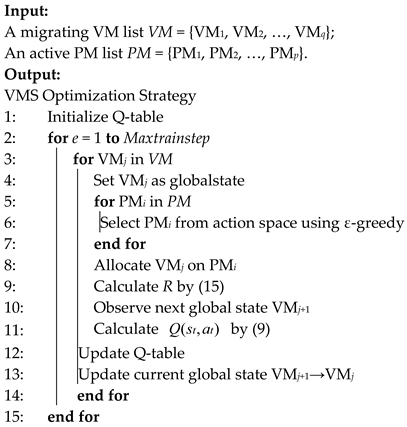
3.3. Proposed IVMS

In this subsection, the implementation of the Q-learning algorithm for VMS, which is the proposed IVMS, is shown as pseudocode below (Algorithm 1).

Algorithm 1: IVMS method

First, the Q-table is initialized to 0 or 1 depending on whether the PMs can meet the VM resource requirements. Then, each VM in the VM(t) is selected in turn (lines 1–4). For the current PM set PMs(t), the PM pm_s is selected by using the ε-greedy strategy (lines 5–7). After that, the next state will be observed to calculate its fitness value after assigning vm_q to PM pm_s to obtain the reward, and the Q-value of the current state is calculated by (15) (lines 8–11). Finally, after updating the Q-table value, the next VM will be selected at the next iteration and the algorithm flow will be executed again until the termination condition is satisfied (lines 12–15).

4. Experiment and Simulation

In this section, we describe the experiments we conducted on virtual machine optimization consolidation using a real private cloud platform experimental environment and a larger scale simulation by using the cloud computing simulation tool CloudSim 3.0.3.

4.1. Experiment Based on Cloud Platform

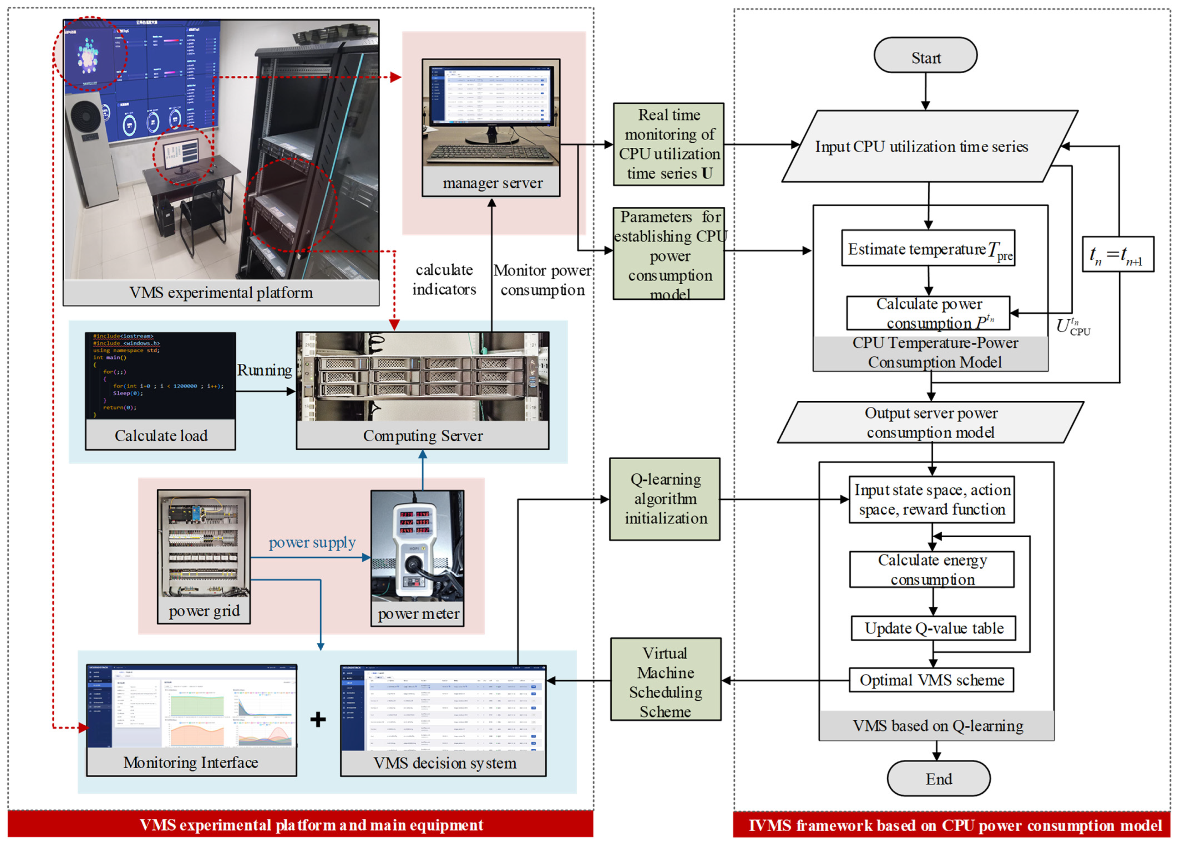
The experiment was conducted on the experiment cloud platform of the School of Electrical Automation and Information Engineering of Tianjin University. This cloud platform was built according to the cloud data center, which consists of six servers (NF5280F5, Inspur, Jinan, China) and one network switch (S6730-S24X6Q, Huawei, Beijing, China). There was a cloud management platform, which was used to manage PM clusters and loads. The process of designing the entire cloud platform and implementing virtual machine scheduling is shown in Figure 3. Based on this cloud platform PM cluster, this study conducted experiments of larger scales with the data from the PlanetLab dataset.

The experiment selected the running data of a cluster containing 60 PMs and 210 virtual machines in the PlanetLab dataset as the raw data for the experiment, which includes the CPU usage of each PM within 24 h. Subsequently, 60 sets of raw data were randomly averaged into six sets of CPU usage datasets, which were used as inputs for six PMs in the experimental platform. The experiment used load running tools to occupy the CPU usage of the PMs and simulate their actual resource usage when running cloud services. The experiment conducted four virtual machine scheduling sessions throughout the entire experimental cycle, with a scheduling policy execution cycle of 6 h. The virtual machine scheduling was performed at the 2nd, 8th, 14th, and 20th hours of the experiment.

At the same time, in order to characterize cloud business environments with different levels of busyness, we selected four sets of typical load situations as the input for the experiment. The difference between them lies in the difference in the average load level of the cluster, which can represent four typical working conditions of the data center cluster, namely lightly loaded, normally loaded, medium-loaded, and heavily loaded. The specific settings are shown in

Table 1. Average load levels of clusters selected for the experiment.

Cluster Average Load Level	Cluster Average Load Rate (CPU)
① lightly loaded	28%
② normally loaded	51%
③ medium-loaded	74%
④ heavily loaded	88%

.

Based on the above experimental setup, three different methods were used to generate virtual machine integration strategies. The first method is to combine the traditional linear server power load model with the classic BFD method (L-B), the second method is to combine the SPL model constructed in this paper with the BFD method (SPL-B), and the third method is the IVMS presented in this paper, which combines the SPL model with the Q-learning method (SPL-Q). Based on these three methods of computational optimization, different virtual machine layout strategies will be provided. Compared to the original situation without migration, the strategies obtained by the three methods have significant energy-saving effects. 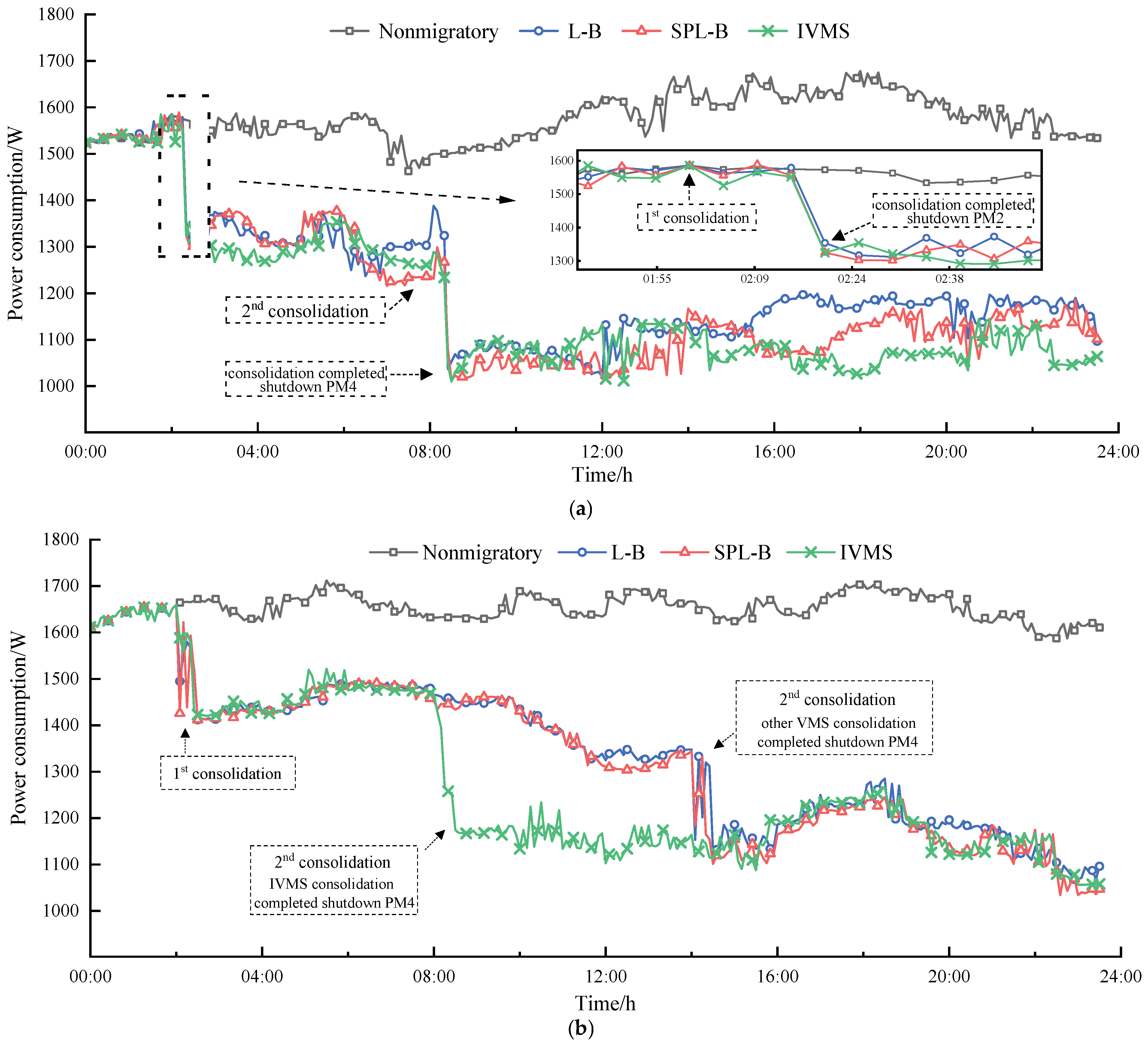Figure 4 shows the power consumption of a PM cluster optimized for a virtual machine layout using the three methods within 24 h at the four load rate levels mentioned above.

Figure 4, as well as Figure A1, show the changes in system power consumption after virtual machine integration using L-B, SPL-B, and IVMS under four different loads during a 24 h experimental period. Figure 4a shows that under the lightly loaded situation, at 2:00 and 8:00, our virtual machine scheduling framework monitors and determines that PM2 and PM4 are in a low-load state based on the current system resource usage, and the other four PMs have sufficient resources to accommodate all virtual machines on PM2 and PM4. Therefore, we have calculated a virtual machine migration plan, guided the virtual machine migration, and put the empty PM to sleep to achieve resource reallocation. It can be seen that at the above two moments, the virtual machine scheduling scheme is generated and executed. After a short period of time, PM2 and PM4 are shut down one by one. In the following time, the power consumption of the entire cluster system is significantly reduced. It is worth noting that the significant drop in power did not occur at the two sharp points of 2:00 and 8:00. This is because at sharp points, the scheduling program only completed the judgment of whether the system needs to perform virtual machine migration and integration based on system operation information. The judgment result is that optimization calculations and virtual machine migration after migration require a certain amount of time. In our laboratory, this process usually takes about 10 min.

From Figure 4b, it can be seen that under constant load conditions, the VMS framework proposed in this paper produces significantly different results compared to other VMS frameworks. Specifically, although the virtual machine migration integration schemes provided by the three VMS frameworks will perform some VM migration and shut down PM4 at the scheduled time of 2:00, at the scheduled time of 8:00, IVMS will further migrate the virtual machine and make PM2 idle and shut down. However, other VMS frameworks did not make such judgments and migration instructions but instead provided a certain VM migration scheduling scheme and operation at 14:00 in the next scheduling time, ultimately resulting in significantly higher overall system power consumption than the scheme provided by IVMS.

The experiment compared three different combinations of models and algorithms in terms of energy efficiency improvement. It can be seen that when the system is in a light-load state, using our scheduling framework to integrate computing resources has the most significant energy-saving effect, and as the load level increases, the energy-saving effect weakens. The reason is that when the load is low, the scheduling framework can integrate and concentrate more virtual machines, effectively reducing the use of real PMs. For example, in a light-load scenario with an average load rate of 38%, resource integration was achieved through scheduling virtual machines during the experiment. Two PMs are shut down sequentially without redundancy, greatly reducing system energy consumption. When the load is high, only effective virtual machine migration can achieve resource rearrangement, which may not reduce the actual number of running PMs. Therefore, the results of integrated optimization are only reflected in the resource layout, and it is difficult to significantly reduce energy consumption by reducing the number of PMs. For example, in an overload situation with an average load rate of 88%, even optimizing the resource layout through scheduling frameworks can only improve energy efficiency by about 2%.

In addition, as shown by the line in Figure 4, the virtual machine integration strategy that uses IVMS has significant energy-saving advantages compared to using only the more accurate SPL model or Q-learning algorithm, with an energy-saving effect of about 2.6–10.9%.

4.2. Simulation Based on CloudSim

To verify the effectiveness of the proposed framework and methodology in large-scale data center environments, most studies choose to conduct experiments on large-scale virtualized data center infrastructure simulation tools. A Java-based simulator developed by the CLOUDS Laboratory at the University of Melbourne called CloudSim provides an excellent platform. We conducted extensive experiments using CloudSim 3.0.3 to simulate real cloud data centers. It included a total of three physical machine models and four types of virtual machines. The specific configuration of PMs is shown in

Table 2. Configuration of PMs.

PMs	Cores	CPU	RAM	Operating System
A	8	Intel Xeon 3040 1.86 (GHz)	4GB DDR4 Dual Channel	Linux
B	8	Intel Xeon 3075 2.66 (GHz)	4GB DDR4 Dual Channel	Linux
C	16	Intel Xeon 3040 1.86 (GHz)	64GB DDR4 Dual Channel	Linux

. Similarly to Amazon EC2, we adopted several types of VMs according to [36].

Considering the complex environment in cloud computing, this experiment set up three types of workloads with different characteristics according to [37], assuming that the jobs are independent.

Figure 5 shows the comparison of system energy consumption after optimizing computing resources using L-B, SPL-B, and IVMS for large-scale simulation using CloudSim. It can be intuitively seen that the method proposed in this paper has the best effect in reducing energy consumption, significantly better than the other two methods. The green part in Figure 5 represents the system energy consumption optimized by IVMS, which is generally the lowest within 30 days. The red part indicates that SPL-B consumes more electricity than IVMS, the blue part indicates that L-B consumes more electricity than SPL-B, and the black part indicates the difference in energy consumption between using the traditional L-B method and not migrating.

Specifically, compared to not migrating virtual machines, the IVMS proposed in this paper saves about 17.8% of energy consumption, about 10.3% compared to the SPL-B method, and 7.5% compared to the traditional L-B method. The fundamental reason is that the server power consumption model considering temperature used in this paper is closer to the power consumption patterns in actual server workload fluctuations, which can provide assistance for more accurate decision-making in optimization. In addition, in the decision-making process of optimizing the layout of migrating virtual machines, the Q-learning method is used for global optimization, which greatly reduces the degree of resource fragmentation, makes the integrated PM cluster as close to the maximum limit as possible, ensures that computing resources are fully utilized, reduces redundancy, and thus improves the overall energy efficiency of the system.

5. Conclusions

In response to the energy-saving optimization problem of data centers, this paper improves the existing research that rarely uses accurate server power load models and constructs an SPL model. Based on this precise model, a virtual machine layout optimization problem model for cloud data centers was established. The new model can be solved using various algorithms. This paper uses the Q-learning method for solving this problem and proposes IVMS. The effectiveness of the new method is verified through experiments and simulations. At the same time, it is compared with traditional SPL models and traditional algorithms to prove the superiority of the new method in energy efficiency improvement. The generality of the method is verified through simulations of different scales.

The main research objective of this article is the virtual machine scheduling problem aimed at energy conservation. Through the scheduling of virtual machines and the integration of servers, the energy consumption of the entire system is minimized to the greatest extent possible. Energy conservation and consumption reduction are the focus and optimization goals of the system, so to some extent, the impact of system performance changes is ignored. The method proposed in this article has a good effect on the energy-saving operation of data centers, but there are certain limitations in optimizing data center operation. When considering the service quality and performance provided by the data center, the method proposed in this paper needs further optimization and adjustment, such as in the design of the penalty function in the Q-learning algorithm. In the future, we will adopt other more advanced solving algorithms or introduce resource utilization prediction as an input to the virtual machine scheduling framework, breaking through the limitations of the method proposed in this paper and achieving multi-objective optimization of energy efficiency and performance for computing clusters and data center systems.