
DDPG-ADRC-Based Load Frequency Control for Multi-Region Power Systems with Renewable Energy Sources and Energy Storage Equipment


Abstract
1. Introduction
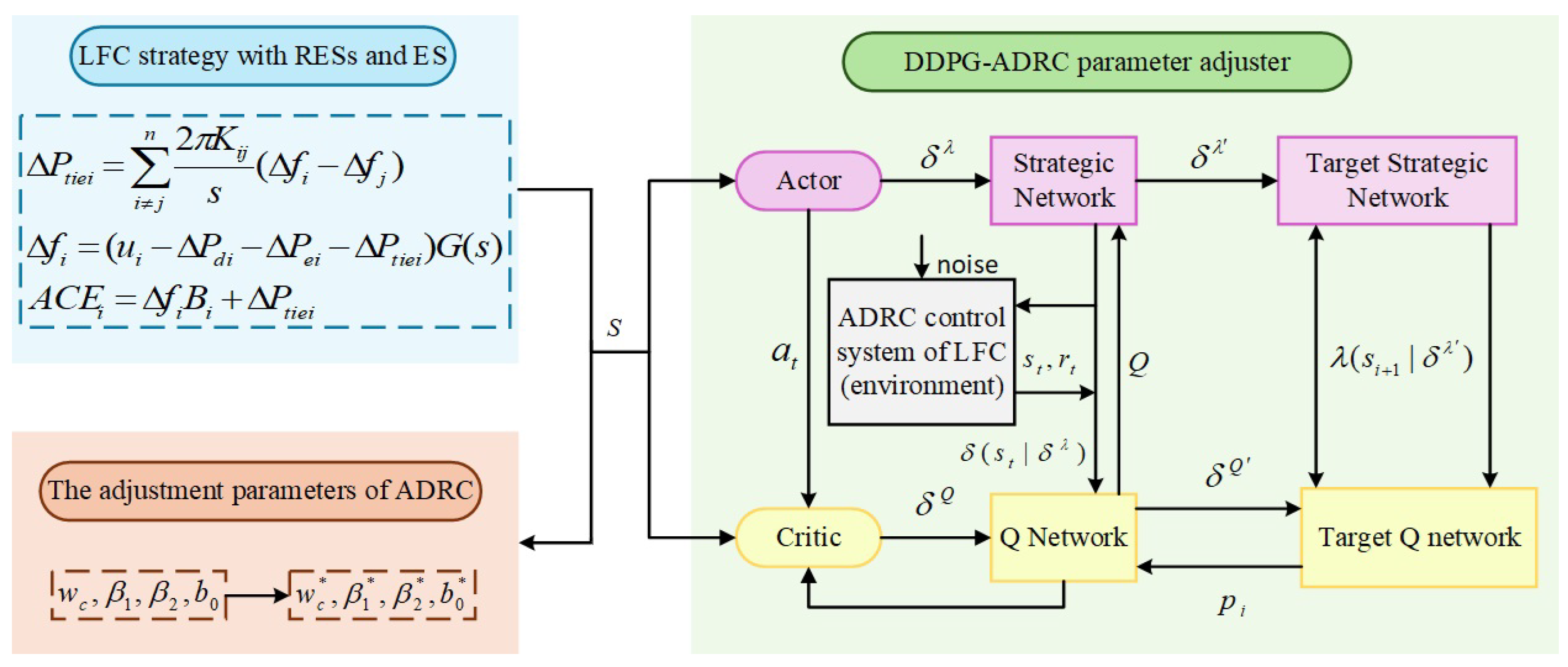
- This paper proposes an ADRC with a simple structure to enhance the system stability. Meanwhile, this article organically combines DDPG with ADRC, utilizing DDPG for the adaptive adjustment of key parameters in ADRC, thereby forming a novel LFC strategy.
- Compared with other methods [36,37,38,39], the method to optimize ADRC with DDPG proposed in this article has better anti-interference capability and is more suitable for dealing with uncertainties in multi-region power systems. In addition, relative to the solution without ES units, this method significantly enhances the transient response speed of the power system in the event of frequency deviation, which is improved by at least 15%.
2. System Model
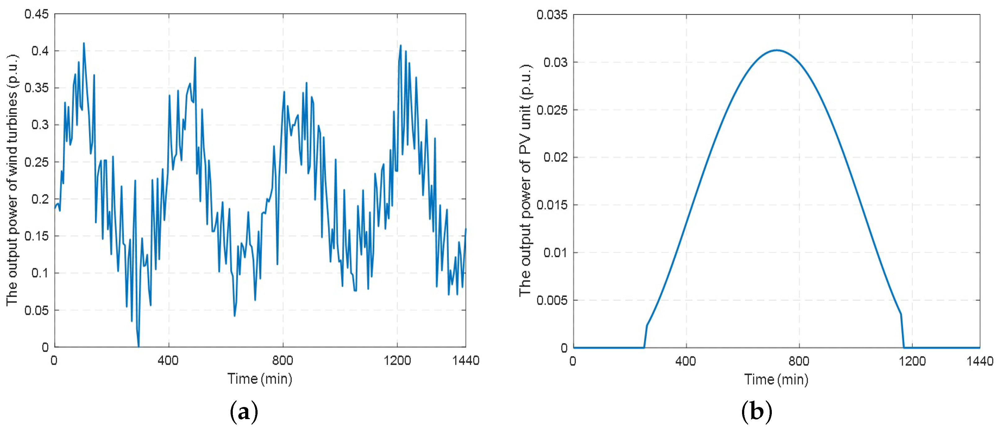
2.1. RESs Modeling
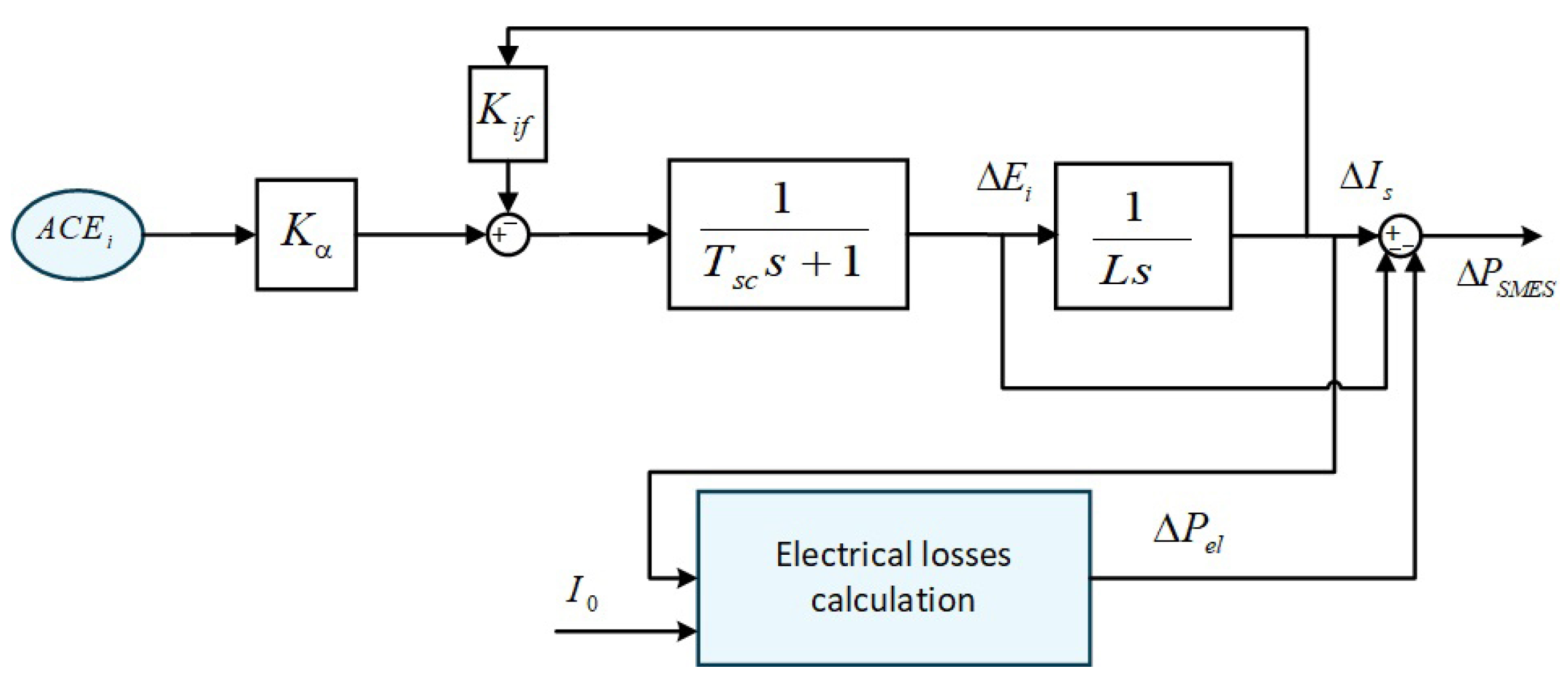
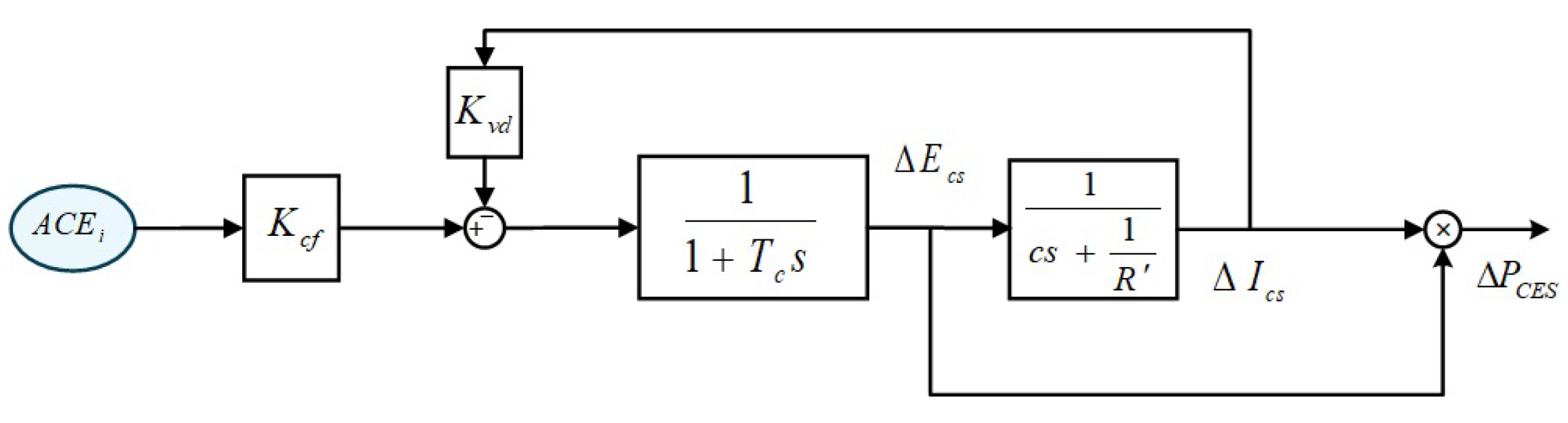
2.2. ES Equipment Modeling
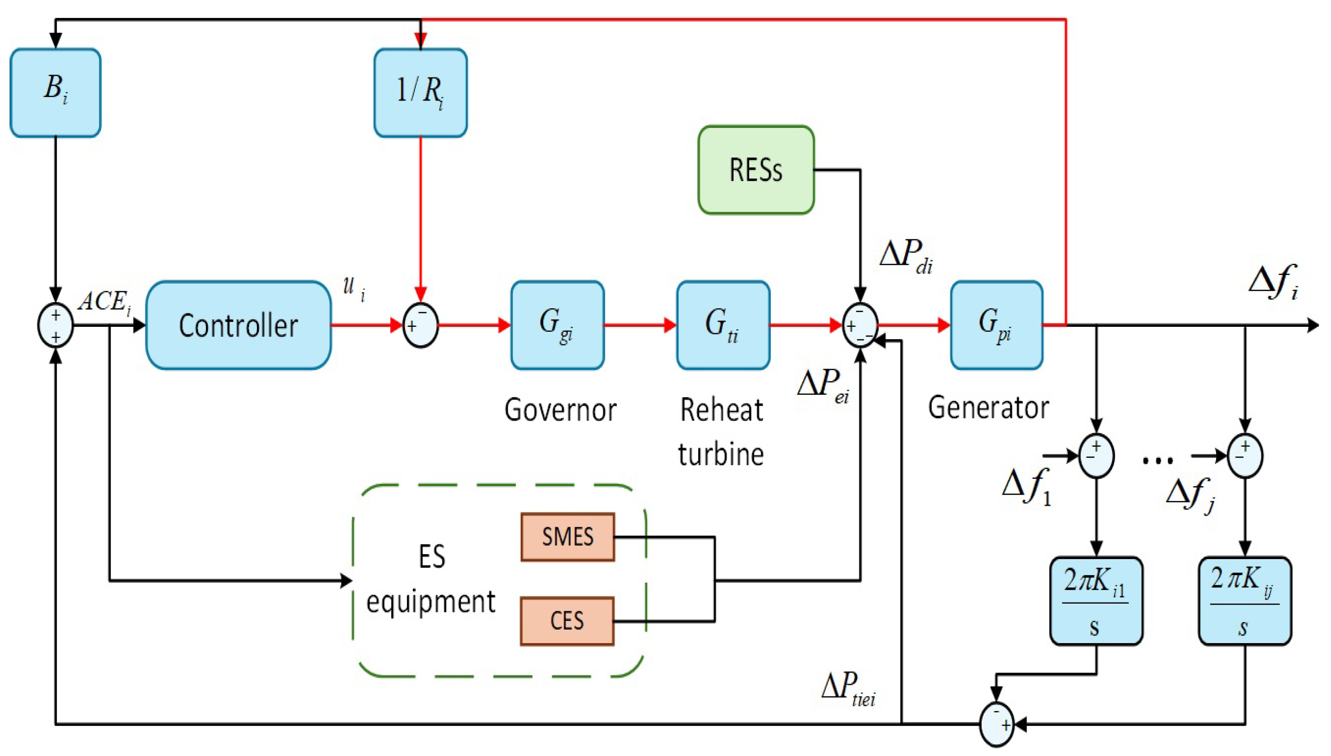
2.3. LFC Model of Power System
3. DDPG-ADRC Framework
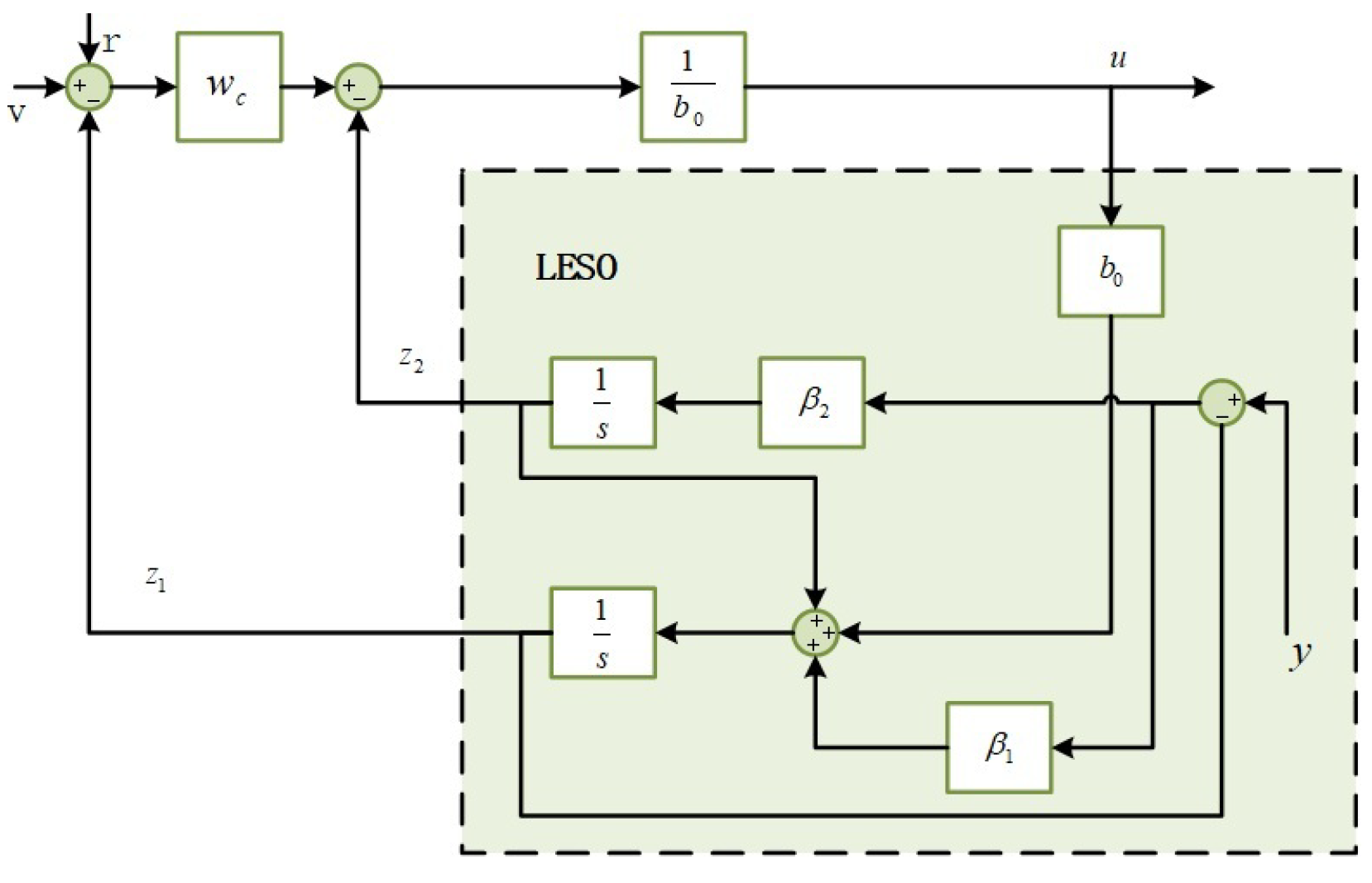
3.1. Design of First-Order ADRC
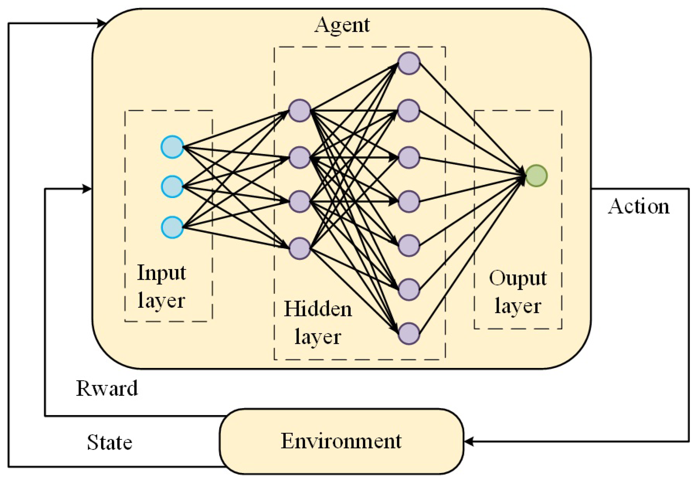
3.2. DDPG-Based Parameter Adjuster
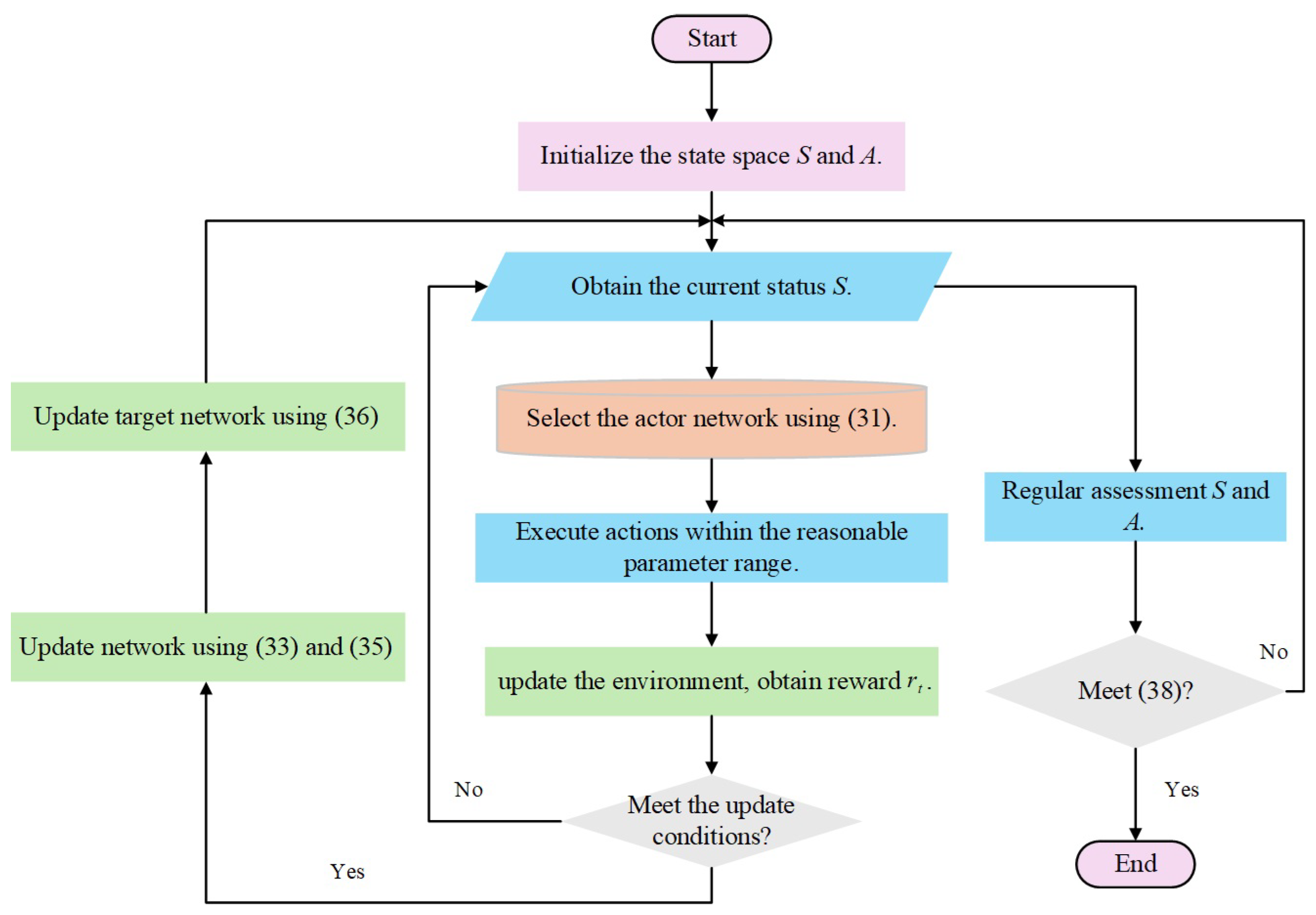
3.3. Parameter Optimization
4. Simulation Results
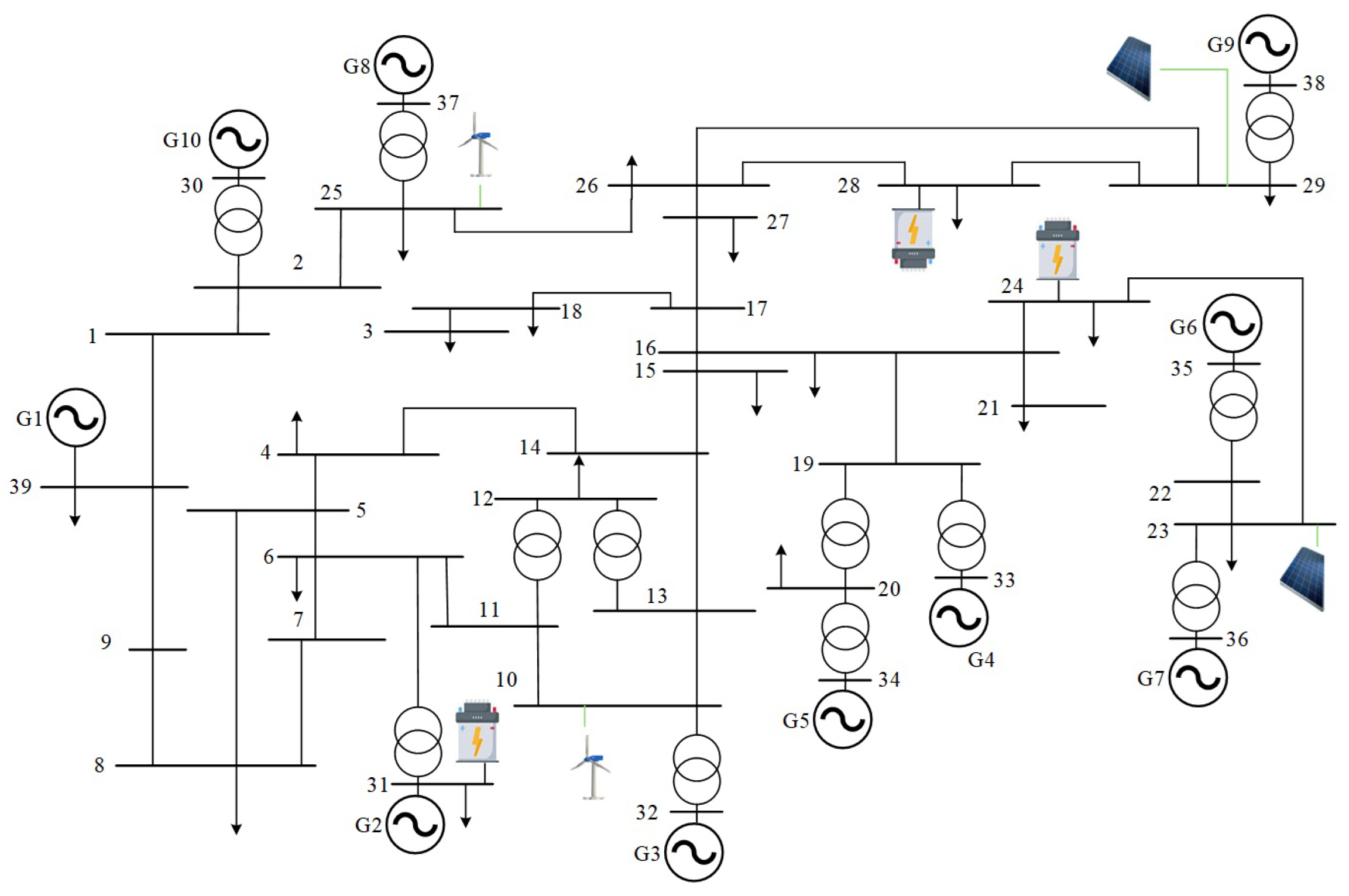
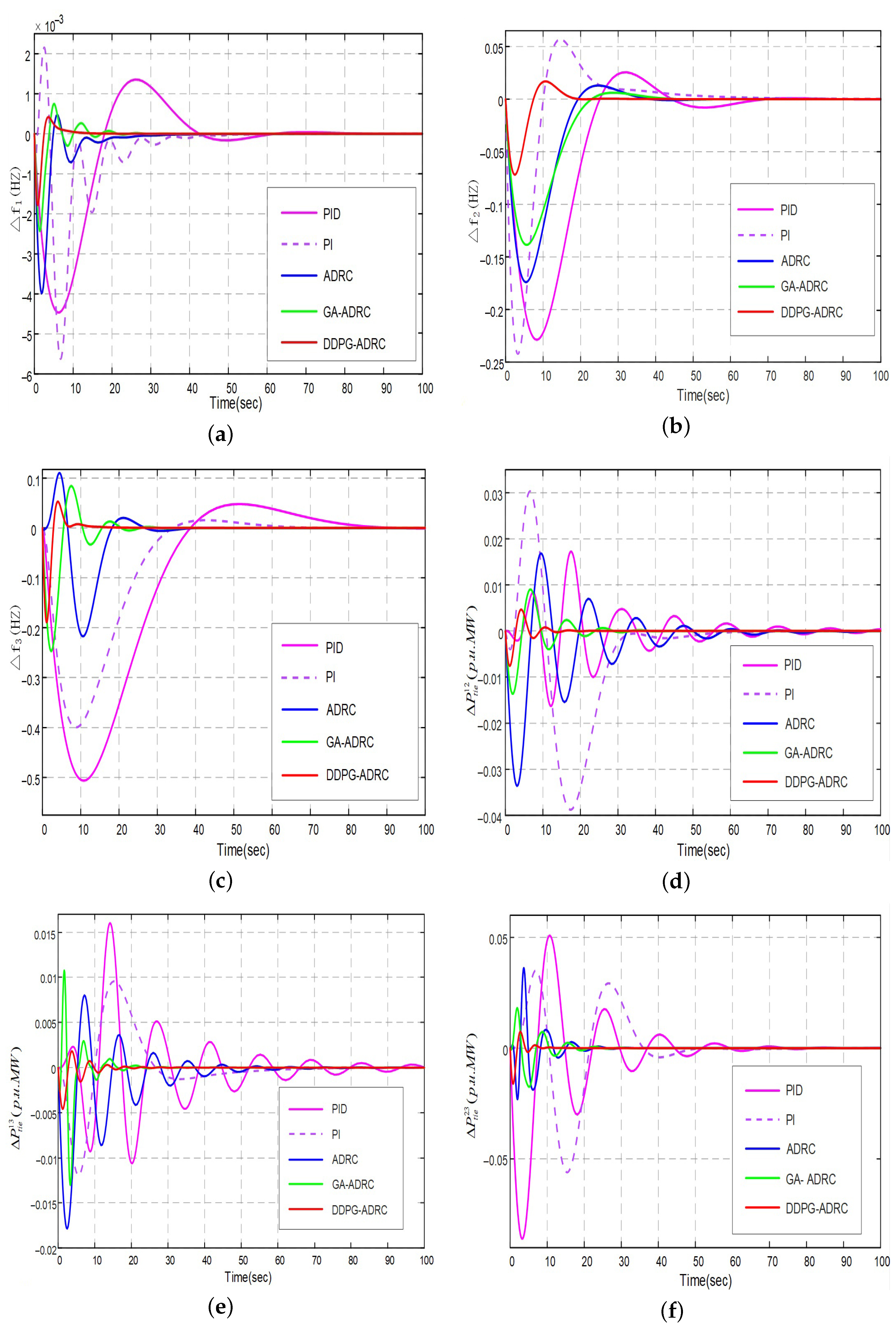
4.1. Three-Region Interconnected Power System Without ES
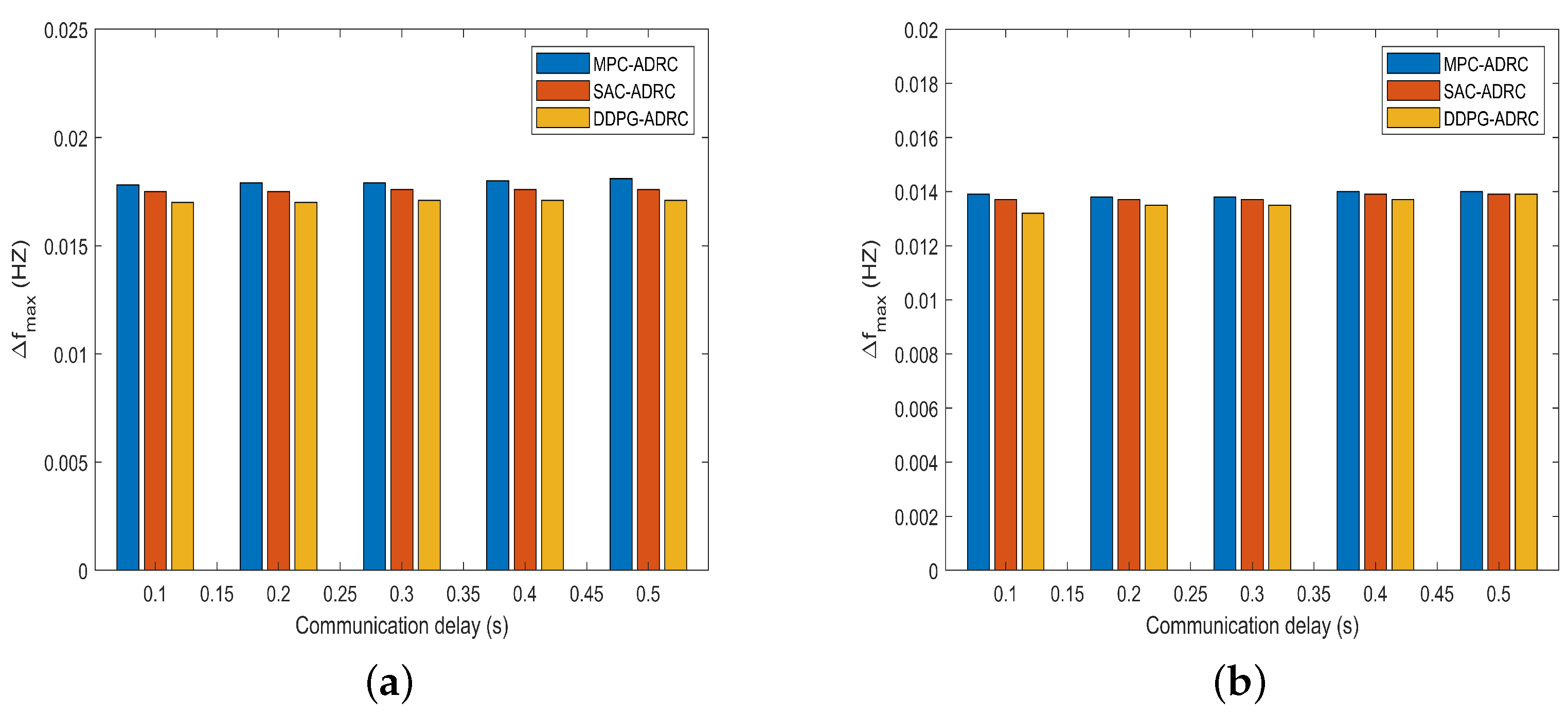
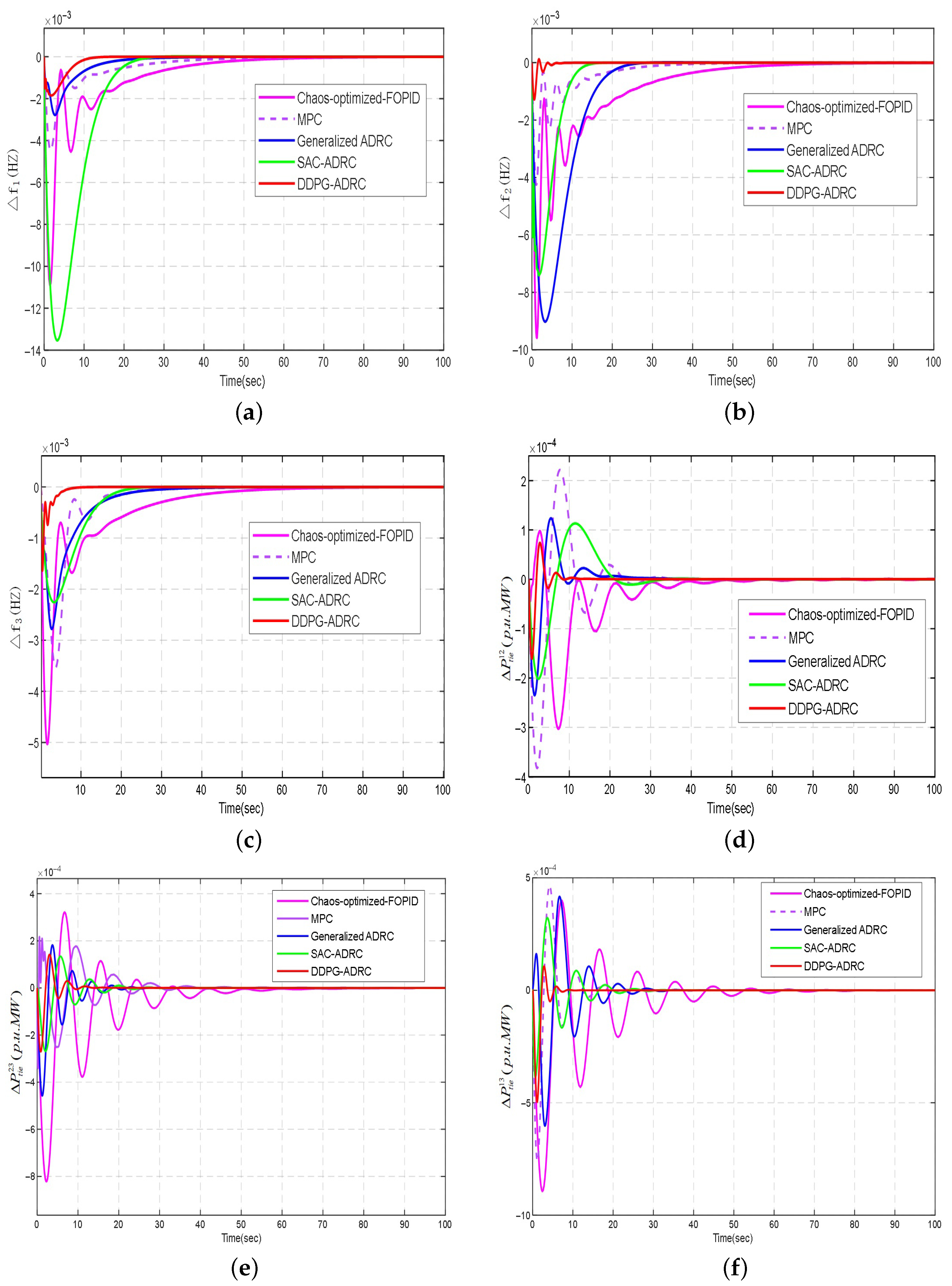
4.2. Performance Evaluation of the System Under Communication Delays
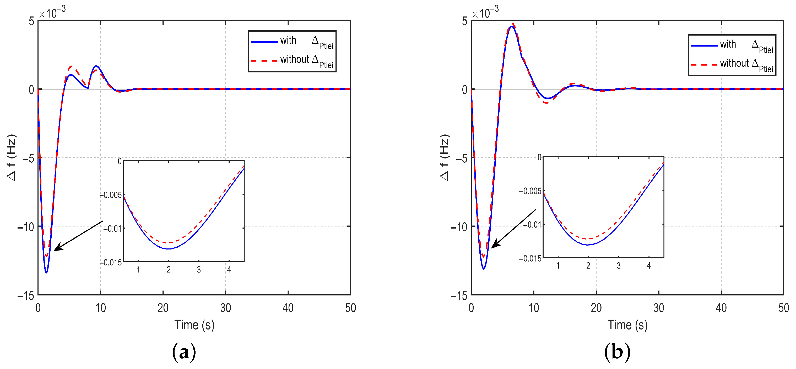
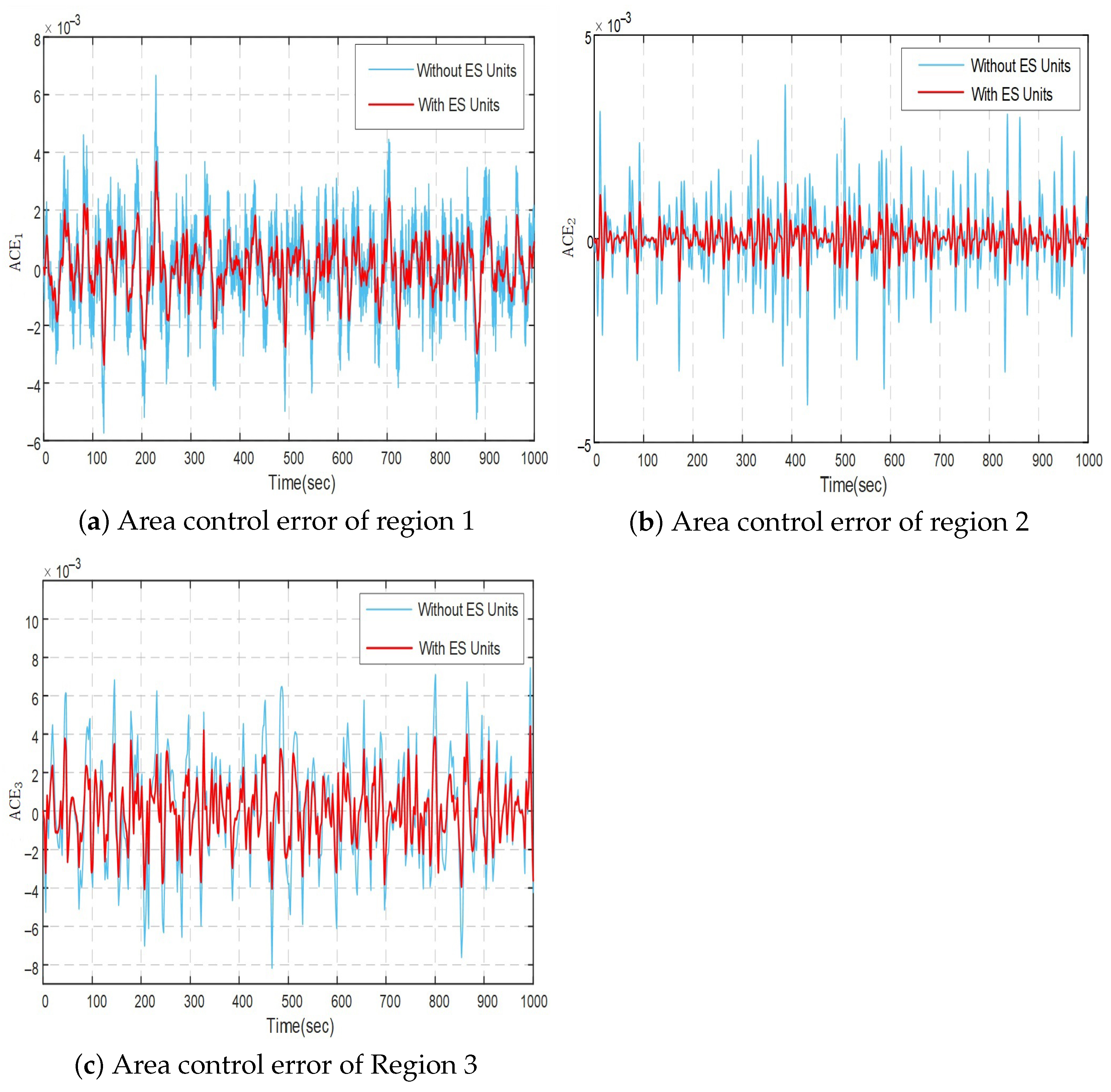
4.3. System Performance Evaluation with ES
5. Conclusions
Author Contributions
Funding
Data Availability Statement
Conflicts of Interest
References
- Liu, G.; Vrakopoulou, M.; Mancarella, P. Assessment of the capacity credit of renewables and storage in multi-area power systems. IEEE Trans. Power Syst. 2021, 36, 2334–2344. [Google Scholar]
- Mi, Y.; Ma, Y.; He, X.; Yang, X.; Gong, J.; Zhao, Y. Robust load frequency control for isolated microgrids based on double-loop compensation. CSEE J. Power Energy Syst. 2023, 9, 1359–1369. [Google Scholar]
- Li, M.; Zhang, Z.; Hu, S.; Lian, H. Sampling PI load frequency control for new energy power system. CSEE J. Power Energy Syst. 2023, 43, 939–950. [Google Scholar]
- Xia, K.S.; Liu, Y.; Wu, Q.H. Robust load frequency control of power systems against random time-delay attacks. IEEE Trans. Smart Grid 2021, 12, 909–911. [Google Scholar]
- Jia, Y.B.; Zhao, Y.D.; Sun, C.Y.; Meng, K. Cooperation-based distributed economic MPC for economic load dispatch and load frequency control of interconnected power systems. IEEE Trans. Power Syst. 2019, 34, 3964–3966. [Google Scholar]
- Babu, N.R.; Bhagat, S.K.; Chiranjeevi, T.; Pushkarna, M.; Saha, A.; Kotb, H.; AboRas, K.M.; Alsaif, F.; Alsulamy, S.; Ghadi, Y.Y.; et al. Frequency control of a realistic dish stirling solar thermal system and accurate HVDC models using a cascaded FOPI-IDDN-based crow search algorithm. Int. J. Energy Res. 2023, 1, 9976375. [Google Scholar]
- Chen, P.; Liu, S.; Zhang, D.; Yu, L. Adaptive event-triggered decentralized dynamic output feedback control for load frequency regulation of power systems with communication delays. IEEE Trans. Syst. Man Cybern. Syst. 2022, 52, 5949–5961. [Google Scholar]
- Pathak, P.K.; Yadav, A.K. Fuzzy assisted optimal tilt control approach for LFC of renewable dominated micro-grid: A step towards grid decarbonization. Sustain. Energy Technol. Assessments 2023, 60, 103551. [Google Scholar]
- Zhang, Z.; Liao, S.; Sun, Y.; Xu, J.; Ke, D.; Wang, B. A parallel-type load damping factor controller for frequency regulation in power systems with high penetration of renewable energy sources. J. Mod. Power Syst. Clean Energy 2024, 12, 1019–1030. [Google Scholar]
- Liu, S.; You, H.H.; Li, J.L.; Kai, S.J.; Yang, L.Y. Active disturbance rejection control based distributed secondary control for a low-voltage DC microgrid. Sustain. Energy Grids Netw. 2021, 27, 100515. [Google Scholar]
- Cui, Y.; Yin, Z.; Luo, P.; Yuan, D.; Liu, J. Linear active disturbance rejection control of IPMSM based on quasi-proportional resonance and disturbance differential compensation linear extended state observer. IEEE Trans. Ind. Electron. 2024, 71, 11910–11924. [Google Scholar]
- Lin, S.; Cao, Y.; Li, C.; Wang, Z.; Shi, T.; Xia, C. Two-degree-of-freedom active disturbance rejection current control for permanent magnet synchronous motors. IEEE Trans. Power Electron. 2023, 38, 3640–3652. [Google Scholar]
- Xu, L.; Zhuo, S.; Liu, J.; Jin, S.; Huang, Y.F.; Gao, F. Advancement of active disturbance rejection control and its applications in power electronics. IEEE Trans. Ind. Appl. 2024, 60, 1680–1694. [Google Scholar]
- Meng, Q.; Hou, Z. Active disturbance rejection based repetitive learning control with applications in power inverters. IEEE Trans. Control Syst. Technol. 2021, 29, 2038–2048. [Google Scholar]
- Wang, Q.C.; Xu, H.C.; Pan, L.; Sun, L. Active disturbance rejection control of boiler forced draft system: A data-driven practice. Sustainability 2020, 12, 4171. [Google Scholar]
- Dong, Z.; Li, B.W.; Li, J.Y.; Guo, Z.W.; Huang, X.; Zhang, Y.; Zhang, Z. Flexible control of nuclear cogeneration plants for balancing intermittent renewables. Energy 2021, 221, 119906. [Google Scholar]
- Li, X.H.; Wang, W.; Fang, F.; Liu, J.Z.; Chen, Z. Improving active power regulation for wind turbine by phase leading cascaded error-based active disturbance rejection control and multi-objective optimization. Renew. Energy 2025, 243, 122629. [Google Scholar]
- Safiullah, S.; Rahman, A.; Lone, S.A.; Hussain, S.M.S. Novel COVID-19 based optimization algorithm (C-19BOA) for performance improvement of power systems. Sustainability 2022, 14, 14287. [Google Scholar]
- Jain, S.; Hote, Y.V. Design of improved nonlinear active disturbance rejection controller for hybrid microgrid with communication delay. IEEE Trans. Sustain. Energy 2022, 13, 1101–1111. [Google Scholar]
- Hosseini, S.A.; Toulabi, M.; Dobakhshari, A.S.; Ashouri-Zadeh, A.; Ranjbar, A.M. Delay compensation of demand response and adaptive disturbance rejection applied to power system frequency control. IEEE Trans. Power Syst. 2020, 35, 2037–2046. [Google Scholar]
- Xi, L.; Zhang, L.; Xu, Y.; Wang, S.; Yang, C. Automatic generation control based on multiple-step greedy attribute and multiple-level allocation strategy. CSEE J. Power Energy Syst. 2022, 8, 281–292. [Google Scholar]
- Chen, Z.Q.; Huang, Z.Y.; Sun, M.W.; Sun, Q.L. Active disturbance rejection control of load frequency based on big probability variation’s genetic algorithm for parameter optimization. CAAI Trans. Intell. Syst. 2020, 15, 41–49. [Google Scholar]
- Wang, Y.C.; Fang, S.H.; Hu, J.X.; Huang, D.M. Multiscenarios parameter optimization method for active disturbance rejection control of PMSM based on deep reinforcement learning. IEEE Trans. Ind. Electron. 2023, 70, 10957–10968. [Google Scholar]
- Wang, Y.C.; Fang, S.H.; Hu, J.X. Active disturbance rejection control based on deep reinforcement learning of PMSM for more electric aircraft. IEEE Trans. Power Electron. 2023, 38, 406–416. [Google Scholar]
- Jain, H.; Mather, B.; Jain, A.K. Grid-supportive loads-a new approach to increasing renewable energy in power systems. IEEE Trans. Smart Grid 2022, 13, 2959–2972. [Google Scholar]
- Yu, Y.J.; Cai, Z.F.; Liu, Y.C. Double deep Q-learning coordinated control of hybrid energy storage system in island micro-grid. Int. J. Energy Res. 2020, 45, 3315–3326. [Google Scholar]
- Gu, C.J.; Wang, J.X.; Yang, Q.; Wang, X.L. Assessing operational benefits of large-scale energy storage in power system: Comprehensive framework, quantitative analysis, and decoupling method. Int. J. Energy Res. 2021, 45, 10191–10207. [Google Scholar]
- Tang, Y.M.; Bai, Y.; Huang, C.Z.; Du, B. Linear active disturbance rejection-based load frequency control concerning high penetration of wind energy. Energy Convers. Manag. 2015, 95, 259–271. [Google Scholar]
- Ebrahimi, H.; Abapour, M.; Mohammadi-Ivatloo, B.; Golshannavaz, S.; Yazdaninejadi, A. Decentralized approach for security enhancement of wind-integrated energy systems coordinated with energy storages. Int. J. Energy Res. 2021, 46, 5006–5027. [Google Scholar]
- Jiang, S.; Xu, Y.; Li, G.; Xin, Y.; Wang, L. Coordinated control strategy of receiving-end fault ride-through for DC grid connected large-scale wind power. IEEE Trans. Power Deliv. 2022, 37, 2673–2683. [Google Scholar]
- Liu, J.; Yao, W.; Wen, J.; Fang, J.; Jiang, L.; He, H. Impact of power grid strength and PLL parameters on stability of grid-connected DFIG wind farm. IEEE Trans. Sustain. Energy 2020, 11, 545–557. [Google Scholar]
- Wang, W.; Liu, L.; Liu, J.; Chen, Z. Energy management and optimization of vehicle-to-grid systems for wind power integration. CSEE J. Power Energy Syst. 2021, 7, 172–180. [Google Scholar]
- Rouhanian, A.; Aliamooei-Lakeh, H.; Aliamooei-Lakeh, S.; Toulabi, M. Improved load frequency control in power systems with high penetration of wind farms using robust fuzzy controller. Electr. Power Syst. Res. 2023, 224, 109511. [Google Scholar]
- Ye, F.; Hu, Z.J. Robust load frequency control of interconnected power systems with back propagation neural network-proportional-integral-derivative-controlled wind power integration. Sustainability 2024, 16, 8062. [Google Scholar]
- Wang, P.; Guo, J.; Cheng, F.; Gu, Y.; Yuan, F.; Zhang, F. A MPC-based load frequency control considering wind power intelligent forecasting. Renew. Energy 2025, 244, 122636. [Google Scholar]
- Barakat, M. Novel chaos game optimization tuned-fractional-order PID fractional-order PI controller for load-frequency control of interconnected power systems. Prot. Control Mod. Power Syst. 2022, 7, 1–20. [Google Scholar]
- Jain, S.; Hote, Y.V. Generalized active disturbance rejection controller for load frequency control in power systems. IEEE Control Syst. Lett. 2020, 4, 73–78. [Google Scholar]
- Li, Z.; Li, X.; Lin, Y.; Wei, Y.; Li, Z.; Li, Z. Active disturbance rejection control for static power converters in flexible AC traction power supply systems. IEEE Trans. Energy Convers. 2022, 37, 2851–2862. [Google Scholar]
- Song, D.; Chang, Q.; Zheng, S.; Yang, S.; Yang, J.; Joo, Y.H. Adaptive model predictive control for yaw system of variable-speed wind turbines. J. Mod. Power Syst. Clean Energy 2021, 9, 219–224. [Google Scholar]
- Baškarad, T.; Holjevac, N.; Kuzle, I. Photovoltaic system control for power system frequency support in case of cascading events. IEEE Trans. Sustain. Energy 2023, 14, 1324–1334. [Google Scholar]
- Mekhamer, A.S.; Hasanien, H.M.; Alharbi, M. Coati optimization algorithm-based optimal frequency control of power systems including storage devices and electric vehicles. J. Energy Storage 2024, 93, 112367. [Google Scholar]
- Gulzar, M.M.; Sibtain, D.; Khalid, M. Cascaded fractional model predictive controller for load frequency control in multiarea hybrid renewable energy system with uncertainties. Int. J. Energy Res. 2023, 2023, 5999997. [Google Scholar]
- Du, X.B.; Guo, C.Y.; Zhao, C.Y. Hydropower units are modeled by HVDC transmission system and multi-band oscillation mode analysis. Autom. Electr. Power Syst. 2022, 46, 75–83. [Google Scholar]
- Yi, X.Q.; Wang, D.; Liu, H.T. Dynamic simulation model of medium-voltage DC generator set considering the speed regulation characteristics of prime mover. Trans. China Electrotech. Soc. 2024, 39, 2974–2983. [Google Scholar]
- Sun, L.; Xue, W.; Li, D.; Zhu, H.; Su, Z.G. Quantitative tuning of active disturbance rejection controller for FOPTD model with application to power plant control. IEEE Trans. Ind. Electron. 2022, 69, 805–815. [Google Scholar]

| Symbol | ||||
|---|---|---|---|---|
| Value | 75.62 | 37.21 | 4 | 150 |
| Symbol | |||||||||||
|---|---|---|---|---|---|---|---|---|---|---|---|
| Value | 2.4 | 3 | 120 | 0.58 | 10 | 0.1 | 0.2 | 20 | 0.3 | 0.08 | 0.03 |
| Parameters | Learning Rate (Actor) | Learning Rate (Critic) | Noise | Batch Size | ||
|---|---|---|---|---|---|---|
| Value | 0.2 | 64 | 0.99 |
| Symbol | ||||||||
|---|---|---|---|---|---|---|---|---|
| Value | 1.225 | 5905 | 10 m/s | 50 m | 15 rad/min | 3.6 | 8 | 0.421 |
| Index | Region | Traditional Methods | DDPG-ADRC | Improvement | |||
|---|---|---|---|---|---|---|---|
| PID | PI | ADRC | GA-ADRC | (%) | |||
| Rise time (s) | 2.30 | 2.25 | 2.10 | 2.05 | 1.25 | 40.5 | |
| 2.45 | 2.40 | 2.25 | 2.20 | 1.35 | 40.0 | ||
| 2.20 | 2.15 | 2.05 | 1.95 | 1.20 | 41.5 | ||
| 0.95 | 0.90 | 0.85 | 0.80 | 0.45 | 47.1 | ||
| Settling time (s) | 9.20 | 8.80 | 8.50 | 8.30 | 4.20 | 45.8 | |
| 9.60 | 9.30 | 9.00 | 8.70 | 4.50 | 45.8 | ||
| 8.80 | 8.50 | 8.20 | 8.00 | 4.00 | 46.2 | ||
| 4.20 | 4.00 | 3.80 | 3.60 | 1.90 | 45.8 | ||
| Overshoot (%) | 21.5 | 20.0 | 18.5 | 16.0 | 4.2 | 60.0 | |
| 22.2 | 20.8 | 19.2 | 16.5 | 4.5 | 60.2 | ||
| 20.5 | 19.0 | 17.8 | 15.2 | 3.8 | 60.1 | ||
| 14.5 | 13.2 | 12.0 | 10.5 | 2.5 | 60.0 | ||
| ACE | 1 | 0.98 | 0.92 | 0.85 | 0.78 | 0.32 | 62.4 |
| 2 | 1.05 | 0.98 | 0.92 | 0.85 | 0.35 | 62.0 | |
| 3 | 0.92 | 0.85 | 0.78 | 0.70 | 0.28 | 64.1 | |
| Symbol | h | |||||
|---|---|---|---|---|---|---|
| Value | 0.4 kV/kA | 0.18 | 1.8 | 0.625 m | 2.412 m | 0.517 m |
| Symbol | L | |||||
| Value | 2 | 5000 A | 150 | 100 KV/p.u. MW | 3.4 H | 0.3 s |
| Symbol | c | |||||
| Value | 1.5 F | 80 | 0.05 s | 100 KA/p.u. MW | 0.25 KA/KV |
| Index | Region | Other Methods | DDPG-ADRC | Improvement | |||
|---|---|---|---|---|---|---|---|
|
Chaos- optimized- FOFID | MPC | Geralized ADRC | SAC- ADRC | (%) | |||
| Rise time (s) | 1.95 | 1.90 | 1.85 | 1.80 | 1.25 | 30.6 | |
| 2.10 | 2.05 | 2.00 | 1.95 | 1.35 | 30.8 | ||
| 1.85 | 1.80 | 1.75 | 1.70 | 1.20 | 29.4 | ||
| 0.70 | 0.65 | 0.60 | 0.55 | 0.45 | 18.2 | ||
| Settling time (s) | 7.80 | 7.50 | 7.20 | 7.00 | 4.20 | 40.0 | |
| 8.10 | 7.80 | 7.50 | 7.30 | 4.50 | 38.4 | ||
| 7.20 | 6.90 | 6.60 | 6.40 | 4.00 | 37.5 | ||
| 3.30 | 3.10 | 2.90 | 2.70 | 1.90 | 29.6 | ||
| Overshoot (%) | 14.5 | 13.8 | 13.0 | 12.2 | 4.2 | 65.6 | |
| 15.2 | 14.5 | 13.8 | 13.0 | 4.5 | 65.4 | ||
| 13.8 | 13.0 | 12.2 | 11.5 | 3.8 | 67.0 | ||
| 9.5 | 9.0 | 8.5 | 8.0 | 2.5 | 68.8 | ||
| ACE | 1 | 0.72 | 0.68 | 0.65 | 0.60 | 0.32 | 46.7 |
| 2 | 0.78 | 0.74 | 0.70 | 0.65 | 0.35 | 46.2 | |
| 3 | 0.65 | 0.62 | 0.58 | 0.54 | 0.28 | 48.1 | |
Disclaimer/Publisher’s Note: The statements, opinions and data contained in all publications are solely those of the individual author(s) and contributor(s) and not of MDPI and/or the editor(s). MDPI and/or the editor(s) disclaim responsibility for any injury to people or property resulting from any ideas, methods, instructions or products referred to in the content. |
© 2025 by the authors. Licensee MDPI, Basel, Switzerland. This article is an open access article distributed under the terms and conditions of the Creative Commons Attribution (CC BY) license (https://creativecommons.org/licenses/by/4.0/).
Share and Cite
Dou, Z.; Zhang, C.; Zhou, X.; Gao, D.; Liu, X. DDPG-ADRC-Based Load Frequency Control for Multi-Region Power Systems with Renewable Energy Sources and Energy Storage Equipment. Energies 2025, 18, 3610. https://doi.org/10.3390/en18143610
Dou Z, Zhang C, Zhou X, Gao D, Liu X. DDPG-ADRC-Based Load Frequency Control for Multi-Region Power Systems with Renewable Energy Sources and Energy Storage Equipment. Energies. 2025; 18(14):3610. https://doi.org/10.3390/en18143610
Chicago/Turabian StyleDou, Zhenlan, Chunyan Zhang, Xichao Zhou, Dan Gao, and Xinghua Liu. 2025. "DDPG-ADRC-Based Load Frequency Control for Multi-Region Power Systems with Renewable Energy Sources and Energy Storage Equipment" Energies 18, no. 14: 3610. https://doi.org/10.3390/en18143610
APA StyleDou, Z., Zhang, C., Zhou, X., Gao, D., & Liu, X. (2025). DDPG-ADRC-Based Load Frequency Control for Multi-Region Power Systems with Renewable Energy Sources and Energy Storage Equipment. Energies, 18(14), 3610. https://doi.org/10.3390/en18143610