Abstract
With the large-scale integration of converter-based renewable energy into power systems and the large-scale construction of HVDC, risks associated with supply–demand imbalance and post-contingency frequency instability of sending-end power grids have significantly escalated. This paper proposes a novel method for evaluating the regulation capacity requirements of sending-end grids, addressing both normal-state power balance and post-disturbance frequency security. In normal states, multiple flexible metrics that can quantify the supply–demand imbalance trend are introduced. Then, thermal power units and energy storage serve as the benchmark to quantify the specific capacity requirements. For post-contingencies, frequency security metrics are derived based on the system frequency dynamic model with synchronous generators, renewable energy, and energy storage. The derived frequency security metrics can quantify the credible frequency regulation capacity required to ensure system stability under a predefined disturbance. A multi-objective capacity requirement assessment model for both the normal state and the post-contingency frequency regulation is ultimately formulated to determine the minimum capacity requirements. The effectiveness of the proposed evaluation method is verified using the numerical simulation based on a practical sending-end grid.
1. Introduction
Governments pursue dual-carbon objectives and energy transition initiatives. Consequently, unprecedented amounts of renewable energy are now integrated into power grids. This integration exhibits accelerating growth rates []. In recent years, high-voltage direct current (HVDC) lines have been continuously constructed to transmit power from renewable-rich regions to load centers. The power grids in some regions of China have evolved into asynchronous multi-infeed HVDC systems with high penetration of renewable generation []. The escalating share of renewable energy has posed significant challenges in maintaining supply–demand. Consequently, flexibility requirements for accommodating net load variations are receiving widespread attention [].
Most of the existing studies address how much net load power demand can be handled by the existing resource portfolios. The study in [] analyzes and quantifies the available flexibility boundary of the system at a given operating point. An evaluation method for quantifying the available flexibility supply level of the system’s existing resources is proposed []. However, the above studies ignore multiple time periods and can only evaluate the supply–demand balance level at a given operating point. Therefore, some scholars have further studied the methods for quantifying the flexibility level of the system’s existing resources in multiple time periods, for instance, the system flexibility-level evaluation of existing units based on two-stage unit commitment []. Some other studies focus on enhancing the system’s supply–demand level by incorporating more flexible resources. The research in [,] evaluates the improvement effect of higher flexible resources based on the planning framework. However, the above-mentioned studies use the expected power curtailment framework to evaluate the available flexibility of the system’s existing resources or the available flexibility enhancement under a specific planning scheme. The exact flexibility capacity required to maintain supply–demand balance under specific net load conditions remains to be addressed. It is critically important for evaluating future grid operation schemes.
The replacement of synchronous generators (SGs) with converter-based RESs has significantly reduced system inertia levels and increased frequency instability risks under large disturbances []. Recent blackouts in South Australia and the UK were caused by insufficient system frequency support capabilities. These events demonstrate this critical phenomenon []. Current related studies focus on the optimization of unit commitment or dispatching schemes considering frequency security. The analytic model of traditional SGs’ frequency response was incorporated into the unit commitment [] and preliminarily verified the necessity for considering frequency security with predefined disturbances. As SGs are progressively displaced by renewable energy, expanding frequency support resources becomes imperative. The study of [] synthesizes control strategies enabling renewable units to provide frequency support, highlighting the promising application prospects of virtual synchronous generator control. The authors in [] integrate renewable units employing virtual synchronous generator control into conventional SG system frequency response models, demonstrating their significant operational cost benefits. However, to enable renewable participation in frequency support without curtailing wind power, the authors in [] integrate electrical energy storage frequency response models into frequency-security-constrained unit commitment. This demonstrates EES’s dual benefits: reducing operational costs and wind curtailment. Given the renewable generation’s growing dominance in modern power systems, incorporating its frequency support capabilities becomes essential for security. Thus, a multi-period operational optimization strategy coordinating SGs, renewables, and energy storage for frequency support is developed in []. Although the above work made significant contributions to coordinated operation for frequency security, the authors relied on the assumption of sufficient system frequency support capacity. The capacity requirements of multi-type resources participating in frequency regulation that the system needs to maintain frequency security during scenarios with inadequate frequency support capabilities is still an open challenge.
Therefore, this paper proposes a method for assessing the capacity requirements of the sending-end power grid from both the power balance of the normal state and the frequency security following credible contingency aspects. The proposed approach enables us to quantify how much capacity the system requires to handle the net load and maintain the system frequency security under disturbances for a certain multi-type resource combination scheme. A multi-objective assessment method for the minimum regulation capacity is proposed, considering the system supply–demand balance in the normal state, the operation characteristics of multi-type resources, and the frequency security-related constraints. The proposed method can intuitively quantify how much additional capacity of flexible resources the system needs to maintain the supply–demand balance of the system in the normal state, as well as the capacity demand for participating in frequency regulation to ensure the system’s frequency security. This method can provide a reference for the Transmission System Operator (TSO) to formulate planning schemes in the future.
The rest of this paper is organized as follows: multi-dimensional flexibility indices for the normal state and flexibility regulation capacity requirements model are established in Section 2. Section 3 derives the frequency security indices considering detailed frequency dynamics with frequency regulation of SGs, renewable energy, and energy storage. In Section 4, the assessment model of capacity requirements for both flexible regulation of normal power balance and frequency regulation under credible contingency is ultimately formulated, and the corresponding solution technique is also introduced. Case studies on a practical sending-end grid are analyzed in Section 5. Section 6 draws conclusions.
2. Quantitative Assessment Model for the Supply–Demand Balance in the Normal State
The existing generation mix scheme of the sending-end grid in this paper includes thermal units, wind turbines (WTs), and photovoltaic plants (PVs). The indices for the supply–demand balance in the normal state are first constructed to quantify the trend of supply–demand imbalance of the system under the existing unit mixing scheme in this section. Then, taking thermal units and electric energy storage as the benchmark of additional flexible regulation resources when there is a shortage in the system’s supply–demand balance, the requirements for the flexibility capacity in the normal state are quantified.
2.1. Supply–Demand Balance Indices in the Normal State
The multi-dimensional normal-state flexibility indices are constructed to quantify the capability to ensure system supply–demand balance under a given resource mix scheme, including upward/downward flexibility regulation, upward/downward flexibility expectation, and insufficient upward/downward flexibility duration ratio.
2.1.1. Upward/Downward Flexibility Regulation
When the system’s flexibility under the existing generation resource mix is insufficient, it will result in power curtailment. The upward/downward flexibility regulation and of the system at time t are determined based on the proportion of load shedding or renewable energy curtailment.
where denote the shedding amount of lth load and curtailment of wth WT and vth PV; represent the power demand of lth load and output of wth WT and vth PV.
2.1.2. Upward/Downward Flexibility Expectation
The expectation and of the system’s upward and downward flexibility can reflect the average level at which the power system maintains the supply–demand balance under the existing generation resource mix during the operation periods.
2.1.3. Upward/Downward Flexibility Duration Ratio
and represent the proportions of time with insufficient upward and downward flexibility, respectively, within operation periods. The calculation methods are as follows.
where and are the indicators of insufficient upward and downward flexibility at time t, respectively. if a load shedding event occurs at time t; if a curtailment event (WT or PV) occurs at time t.
2.2. Capacity Requirements for Flexibility Regulation
The capacity requirements for flexible regulation in a specific operating scenario refer to the additional regulation power required to ensure the supply–demand balance at time t when the available regulation capacity of the system is insufficient. The upward and downward regulation capacity requirements at time t are defined as and . The system’s upward regulation capacity requirement at time t based on power balance can be calculated as follows:
Similarly, the downward regulation capacity requirement at time t is
where represent the sets of SGs, WTs, PVs, tie lines, HVDC lines, and load, respectively; is the output of existing generation resources at time t; and are the powers transmitted outward through the tie lines and the HVDC lines, respectively, at time t.
Taking thermal units and electric energy storage as additional flexible regulation resources, and using their power output characteristics as the benchmark to quantify the capacity requirements for flexible regulation, the flexible regulation capacity requirements and of the system at time t are the aggregation of the power outputs of the additional flexible regulation resources.
Equation (10) indicates that the system’s downward regulation capacity requirements are the difference between the power output of the additional thermal units and the charging power of the eth energy storage, where is the discharging power of the eth energy storage. are the sets of additional thermal units and energy storage.
3. Frequency Regulation Reserve of Multi-Type Resources After Contingency
3.1. Frequency Response of Multi-Type Resources
PV plants can participate in frequency response by configuring a certain capacity of energy storage devices [], which provide inertial response and fast frequency regulation power support through the fast frequency response control strategy. Considering SGs, WTs, PVs, and electrical energy storage as the resources participating in frequency regulation, the system frequency dynamic model is as follows:
where is the power disturbance, is the system damping, represents the frequency deviation of the power grid at time t, represents the primary frequency regulation power provided by the ith resource at time t, and represents the equivalent inertia of the system.
The governors of SGs and WTs release the kinetic energy of the rotors by responding to real-time frequency deviations to suppress the rapid frequency drop. The primary frequency regulation response processes of SGs and WTs are approximated as linearly changing with time, and the expressions for the frequency regulation power provided by SGs and WTs are as follows []:
where are the frequency response power of gth SG and wth WT at time t, respectively; are the frequency regulation reserve of gth SG and wth WT at time t, respectively; represents the full-release time of the frequency regulation reserve.
Since energy storage devices can provide fast frequency regulation power support in milliseconds [], and their response time is much shorter than that of other resources, the response time of power release from energy storage and PV can be neglected. Therefore, their power responses can be superimposed on the active power disturbance side [], which can be expressed as follows:
where is the maximum discharge power of the eth energy storage device, and represents the frequency regulation response power of the energy storage at time t.
3.2. Frequency Regulation Reserve of Multi-Type Resources
When an active power disturbance occurs, the frequency regulation capability of SGs is related to the frequency deviation, their parameters, and the power output at time t. According to the Regulations of Grid-Connection Guidelines for Wind Farms in China [], when the generation power of a wind turbine reaches more than 20% of its capacity, a certain amount of capacity can be reserved for primary frequency regulation. In contrast, energy storage devices immediately release all their remaining available power. Based on this, the constraints on the primary frequency regulation reserve that SGs, WTs, and energy storage (PVs) can provide at time t are as follows:
where represents the droop coefficient of the SGs; denote the allowable maximum frequency deviation and the primary frequency regulation dead-band after a disturbance, respectively; is the curtailment coefficient of wth WT; is the installed capacity of wth WT; is the frequency regulation reserve of eth energy storage.
3.3. Frequency Security Indices
3.3.1. System Equivalent Inertia Level
According to the description of the frequency response control strategy for multi-type resources in Section 3.1, the equivalent inertia after aggregating the resources providing inertial response in Equation (11) can be calculated as follows:
where and are the inertial time constant and the installed capacity of the multi-type resources, respectively; is the commitment state of thermal units at time t.
3.3.2. Frequency Security Indices
In order to ensure the frequency security of the system after a disturbance, frequency security constraints need to be incorporated into the process of capacity requirement assessment. The system frequency security is ensured by imposing constraints on two key steady-state analytical indices that characterize the system frequency response process, namely, the maximum rate of frequency change and the maximum frequency deviation . The schematic diagram of the relationship between the above-mentioned indices and the system frequency dynamics in Equation (11) is shown in Figure 1.
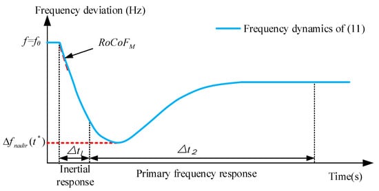
Figure 1.
The illustration for the relationship between frequency security indices and system frequency dynamics of (11).
The moment when the rate of frequency change reaches its maximum value is the initial transient moment after the disturbance occurs. At this time, the system frequency deviation is still 0. By substituting this condition into Equation (11), the analytical model of the maximum rate of frequency change can be derived.
where is the security threshold of the maximum rate of frequency change.
In order to feasibly obtain the linearized transient frequency deviation constraint, it is conservatively assumed that the frequency deviation is constrained without considering the system damping []. When the units provide primary frequency regulation, the time when the system reaches the maximum frequency deviation is less than the time when the frequency regulation reserve of the units is fully released. Otherwise, the system frequency will continue to decline. Therefore, the maximum frequency deviation and the corresponding time can be further derived after ignoring .
Substituting Equations (12) and (13) into Equation (11) and integrating both sides of Equation (11), we can obtain
The maximum frequency deviation occurs exactly at the moment when the rate of frequency change is 0. By setting , the time when the system frequency reaches nadir can be calculated.
4. Assessment of the Minimum System Regulation Capacity Requirements
Based on the proposed derivation and quantification method, system capacity requirements of normal state power balance and post-disturbance frequency regulation for frequency security can be further quantified by the quantification models in Section 2 and Section 3, respectively. The system frequency security is characterized by the frequency security indicators in Section 3. Among them, the equivalent inertia exactly includes the capacities of all resources that need to participate in the system frequency regulation. The regulation capacity model of normal-power balance and frequency regulation are combined in this section, and the overall assessment method that can determine the minimum capacity of both regulation states is formulated here.
4.1. Assessment Model
The system regulation capacity requirements include the flexible regulation capacity requirements for supply–demand balance in the normal state and the capacity requirements of multiple types of resources participating in frequency regulation for post-contingency frequency security. The flexible regulation capacity requirements in the normal state are uniformly defined as . Taking the equivalent inertia and the flexible regulation capacity as the assessment objectives, the minimum capacity requirement of the system is determined as follows:
The constraints include two categories: those of the normal operation state and those related to the post-contingency frequency security. The constraints for the normal operation state include the system power balance constraint (26).
When , represents the upward regulation capacity requirement . Conversely, when , represents . Then, Equations (9) and (10) can be uniformly expressed in terms of as follows:
Equations (28) and (29) restrict the power output range and ramping of the existing and additional thermal units, where and are the power output ranges of the thermal power units, respectively, and and are their ramp limits, respectively. Equations (30) and (31) limit the charging/discharging powers and states of the energy storage, where F is the charging and discharging state of the eth energy storage device at time t. In addition, the constraints in the normal state also include the unit commitment constraints of the thermal power units and the state of charge (SOC) constraints of the energy storage devices, which are the same as those in [].
By combining Equations (19)–(21) and substituting Equations (23) and (24) into Equation (22), the constraints of frequency security indices are transformed into the forms of system inertia requirement constraints (32) and (33), respectively:
Moreover, the frequency security-related constraints also include the frequency regulation reserve constraints (15)–(17) of multiple types of resources in Section 3.
4.2. Solution Technique
Since the objective function contains two sub-objectives, the overall evaluation model is a multi-objective optimization model. The NSGA-II algorithm is adopted to simultaneously optimize the two objective functions in the model. Based on the basic genetic algorithm (GA), three improvement measures, namely the fast non-dominated sorting algorithm, the elitist strategy, and the crowding degree comparison operator, are employed. These measures can accelerate computational efficiency and improve convergence robustness but do not alter Pareto-optimal outcomes. The algorithm flow chart is shown in Figure 2.
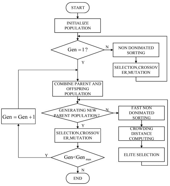
Figure 2.
Flow chart of the NSGA-II algorithm.
After generating the Pareto front through multiple iterations, an evaluation function is defined based on the weight coefficients of different objectives:
where represents the Pareto solution set; and are the weight coefficients of the two objective functions; and are the function values of different optimization objectives under the current solution; and are the maximum values of the corresponding objectives in the Pareto solution set.
5. Case Study
5.1. Case Settings
The sending-end power grid in China is used as a test system to verify the effectiveness of the proposed method. The grid topology is presented in Figure 3. The topology of the test system is equivalent to containing 10 key nodes with 500 kV voltage levels and 11 AC transmission lines. And its combination of power generation resource types, including SGs, WT, and PV. The system conducts power exchange with Region A and Region B via three HVDC lines and is connected to Region C through an AC tie-line with a capacity of 500 MW. We tested the capacity requirements of the multi-type resource mix schemes for the system in two stages.
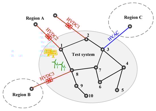
Figure 3.
The grid topology of the test system.
The load and generation resource mix schemes for the two stages are shown in Figure 4. The system of stage 1 includes 6 SGs (3 coal-fired and 3 gas-fired), 6 WTs, and 7 PVs, and their detailed grid-connection nodes and installed capacity are shown in Table 1. The capacity penetration levels of WT and PV are 21.22% and 24.76%, with a total of 45.97% of renewable units. In Phase 2, a 350 MW SG, a 200 MW WT, and two 200 MW PV units are newly installed at Nodes 3, 2, 5, and 9, respectively. WTs at Nodes 7, 4, 6, and 10 will be simultaneously expanded to 325 MW, 275 MW, 200 MW, and 250 MW, respectively. And all PVs except the one at Node 5 of stage 1 will be, respectively, expanded to 500 MW, 500 MW, 300 MW, 300 MW, 300 MW, and 200 MW. The penetration of renewable energy will exceed 50%, with WTs and PVs increasing to 23.36% and 32.45%, respectively. The hourly ramp-up/-down of coal-fired and gas-fired generation is set to 0.3 and 0.5 of the capacity. The frequency regulation parameters and parameters of energy storage are the same as in [].
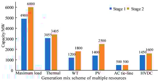
Figure 4.
The load and generation resource mix schemes of the two stages.

Table 1.
Detailed generation units of stage 1.
Two typical scenarios for load demand and power prediction of the two stages are selected as the input scenarios. It is expected that the proportion of externally transmitted power of the system will reach 25.6% and 38.65% in two stages. In Stage 1, the capacities of the three HVDC lines are 600 MW, 400 MW, and 450 MW, respectively. In Stage 2, the capacity of HVDC3 is expanded to 600 MW. The predefined disturbance is set as the bipole block of HVDC1.
5.2. Regulation Capacity Requirements of Scenario 1
Scenario 1 represents a typical operating scenario with a high annual load level. The system load demand and output prediction of renewable energy with a 95% confidence level are shown in Figure 5a. In Scenario 1, the daily power demand of the test system remains at a relatively high level throughout the day, and the load exhibits a double-peak characteristic. WTs have a relatively high generation level during the low-load periods, showing an anti-peak-shaving characteristic. During the noon peak periods (13:00–17:00), the power generation of PVs is relatively abundant, but the power generation of WTs is relatively small. During the evening peak periods (20:00–22:00), the output of both PV and WT is relatively small. Figure 5b shows the external power transmission requirements of the AC tie-lines and HVDC lines in Scenario 1. During the noon peak periods (13:00–17:00), all three DC lines are operating at full capacity. However, during the evening peak periods (20:00–22:00), the transmission capacity of HVDC 1 is relatively low. Therefore, it is more likely to encounter a shortage of upward flexibility regulation capacity in this scenario.
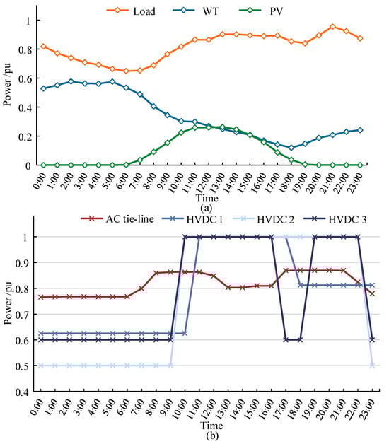
Figure 5.
The renewable energy output, power demand of load and external lines in Scenario 1. (a) power of renewable energy and load demand; (b) power demand of external lines.
The flexibility capacity requirements in the normal state and frequency regulation capacity requirements of the system for the two stages are shown in Figure 6. There are mainly upward flexibility gaps during the evening peak period in both stages. Compared with Stage 1, the maximum load in Stage 2 has increased by 1096 MW, but the newly added thermal power units of the existing generation mix scheme are only 350 MW. The power output of PVs is close to 0 during the evening peak periods (20:00–22:00), and the power output level of WTs is also at its lowest level throughout the day. Therefore, the upward flexibility shortage in Stage 2 has significantly increased, and it is difficult to meet the load demand relying solely on the existing generation mix scheme.
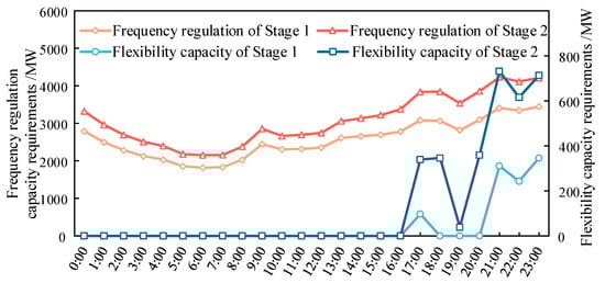
Figure 6.
Capacity requirements of two stages in Scenario 1.
The total capacity of multiple resources participating in frequency regulation of the system changes with the variation in the system load demand level. During the periods when the load demand is the smallest throughout the day (0:00–7:00), the total frequency regulation capacity of the system decreases as the load demand decreases. This is because the decrease in load allows each resource to reserve more frequency regulation reserve capacity to participate in frequency support, reducing the demand for the number of resources required to participate in frequency support, and thus reducing the total frequency regulation capacity requirements.
After 7:00, as the load demand increases, more power output from resources is used to ensure the supply–demand balance in the normal state, which in turn reduces the available frequency regulation response power of resources. More flexible resources are forced to participate in frequency support, so the total frequency regulation capacity increases. Similarly, during the evening peak period (20:00–22:00) when the load power demand is the highest, the frequency regulation capacity requirements of the system reach the highest level.
The flexibility level of the system without considering additional flexible resources is quantified based on the multi-dimensional flexibility indices in this paper. Figure 7 shows the flexibility regulation of the system. In Scenario 1, there is no insufficient downward flexibility in the system. There is insufficient upward flexibility during multiple periods in the scenarios. The upward flexibility level in Stage 1 is above 0.9, while in Stage 2, there are multiple periods when it is lower than 0.9. The computation results of the flexibility expectation and the flexibility duration ratio are shown in Table 2. The proportions of the time with insufficient upward flexibility of the system in Stage 1 and Stage 2 are 16.7% and 29.2%, respectively, and the expected level of upward flexibility within the periods in Stage 2 is also lower than that in Stage 1.
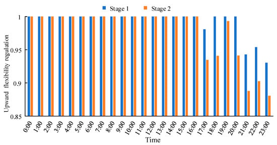
Figure 7.
System flexibility regulation of Scenario 1.
Table 2.
Supply–demand balance indices of Scenario 1.
5.3. Regulation Capacity Requirements of Scenario 2
Scenario 2 represents a typical scenario with a relatively low annual load level. The load demand, the output of renewable energy, and the externally transmitted power are shown in Figure 8. In Stage 1, the peak load is 2834.76 MW, and the valley load is 1615.31 MW. The early morning and afternoon periods are the low-load demand periods. There is a large power generation from WTs from 1:00 to 6:00, and a relatively high-power output from PVs from 11:00 to 17:00. The maximum penetration rates of asynchronous generation resources in the system for Stage 1 and Stage 2 are 73.48% and 68.50%, respectively, which occur at 15:00 and 14:00. At these times, there is insufficient space for renewable energy consumption. If no measures are taken, the curtailment of renewable energy will be 2102.2 MWh and 2637.2 MWh in Stage 1 and Stage 2, respectively.
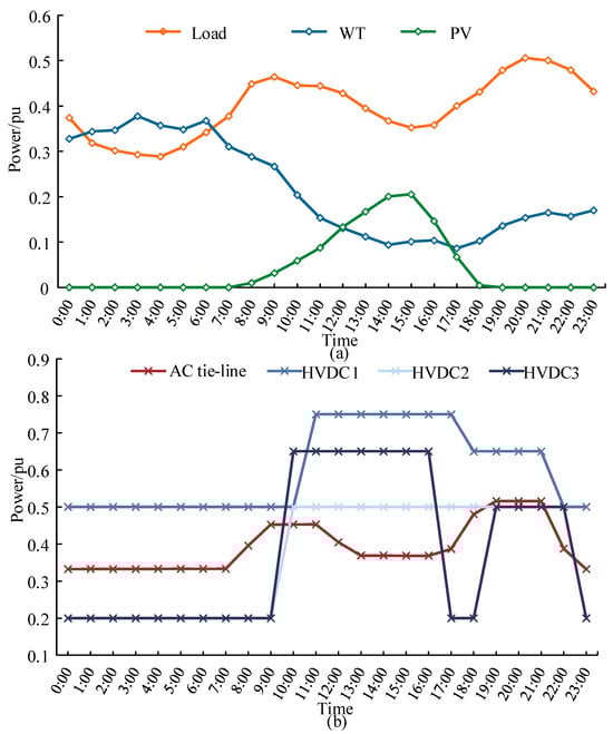
Figure 8.
The renewable energy output, power demand of load and external lines in Scenario 2. (a) power of renewable energy and load demand; (b) power demand of external lines.
The regulation capacity requirements in typical Scenario 2 are shown in Figure 9. There is no shortage of upward flexibility regulation capacity in both stages in Scenario 2. However, there is a significant shortage of downward flexibility regulation capacity during the periods of 1:00–5:00 and 13:00–16:00. The maximum requirements for downward regulation capacity in the early morning period occur at 3:00, which is mainly caused by the relatively low load demand level and the large power generation from WTs. Compared with Stage 1, the installed capacities of WTs and PVs in the test system of Stage 2 increase by 600 MW and 1100 MW, respectively. The peak load in Stage 2 increases by 607.45 MW compared with that in Stage 1, and the valley load increases by 346.1 MW compared with that in Stage 1. Therefore, the demand capacities for downward regulation from 1:00 to 5:00 and from 13:00 to 16:00 in Stage 2 are slightly higher than those in Stage 1.
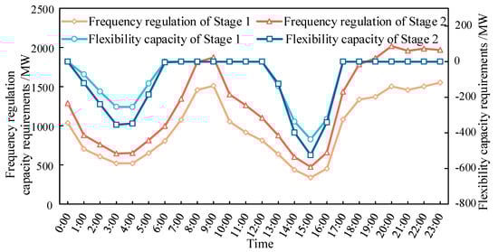
Figure 9.
Capacity requirements of two stages in Scenario 2.
The flexibility regulation of the system is shown in Figure 10. There is no upward insufficient upward flexibility in the system. If additional flexible resources are not considered, the downward flexibility of the system is at a relatively low level during the early morning and afternoon periods. Even the curtailment rate of renewable energy within the region is relatively high during the low-load periods of 14:00–16:00 in Stage 1. In Stage 2, due to the increase in the system load demand, the downward flexibility levels at multiple periods are slightly improved compared with those in Stage 1. The computation results of the flexibility expectation and the flexibility duration ratio are shown in Table 3. The downward flexibility duration ratio of the system in Stage 1 and Stage 2 is 37.5% and 41.7%, respectively. The downward flexibility expectation in Stage 2 increases by 4.8% compared with that in Stage 1, and the curtailment rate of renewable energy decreases by 6.24%.
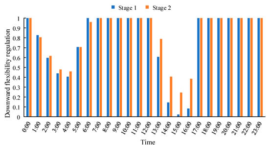
Figure 10.
System flexibility regulation of Scenario 2.
Table 3.
Supply–demand balance indices of Scenario 2.
5.4. Frequency Security Performance
The minimum inertia demand level of the system, computed based on the two frequency security index limits in typical Scenario 1 and the equivalent inertia of the system obtained from the assessment model, is shown in Figure 11. During the periods from 11:00 to 17:00, the transmission power of HVDC1 is relatively high. If a bipolar blocking event occurs at these times, the active power deficit in the system will be larger. The minimum inertia demand of the system is relatively high during these periods. The thermal power units with large online capacities provide a relatively sufficient rotational inertia. Therefore, after quantifying the frequency regulation capacity demand of the system, the equivalent inertia obtained from the assessment model can meet the minimum inertia level required for the system frequency security. Thus, it can be seen that the system inertia level will be maintained at a relatively high level as much as possible to ensure the system frequency security after considering the constraints of the two frequency security indices in the form of inertia.
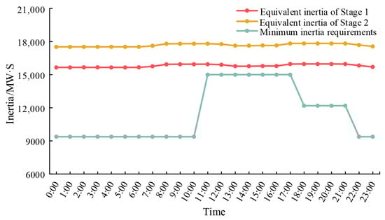
Figure 11.
The system inertia level of Scenario 1.
5.5. Solution Performance of the Algorithm
The Pareto solution set of the system capacity requirements at 15:00 solved by the NSGA-II algorithm in Scenario 2 is shown in Figure 12a. The weight coefficients of both objectives are set to 0.5. The optimal point can be selected from the Pareto solution set through the evaluation function defined in the previous text (the minimum inertia representing frequency security capacity requirement is 11,835.145, and the minimum flexibility regulation capacity requirement is 207.104 MW). Similarly, the corresponding Pareto solution set at 20:00 is shown in Figure 12b. The minimum inertia requirement at this time is 11,336.261, and the flexibility capacity requirement is 400.581 MW.
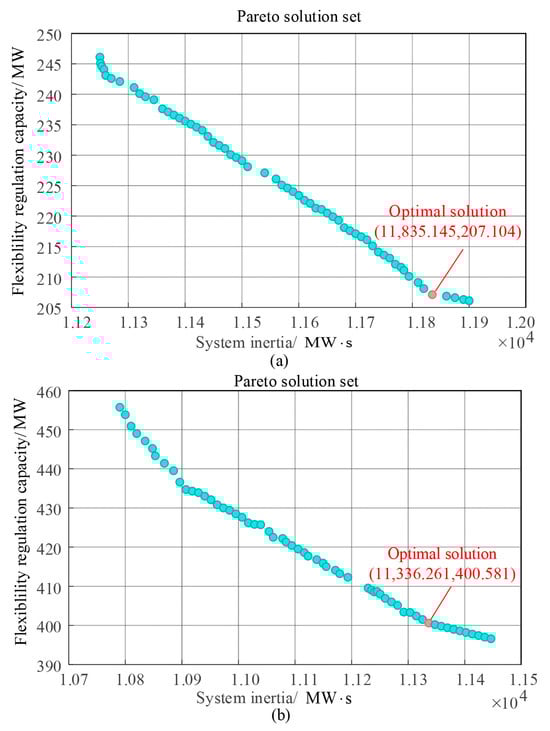
Figure 12.
The Pareto solution set of two periods in Scenario 2. (a) Pareto solution set at 15:00; (b) Pareto solution set at 20:00.
6. Conclusions
This paper proposes a system capacity requirement evaluation method for both the normal states of power balance and post-contingency frequency security. Firstly, multi-dimensional flexibility indices for the normal state are established, which can quantify the trend of supply–demand imbalance of the system under a certain generation resource mix scheme. Thermal units and electric energy storage are conducted as the benchmark flexible resources for maintaining the supply–demand balance of the system, and a normal flexible regulation capacity requirements quantitative model is established. Secondly, frequency security indices based on the frequency dynamic response of the system considering multi-type resources including SGs, renewable energy sources, and electric energy storage are derived. These indices are used to quantify the total demand for the frequency regulation capacity when maintaining frequency security after contingencies. Finally, based on the above quantitative models, a multi-objective minimum regulation capacity assessment model that takes into account the normal flexibility capacity requirements and the frequency regulation capacity requirements is proposed and solved using the NSGA-II algorithm.
The case study based on a sending-end grid with two stages shows that the proposed regulation capacity requirements assessment model can obtain the capacity required to ensure both the system power balance and frequency security under credible contingency. For a higher proportion of renewable energy (more than 45%), there exists both upward and downward regulation insufficiency during different load power demand levels. The normal and frequency regulation requirements will increase with the renewable penetration. And the frequency regulation requirements have the same trends as the system load demand. The proposed method can provide decision-making references for the power grid in terms of the construction planning of flexible resources and the arrangement of operation modes.
Author Contributions
Conceptualization, M.L., X.W. and D.C.; methodology, M.L., F.L. and Y.W.; investigation, M.L., X.W., F.L., X.G. and D.C.; writing—original draft preparation, M.L., X.W., D.C. and Y.W.; writing—review and editing, X.W., F.L. and X.G.; supervision, M.L. and Y.W.; funding acquisition, M.L., X.W., F.L. and X.G. All authors have read and agreed to the published version of the manuscript.
Funding
This research was funded by the Science and Technology Project of State Grid Sichuan Electric Power Company (Grant No. 521996230006).
Data Availability Statement
The original contributions presented in the study are included in the article, further inquiries can be directed to the corresponding author.
Conflicts of Interest
The author declares no conflicts of interest.
Nomenclature
| Abbreviations | |
| HVDC | High Voltage Direct Current |
| SG | Synchronous generators |
| WT | Wind Turbine |
| PV | Photovoltaic station |
| AC | Alternating current |
| Indices and Sets | |
| Indices of SG, WT, PV, and energy storage | |
| Indices of interval and time period of evaluation | |
| Indices of ith existing generation resources | |
| Sets of SGs, WTs, and PVs | |
| Sets of tie lines, HVDC lines, and load | |
| Parameter | |
| Power demand of load, output prediction of WT and PV | |
| Power disturbance | |
| System damping | |
| Base frequency (50 Hz) | |
| Inertial time constant of units/storage | |
| Installed capacity of units/storage | |
| Full-release time of the frequency regulation reserve | |
| Droop coefficient of SG | |
| allowable maximum frequency deviation | |
| Primary frequency regulation dead-band after a disturbance | |
| Curtailment coefficient of WT | |
| Installed capacity of WT | |
| Security threshold of maximum rate of frequency change | |
| Power output limit of thermal unit | |
| Ramp down/up limit of thermal unit | |
| Variables | |
| Upward/downward flexibility regulation | |
| Expectation of the system’s upward and downward flexibility | |
| Indicators of insufficient upward and downward flexibility | |
| Proportions of time with insufficient upward and downward flexibility | |
| Upward and downward regulation capacity requirements | |
| Output of existing generation resources | |
| Power transmitted outward through the tie lines and the HVDC lines | |
| Shedding amount load, power curtailment of WT and PV | |
| Output of benchmark thermal unit | |
| Charging and discharging power of the benchmark energy storage | |
| Equivalent inertia of the system | |
| Commitment state of SG | |
| Frequency response power of SG, WT, and energy storage | |
| Frequency regulation reserve of SG and WT and energy storage | |
| Maximum rate of frequency change | |
| Maximum frequency deviation and the corresponding time | |
| Flexible regulation capacity requirements in the normal state | |
References
- Zhao, Q.; Zhang, Y.; Zhou, X.; Chen, Z.; Yan, H.; Yang, H. A Discussion on the Flexible Regulation Capacity Requirements of China’s Power System. Engineering 2024, 33, 12–16. [Google Scholar] [CrossRef]
- Du, P.; Li, W. Frequency response impact of integration of HVDC into a low-inertia AC power grid. IEEE Trans. Power Syst. 2021, 36, 613–622. [Google Scholar] [CrossRef]
- Mohandes, B.; Moursi, M.S.E.; Hatziargyriou, N.; Khatib, S.E. A review of power system flexibility with high penetration of renewables. IEEE Trans. Power Syst. 2019, 34, 3140–3155. [Google Scholar] [CrossRef]
- Wei, W.; Chen, Y.; Wang, C.; Wu, Q.; Shahidehpour, M. Nodal flexibility requirements for tackling renewable power fluctuations. IEEE Trans. Power Syst. 2021, 36, 3227–3237. [Google Scholar] [CrossRef]
- Awadalla, M.; Bouffard, F. Flexibility Characterization of Sustainable Power Systems in Demand Space: A Data-Driven Inverse Optimization Approach. IEEE Trans. Power Syst. 2024, 39, 6196–6209. [Google Scholar] [CrossRef]
- Khatami, R.; Parvania, M.; Narayan, A. Flexibility Reserve in Power Systems: Definition and Stochastic Multi-Fidelity Optimization. IEEE Trans. Smart Grid. 2020, 11, 644–654. [Google Scholar] [CrossRef]
- Tejada-Arango, D.A.; Morales-España, G.; Wogrin, S.; Centeno, E. Power-based generation expansion planning for flexibility requirements. IEEE Trans. Power Syst. 2020, 35, 2012–2023. [Google Scholar] [CrossRef]
- Dhaliwal, N.K.; Bouffard, F.; O’Malley, M.J. A fast flexibility driven generation portfolio planning method for sustainable power systems. IEEE Trans. Sustain. Energy 2021, 12, 368–377. [Google Scholar] [CrossRef]
- Yan, K.; Li, G.; Zhang, R.; Xu, Y.; Jiang, T.; Li, X. Frequency Control and Optimal Operation of Low-Inertia Power Systems with HVDC and Renewable Energy: A Review. IEEE Trans. Power Syst. 2024, 39, 4279–4295. [Google Scholar] [CrossRef]
- Yan, R.; Masood, A.N.; Saha, K.T.; Bai, F.; Gu, H. The Anatomy of the 2016 South Australia Blackout: A Catastrophic Event in a High Renewable Network. IEEE Trans. Power Syst. 2018, 33, 5374–5388. [Google Scholar] [CrossRef]
- Ahmadi, H.; Ghasemi, H. Security-Constrained Unit Commitment with Linearized System Frequency Limit Constraints. IEEE Trans. Power Syst. 2014, 29, 1536–1545. [Google Scholar] [CrossRef]
- Jafari, M.; Gharehpetian, G.B.; Anvari-Moghaddam, A. On the Role of Virtual Inertia Units in Modern Power Systems: A Review of Control Strategies, Applications and Recent Developments. Int. J. Electr. Power Energy Syst. 2024, 159, 110067. [Google Scholar] [CrossRef]
- Paturet, M.; Markovic, U.; Delikaraoglou, S.; Vrettos, E.; Aristidou, P.; Hug, G. Stochastic Unit Commitment in Low-Inertia Grids. IEEE Trans. Power Syst. 2020, 35, 3448–3458. [Google Scholar] [CrossRef]
- Wen, Y.; Li, W.; Huang, G.; Liu, X. Frequency Dynamics Constrained Unit Commitment with Battery Energy Storage. IEEE Trans. Power Syst. 2016, 31, 5115–5125. [Google Scholar] [CrossRef]
- Li, J.; Qiao, Y.; Lu, Z.; Ma, W.; Cao, X.; Sun, R. Integrated Frequency-constrained Scheduling Considering Coordination of Frequency Regulation Capabilities from Multi-source Converters. J. Mod. Power Syst. Clean Energy 2024, 12, 261–274. [Google Scholar] [CrossRef]
- Rehman, H.U.; Yan, X.; Abdelbaky, M.A.; Jan, M.U.; Iqbal, S. An Advanced Virtual Synchronous Generator Control Technique for Frequency Regulation of Grid-Connected PV System. Int. J. Electr. Power Energy Syst. 2021, 125, 106440. [Google Scholar] [CrossRef]
- Ding, T.; Zeng, Z.; Qu, M. Two-Stage Chance-Constrained Stochastic Thermal Unit Commitment for Optimal Provision of Virtual Inertia in Wind-Storage Systems. IEEE Trans. Power Syst. 2022, 37, 4157–4167. [Google Scholar] [CrossRef]
- Shi, Z.; Xu, Y.; Wang, Y.; He, J.; Li, G.; Liu, Z. Coordinating Multiple Resources for Emergency Frequency Control in the Energy Receiving-End Power System with HVDCs. IEEE Trans. Power Syst. 2023, 38, 4708–4723. [Google Scholar] [CrossRef]
- GB/T 19963.1-2021; State Administration for Market Regulation, National Standardization Administration of China. Technical Code for Connecting Wind Farms to Power Systems—Part 1: Onshore Wind Power. China Standard Press: Beijing, China, 2021. [Google Scholar]
- Badesa, L.; Teng, F.; Strbac, G. Simultaneous scheduling of multiple frequency services in stochastic unit commitment. IEEE Trans. Power Syst. 2019, 34, 3858–3868. [Google Scholar] [CrossRef]
- Li, Y.; Kong, F.; Jing, C.; Yang, L. MILP model for peak shaving in hydro-wind-solar-storage systems with uncertainty and unit commitment. Electr. Pow. Syst. Res. 2025, 241, 111358. [Google Scholar] [CrossRef]
Disclaimer/Publisher’s Note: The statements, opinions and data contained in all publications are solely those of the individual author(s) and contributor(s) and not of MDPI and/or the editor(s). MDPI and/or the editor(s) disclaim responsibility for any injury to people or property resulting from any ideas, methods, instructions or products referred to in the content. |
© 2025 by the authors. Licensee MDPI, Basel, Switzerland. This article is an open access article distributed under the terms and conditions of the Creative Commons Attribution (CC BY) license (https://creativecommons.org/licenses/by/4.0/).