COPmax and Optimal Control of the Heat Pump Heating System Depending on the Warm Water Temperature

Abstract

The primary objective is to create a control function that ensures the energetic optimization of a heat pump heating system at any point within the On-Off regulation range. The COPmax value, the optimal performance of the circulation pump, and the actual performance of the compressor are determined based on the water temperature. The objective function is the extended COP equation of the system. The COP equation includes the efficiency of the circulation pump and the compressor. With efficiency considered, the COP is 3.057; without efficiency, it is 3.68. At discrete operating points, steady-state operation is assumed; therefore, the behavior of the components is described using algebraic equations. The equation system was solved in two cycles using numerical iterative Newton linearization and Gaussian elimination methods. First, the mass flow rate was optimized for a water temperature value, then the optimization cycle was repeated at a higher temperature. The temperature increase was 2 °C. Using the values of the optimal performance of the circulation pump and the water temperature, a polynomial control function was developed. Applying the control function, the optimal performance of the circulation pump can be calculated for any operating temperature range.

1. Introduction

Due to green policy initiatives, the adoption and application of all types of heat pumps have significantly increased across Europe in recent years. The peak was in 2022, when the number of heat pumps sold in the European Union exceeded 3 million, representing a 38% increase. Unfortunately, this trend reversed with a significant decline observed in 2024; in Germany, the number of heat pumps sold dropped by 52% [1]. This was primarily due to economic stagnation across the EU, including Germany, and as a consequence, state subsidies were reduced. However, the EU had set a target to install 10 million heat pumps by 2027 [1]. This raises the question of the energy source, the vast majority of heat pumps use electricity, with only a few exceptions operating on gas. Since both energy sources are limited, energy efficiency is essential. One modest way to improve efficiency is the optimization and control of heat pump heating systems. Naturally, such optimization efforts affect environmental protection, sustainable development, and ultimately the costs of manufacturing, maintenance, and operation.

Numerous papers have been published in leading journals on this subject. The optimization objectives in these papers vary widely: capacity, structure, control, lifetime, economic, refrigerant selection, and energy optimization. However, only a few directly address the energy optimization of heat pump heating systems, and even those do so in different ways. Liu et al. [2] established a performance optimization method for an air-source heat pump heating system. Their optimization achieved a 33% reduction in heat pump performance at a design point temperature of 22 °C, along with a reduction in CO₂ emissions. Pesola A. [3] designed a cost-optimization model for a district heating system with decentralized heat pumps. Optimal utilization of heating components reduced average operational expenditure by 24%. Masternak C. et al. [4] developed an interdisciplinary model for the optimal sizing of heat pumps. The goal was to minimize both cost and CO₂ emissions. Their optimization resulted in a 3.1-fold reduction in life-cycle CO₂ emissions, based on Belgian thermally insulated dwellings. Brida V. Mbuwir et al. [5] presented the results of a model predictive control approach to optimize the operation of a multi-source heat pump system for space heating and domestic hot water. Their objective was to minimize electricity consumption. Using BEMS control, electricity usage was reduced by approximately 7% compared to conventional on/off control. A key challenge in this predictive control approach is developing accurate white-box models for system components. Hosseinnia M. S. et al. [6] focused on the techno-economic optimization of a solar-assisted ground source heat pump. They analyzed the total annual cost and optimized the system design, using a 200 m vertical ground heat exchanger. Electricity consumption was reduced by 55.9% in September and 79.2% in March. The study by Granryd E. [7] is perhaps the most closely related to our research topic. The system structure and research objective were similar, although Granryd examined an air-to-air heat pump, optimizing the air mass flow rate through the fan. The mathematical method used was analytical, with many approximations and the assumption of an ideal refrigeration cycle, which differs from real-world processes. The system’s COP was the objective function, but with significant simplifications. In contrast, we studied a water-to-water heat pump using a real refrigeration cycle, including the compressor and circulation pump efficiencies and a condenser model that includes both desuperheating and condensation phases. We applied a numerical method, which allowed for greater complexity in the mathematical model and better graphical representation of the results. Cervera-Vázquez J. et al. [8] applied a situ optimization methodology based on pump frequency variation in a heat pump system with two compressors and on/off control. During compressor operation, the pump frequency varies depending on whether compressors run singly or in parallel. Using this optimization method, energy savings of up to 32% were achieved. The article by Edwards K. C. et al. [9] is practically a continuation of [8]. The system is the same, a two-compressor heating and cooling heat pump with external and internal water pumps. The difference is that in [9], pump frequency optimization is applied throughout the entire heating season, resulting in 30–40% energy savings. In our study, the system uses a single compressor, and the optimal performance control of the circulation pump is based on feedback from the water temperature. The circulation pump’s optimal performance is achieved by adjusting its frequency, i.e., rotational speed.

The topics of the studies above are expanded, so this paper aims to examine the internal energy optimums of heat pump heating systems. The ultimate objective is to analyze the energy components and COP as functions of the varying water temperature during operation, and to derive a control function accordingly. Heat pump systems, including water-to-water, air-to-air, and air-to-water types, have nine degrees of freedom [10] of which only three are energy-related: two local and one global. One local optimum is the energy optimum of the warm water circuit, the other is the cold-water circuit, and the global optimum is the simultaneous optimization of both. In this case study, we focus on the energy optimization and control of the warm water circuit in a water-to-water heat pump system.

The type [11,12] and heating performance of the heat pump are selected based on the building’s energy demands. Following this, it is necessary to determine the appropriate performance for pumps and possibly fans. Although several design methods exist, none one ensures optimal pump performance. Energy efficiency, however, is an increasingly important factor in operating systems, including heat pump systems [13,14]. Therefore, this paper presents a numerical optimization method and its application in a case study. As a result, we identify and analyze the optimal performance of the circulation pump for a given water temperature, and then as a function of varying water temperatures. Regardless of control type during heat pump operation, the water temperature continuously rises, posing a challenge to examine how energy components behave at different operating points depending on temperature. For this purpose, we used an existing optimization algorithm Nyers, A. et al. [15], expanded with a new independent variable, water temperature. As a function of this temperature, the following were determined: the control function of the circulation pump, the COP of the heating system, the real performance of the compressor, the heat flow, and the optimal real performance of the circulation pump.

The control function of the circulation pump allows its optimal operation at all operating points, depending on the varying water temperature. Most water-to-water heat pumps use On-Off control, causing the water temperature to increase during operation, typically between 30 and 60 °C. Consequently, the circulation pump’s optimal performance also has to change. Applying the control function, the optimal performance can be calculated based on the current water temperature. The microprocessor controller of the Willo pump ensures optimal pump performance by adjusting speed, thereby maximizing the COP at all operating points.

The operation of a water-to-water heat pump heating system is slightly non-stationary. Under On-Off control strategies, the water temperature gradually increases, depending on heater type, external temperature, and controller accuracy. The source water temperature may also vary slightly. In dual-well systems, the source temperature remains practically constant during operation (around 14 °C at 40 m depth), though the cooling water temperature may rise slightly (by 2–4 °C), reducing COP.

The base heating system model is time-independent, with lumped parameters, algebraic, coupled, nonlinear, and composed of many equations. It includes algebraic equations for refrigerant R134a, COP, condenser, compressor, and circulation pump performance.

Optimization can be performed using analytical or numerical methods. Analytical methods require a high level of mathematical expertise and are only applicable up to a certain point; further analysis must rely on numerical techniques. With numerical methods, obtaining results is somewhat easier, especially since the MATLAB 2015a software package [16] includes solver programs. These solver programs, however, act as black boxes, which can obscure the physical interpretation of the mathematical model.

After all, a discrete optimization approach was chosen instead of continuous-time integration. The discrete method is favorable for the numerical procedure. The change in the thermal systems is slow and uniform, without jumping, so that the tendency of change is drawn by connecting a small number of discrete points. In the initial step, a discrete temperature value was considered, assuming the steady-state operating mode at the working point. Therefore, in the mathematical model, the equations were not differential but algebraic. In the second step, the model and the program were expanded with a new variable, namely water temperature. The diagrams drawn using optimization values are smooth, and consequently, simulations can be done with higher temperature increments.

The coefficient of performance (COP) is the objective function for the optimization procedure [17,18]. Its equation with the efficiencies of the circulation pump and compressor is extended. The equations for heat flows, performance expressions, and efficiencies all depend on the water’s mass flow and inlet temperature. Such a complex system of equations is best solved numerically using, for example, Newton linearization and Gaussian elimination. The model’s solution program is part of MATLAB 2015a.

The research on analytical-numerical energy optimization and control of heat pump heating and cooling systems can be continued. Future case studies will address the combined energy optimization and control of warm and cold water circuits.

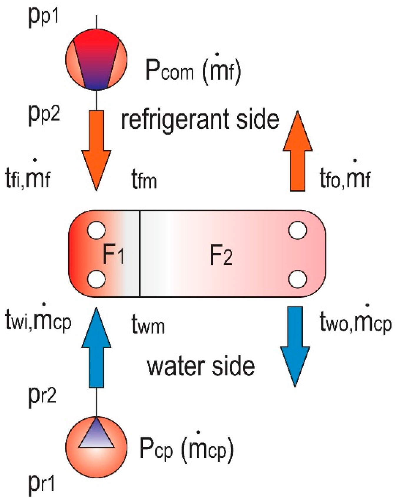
2. Physical Model of the Hot Water Circuit

The active energy elements of the warm water circuit are the condenser, the compressor, the circulation pump, and the heating surfaces. In this case, the well pump is a passive participant, and its performance is variable-constant.

The operation of the hot water circuit is well-known. In the examined case, in the plate heat exchanger, the high-temperature vapor delivered by the compressor transfers its heat to the water, causing it to condense. The water flows, using the energy provided by the circulation pump, and delivers the heat to the heating surfaces. The purpose of Figure 1 is to illustrate and indicate the heat flows, performance outputs, and variables occurring in the water and refrigeration circuit.

3. Mathematical Methods

3.1. Description of the Aim

The goal of the case study is also the energy optimization and control of the heating system. Within this framework, the following were determined: the optimal control function, the maximum of the coefficient of performance, and the optimal performance of the circulation pump as a function of the wate temperature.

3.2. Objective Functions of the Heat Pump Heating System—COP

The coefficient of performance related to the condenser circuit serves as the objective function of the optimization procedure. Some terms in the COP equation are functions of the hot water mass flow rate, and all terms are functions of the water temperature, $t_{wi}.$ The real performance of the well pump is independent of the warem water temperature and is treated as a variable constant.

The basic numerical procedure determines the optimal value of the mass flow rate for a given water temperature. Using the optimal mass flow rate, the optimal performance of the circulation pump and the maximum COP can be determined. In the study, the program was extended to cover changes in water temperature in the range of 30–55 °C. As a result, the maximum COP and the optimal performance of the circulation pump can be determined for each value of the varying water temperature.

The COP equation includes the efficiency of the circulation pump and the compressor, which significantly affects the value of the COP.

$$CO{P}_{max}\left({\dot{m}}_{cp,opt},t_{wi}\right)=\left|\right|{{\displaystyle \frac{q\left({\dot{m}}_{cp,opt},t_{wi}\right)+ P_{cp,e}\left({\dot{m}}_{cp,opt},t_{wi}\right)}{\frac{P_{com,r}\left({\dot{m}}_{cp,opt},t_{wi}\right)}{{\eta }_{com}\left(P_{com,r}\right)}+P_{wp,r} +\frac{P_{cp,e}\left({\dot{m}}_{cp,opt},t_{wi}\right)}{{\eta }_{cp}\left({\dot{m}}_{cp,opt},t_{wi}\right)}}}\left|\right|}_{max}$$

(1)

3.3. Mathematical Model of the Condenser

According to its operation, the condenser consists of the vapor cooling section and the condensation section. Therefore, its base model is divided into two parts, and includes the heat flow equations, $q_1$ and $q_2$, and numerous auxiliary equations [19]. The heat flow $q_1$ is realized on surface $F_1$, and $q_2$ on surface $F_2$. The total heat flow $q$ is the sum of $q_1$ and $q_2$. The effective surface of the condenser, denoted $F$, is the sum of the surfaces $F_1$ and $F_2$.

The modified equations of the condenser [19].

In the vapor cooling section, the heat flow is.

$$q_1=\left(F-{\displaystyle \frac{q_2}{k_{f2}·\Delta t_{ln2}}}\right)·k_{f1}·\Delta t_{ln1}$$

(2)

In the vapor condensation section, the heat flow is.

$$q_2={\dot{m}}_f·\left(a_o+a_1·\left(-{\displaystyle \frac{{\mathrm{q}}_1}{C_{pf}·{\dot{m}}_f}}+t_{fi}\right)+a_2·{\left(-{\displaystyle \frac{{\mathrm{q}}_1}{C_{pf}·{\dot{m}}_f}}+t_{fi}\right)}^2\right)$$

(3)

In the condensation section, the heat flow equation is the latent heat equation in polynomial form. The equations are coupled and can only be solved by iterative numerical methods.

Auxiliary Equations

The logarithmic temperature difference of the condenser’s vapor cooling and condensation sections was approximated to the arithmetic. The difference between the logarithmic and arithmetic temperature is only 0.2% [19].

The arithmetic temperature difference of the vapor cooling section.

$$\Delta t_{ln1}\cong 0.5·\left(\left(t_{fi}-t_{wi}\right)+\left(t_{fm}-t_{wm}\right)\right)$$

(4)

The arithmetic temperature difference of the condenser vapor condensation section.

$$\Delta {\mathrm{t}}_{\ln 2}\cong 0.5·\left(\left({\mathrm{t}}_{\mathrm{fm}}-{\mathrm{t}}_{\mathrm{wm}}\right)+\left({\mathrm{t}}_{\mathrm{fo}}-{\mathrm{t}}_{\mathrm{wo}}\right)\right)$$

(5)

The heat transfer coefficient is approximated [20]:

$$k_{1,2}\cong {\displaystyle \frac{{\alpha }_w·{\alpha }_{f1,2}}{{\alpha }_w+{\alpha }_{f1,2}}}$$

(6)

1. Vapor cooling section, 2. condensation section.

The heat transfer coefficient was determined approximately. Namely, the wall thickness of the heat exchanger is (0.3–0.5) mm, therefore, the term δ/λ ≅ 0 in the equation is approximately zero. The heat transfer coefficient of water is the same in the cooling and condensation sections.

3.4. Mathematical Model of the Circulation Pump

The effective performance model of the circulation pump is lumped and independent of time:

$$P_{cp,e}={\displaystyle \frac{{{\dot{m}}_{cp}}^3}{{{\rho }_w}^2}}·{{\displaystyle \sum }}_1^n{k}_{pi}$$

(7)

The pressure drop in the pipeline is a function of the water mass flow rate, according to the Darcy–Weisbach equation. The $k_{pi}$ coefficient takes into account the geometry of the pipeline system. In the case of a system with a known structure, its value is approximately constant. However, the Reynolds number, Re depends slightly on the mass flow rate, with an exponent of 0.75. Nevertheless, the Reynolds number should also be incorporated into the numerical simulation.

$$k_{pi}=\left({{\displaystyle \sum }}_{i=1}^n{\xi }_i\left(Re, \epsilon \right)·{\displaystyle \frac{l_i}{d_i}}+{{\displaystyle \sum }}_{i=1}^n{\xi }_{i,lok}\left(goem\right)\right)·{\displaystyle \frac{1}{{2·A_d}^2}}\cong const.$$

(8)

Determining the real pump performance, energy dissipation is taken into account using the pump efficiency. The efficiency is determined based on measured values from the real pump. Using the measured real and effective pump performance values, the efficiencies were calculated, and the ${\eta }_{cp}$ − $P_{cp,e}$ polynomial was established [15,18].

$$P_{cp,r}\left({\dot{m}}_{cp}\right)={\displaystyle \frac{P_{cp,e}}{ {\eta }_{cp}\left({\dot{m}}_{cp}\left(P_{cp,e}\right)\right)}}={\displaystyle \frac{P_{cp,e}}{ a_o+a_1·P_{cp,e}+a_2·{P_{cp,e}}^2+\cdots }}$$

(9)

3.5. Mathematical Model of the Compressor

In the procedure, when determining the optimal performance of the circulation pump, the real performance of the compressor is variable constant. In calculating the real performance of the compressor, the efficiency ${\eta }_{com}\left(P_{com,r}\right)$ was taken into account. This efficiency was calculated based on the measured real and the computed effective performance values. Using these data pairs and the MATLAB 2015a software package, a polynomial was created as a function of the real performance [15].

$$P_{com,e}=P_{com,r}·{\eta }_{com}\left(P_{com,r}\right)=P_{com,r}·\left(a_o+a_1·P_{com,r}+a_2·{P_{com,r}}^2+\cdots \right)$$

(10)

The effective performance of the compressor can be used to determine the mass flow rate of the refrigerant and the vapor temperature at the compressor outlet. The refrigerant mass flow rate is determined using the enthalpy increase due to compression and the effective performance consumed by the compressor.

$${\dot{m}}_f=P_{com,e}·{\left(i_{f,i}-i_{f,e}\right)}^{-1}$$

(11)

The vapor temperature at the compressor outlet can be calculated using the enthalpy increase and the effective performance of the compressor:

$$P_{com,e} \cong {\dot{m}}_f·C_{p,f,com}· \left(t_{f,i} -t_{f,e}\right)$$

(12)

The average specific heat of the vapor during compression, $C_{p,f,com}$, can be estimated using a linear approximation. It is equal to the average of the inlet specific heat $C_{p,f }\left(t_{f,i}\right)$, and the outlet specific heat $C_{p,f}\left(t_{f,e}\right)$ [15].

Finally, the vapor temperature at the compressor outlet can also be expressed, based on Equation (12), as:

$$t_{f,i}\cong {\displaystyle \frac{P_{com,e} }{{\dot{m}}_f·C_{p,f, com}}}+t_{f,e}$$

(13)

4. Control Function

In the case of On/Off control, the algorithm of the control function is activated when the heat pump heating system starts. The control adjusts the circulation pump’s performance and speed to optimal values, based on the current value of the water temperature $t_{w,i}$.

Physically, the temperature varies continuously, so optimal control must also be continuous. Therefore, the control function must be continuous as well. In the On-Off domain, ensuring continuity mathematically means integrating the control function as a function of the water temperature. The challenge is that the optimal control function depends on the mass flow rate and the water temperature, making its integration difficult. However, a semi-continuous discrete function is much easier to define. Instead of integration, a numerical discrete method can be applied.

The strategy is to optimize all variables for an initial given water temperature in the first cycle. In the next cycle, all variables: the optimal water mass flow rate, optimal circulation pump performance, COPmax, compressor performance, and heat flow were calculated depending on a discretely increased water temperature. The temperature increment is ∆$t_{w,i}$ = 2 °C. Applying the optimal performance and temperature value pairs a continuous control function was created in polynomial form in the MATLAB 2015a program.

The integrated form of the continuous control function of the circulation pump’s optimal performance.

$$P_{cp,r,opt}\left({\dot{m}}_{cp,opt}\left(t_{w,i}\right),t_{w,i}\right)={{\displaystyle \int }}_{t_{w,i,on}}^{t_{w,i,off}}f\left(P_{cp,r,opt}\left({\dot{m}}_{cp,opt}\left(t_{w,i}\right),t_{w,i}\right)\right)·d{t}_{w,i}$$

(14)

Cycle of increasing water temperature.

$$\begin{gathered} j=1: t_{w,i,j}=t_{w,i,o}, \Delta t_{w,i}=0 \\ j=2: t_{w,i,j}=t_{w,i,j}+\Delta t_{w,i}, \end{gathered}$$

(15)

In each operating point (i.e., for each water temperature in the ‘$\mathrm{j}$’ cycle), the optimal water mass flow rate, optimal circulation pump performance, and COP maximum are calculated.

$$j=1÷n t_{w,i,j}=const, \to {\dot{m}}_{cp,opt,j},\left(t_{w,i,j}\right)=opt. \to P_{cp,r,j,opt}\left({\dot{m}}_{cp,opt}\left(t_{w,i,j}\right), t_{w,i,j}\right)$$

(16)

The circulation pump’s optimal performance as a function of the water temperature.

$$P_{cp,r,j,opt}\left({\dot{m}}_{cp,opt,j}\left(t_{w,i,j}\right), t_{w,i,j}\right)\cong a_o+a_1·t_{w,i,j}+a_2·{t_{w,i,j}}^2+\cdots j=1\dots n$$

(17)

“$\mathrm{j}$” is the sampling number of water temperature.

The numerical controller, using feedback, samples the water temperature ‘j’ times with the help of the sensor, and by applying the control function, calculates the optimal pump performance and the optimal pump speed for each operating point.

Circulation pump optimal speed depand on the optimal pump performance and the torque of the electro motor.

$$n_{cp,r,j,opt}\left({\dot{m}}_{cp,j,opt}\left(t_{w,i,j}\right), t_{w,i,j}\right)={\displaystyle \frac{P_{cp,r,opt}\left({\dot{m}}_{cp,opt,j}\left(t_{w,i,j}\right), t_{w,i,j}\right)}{M_{cp,r}\left(n_{cp,r,j,opt}\right)}}$$

(18)

5. Numerical Procedure

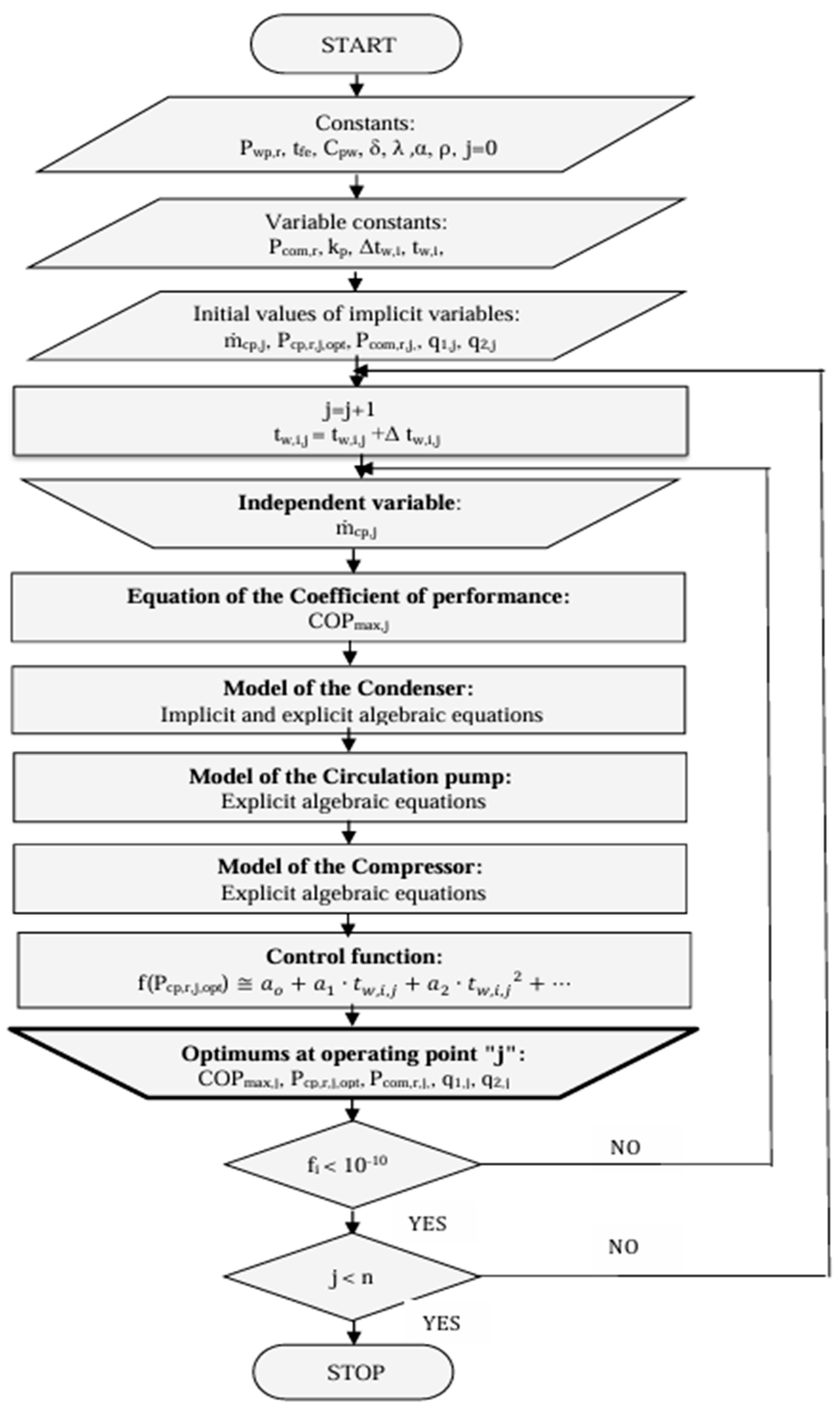
The mathematical model of the heating system consists of a lumped, coupled and a large number of nonlinear algebraic equations. This system of equations can be solved numerically, using Newton linearization and Gauss elimination methods [16]. The algorithm is iterative, because most of the algebraic equations are implicit, so the initial values of the unknown variables must be assumed. Experience has shown that the proposed values must be close to the solution; otherwise, the initial iteration will not converge.

In the numerical optimization procedure, the objective function is the Coefficient of Performance (COP) of the heating system. In the analytical method, the condition for the optimum is that the first derivative of COP with respect to the water mass flow rate equals zero. In the numerical method, no exact optimality condition equation; instead, the water mass flow rate varies at discrete points within an arbitrary domain in the simulation. The COP and other dependent variables are calculated at these discrete points. The maximum value in the resulting COP sequence at the discrete points is the extremum, i.e., the energy optimum COP_max. The water mass flow rate corresponding to the maximum COP is the optimal mass flow rate.

Three energetic components operate in the water circuit: two pumps and a compressor. This study focuses on one of the local optimum. The circulation pump performance should be optimized depending on the water temperature. By the simulation, the compressor performance is variable, while the well pump performance is constant.

The input parameters of the algorithm: the active surface area of the plate condenser, the constant physical characteristics of water, and refrigerant. The input temperatures of the water and the refrigerant ($t_{w,i}$ and $t_{f,e}$) are variable constants. Figure 2.

The basic numerical optimization method yields discrete results; it provides the optimal water mass flow rate for discrete water temperatures. Based on this value, the optimal performance of the circulation pump, its efficiency, and the maximum coefficient of performance can be calculated. In the system of equations, the water temperature twi is an increasing independent variable and appears in the heat flow equations $q_1$ and $q_2$. Its variation indirectly affects the values of other system parameters as well.

However, the ultimate goal of the analysis is to investigate the optimum of the heating system not only at one water temperature but across the entire examined domain of water temperature increments.

As mentioned earlier, during the operation of the heat pump heating system, the water temperature increases; therefore, it is advisable to perform the optimization simulation for various input water temperatures: $t_{w,i}$ = (30, 35, 40, 45, 50, 55, 60) °C. The optimal mass flow rates were calculated at these discrete water temperatures, and based on the calculated values, the optimal performances of the circulation pump, the maximum coefficient of performance values COP_max,i, compressor performances, and the resulting heat flows were determined.

Applying the MATLAB 2015a software package and values of the optimal performance of the circulation pump obtained through simulation, as well as the discrete values of water temperatures, a polynomial control function was created. Applying the control function and the measured instantaneous water temperature during operation, the COPmax and optimal circulation pump performance can be calculated at every discrete temperature value in the operating heating system.

Figure 2. Algorithm for the creation of the control function based on energy optimization.

Figure 2. Algorithm for the creation of the control function based on energy optimization.

• Constants:
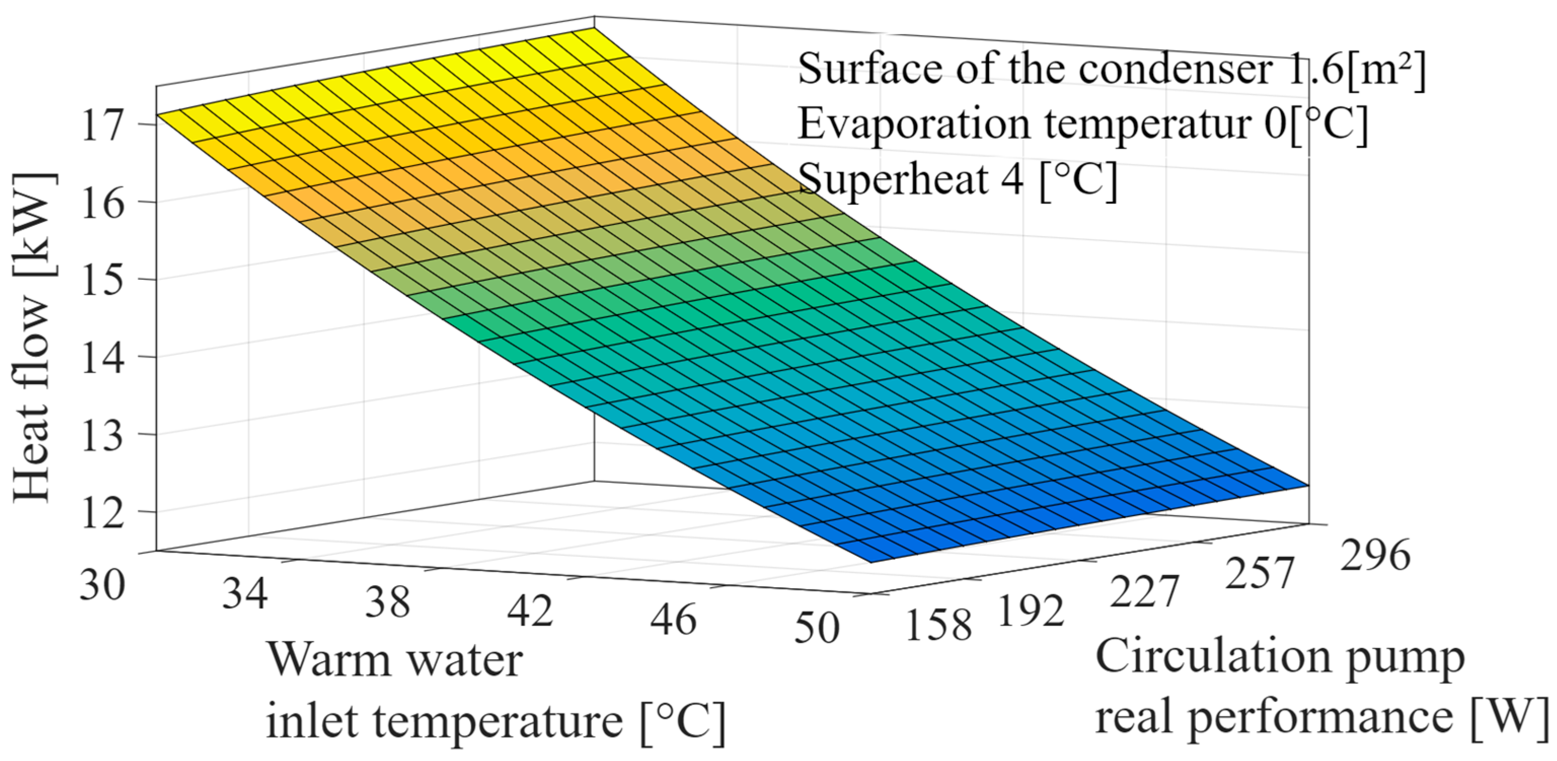
  • Nominal and effective surface area of the plate condenser: F = 2 [m²] and 1.6 [m²]
  • Real performance of the well pump: P_wp,r = 505 [W]
  • Water dencity ${\rho }_w=1000\left[{\displaystyle \frac{\mathrm{kg}}{{\mathrm{m}}^3}}\right]$
• Input Independent variable constants:
  • Discrete water temperatures at the condenser inlet:
    $t_{w,i }$ = (30, 35, 40, 45, 50, 55, 60) [°C]
  • Refrigerant vapor temperature at the compressor inlet: $t_{f,e }$ = 4 [°C]
• Output Dependent Variables:
  • Maximum value of the system’s Coefficient of Performance, COP_max
  • Optimal real performance of the circulation pump, P_cp,r,opt
  • Efficiency of the circulation pump
  • Real performance demand of the compressor, P_com,r
  • Efficiency of the compressor
  • Optimal water mass flow rates, ṁ_cp,opt
  • Control function of the optimal circulation pump performance

6. Results and Discussion

Within the framework of the optimization procedure, the effect of the efficiency of the circulation pump on the COP value was investigated.

The COP values shown in the diagram, Figure 3, the circulation pump efficiency was not taken into account during the calculation, therefore the COP value is 3.385, 9.8% higher than the real value. Namely, based on the simulation and measurements, the real COP value ranges between 3.057–3.058.

Without considering these efficiencies, the COP is 3.38, whereas including them reduces it to 3.077, a difference of 9.8% (see Figure 4).

The analytical simulation is the result of the previous research. The COP value obtained with the analytical and numerical simulation shows an insignificant difference.

A slight extreme can be observed at all temperature values on the 3D grid. At the extreme point, the COP is maximum, and the circulation pump performance is optimum. COP_max = 3.057 and P_cp,r,opt = 230 W at $t_{w,i}$ = 40 °C.

When sizing and selecting the circulation pump, it is worth going only to the optimal performance value. In a given case, this range is 158–236 W in this range, the COP value hardly changes. Therefore, a lower-performance, cheaper circulation pump is suitable financially and energetically as well.

The circulation pump’s performance is higher at 30 °C than at 50 °C water temperatures, so its effect on COPmax is more intense.

The heat flow value increases slightly with the increase in the circulation pump performance and decreases significantly with the increase in the inlet water temperature, but without extrem, see Figure 5. The COP and heat flow diagram show a similarity. It is understandable, since the heat flow value dominates among the terms in the COP equation. Its average value is about 4 times higher than the compressor power, 6 times higher than the well pump performance, and 12 times higher than the circulation pump power value.

After optimizing the circulation pump performance according to warm water temperature, using its values, the control function was created (17). Applying the control function at every temperature value enables the computation of the optimum performance. Using Equation (17), the function’s graph was drawn. On the graph, Figure 6. the circulation pump performance is optimum at every temperature value.

The optimum of the circulation pump performance exponentially decreases if the water inlet temperature increases.

It is worth analyzing how the performance of each energy component affects the energy optimum and its indicator, the COP. In the heating system examined in the case study, the optimal performance of the circulation pump at 40 °C heating water temperature is 230 W, the well pump’s is 505 W, and the compressor’s is 4050 W. The ratios are: 505:230 = 2.2, 4050:230 = 17.6, and 4050:505 = 8.02. These values show that the compressor’s performance is dominant, 17.6 times higher than the circulation pump. Consequently, the circulation pump has an optimal performance value, nevertheless, its effect on the COP is slight.

7. Conclusions

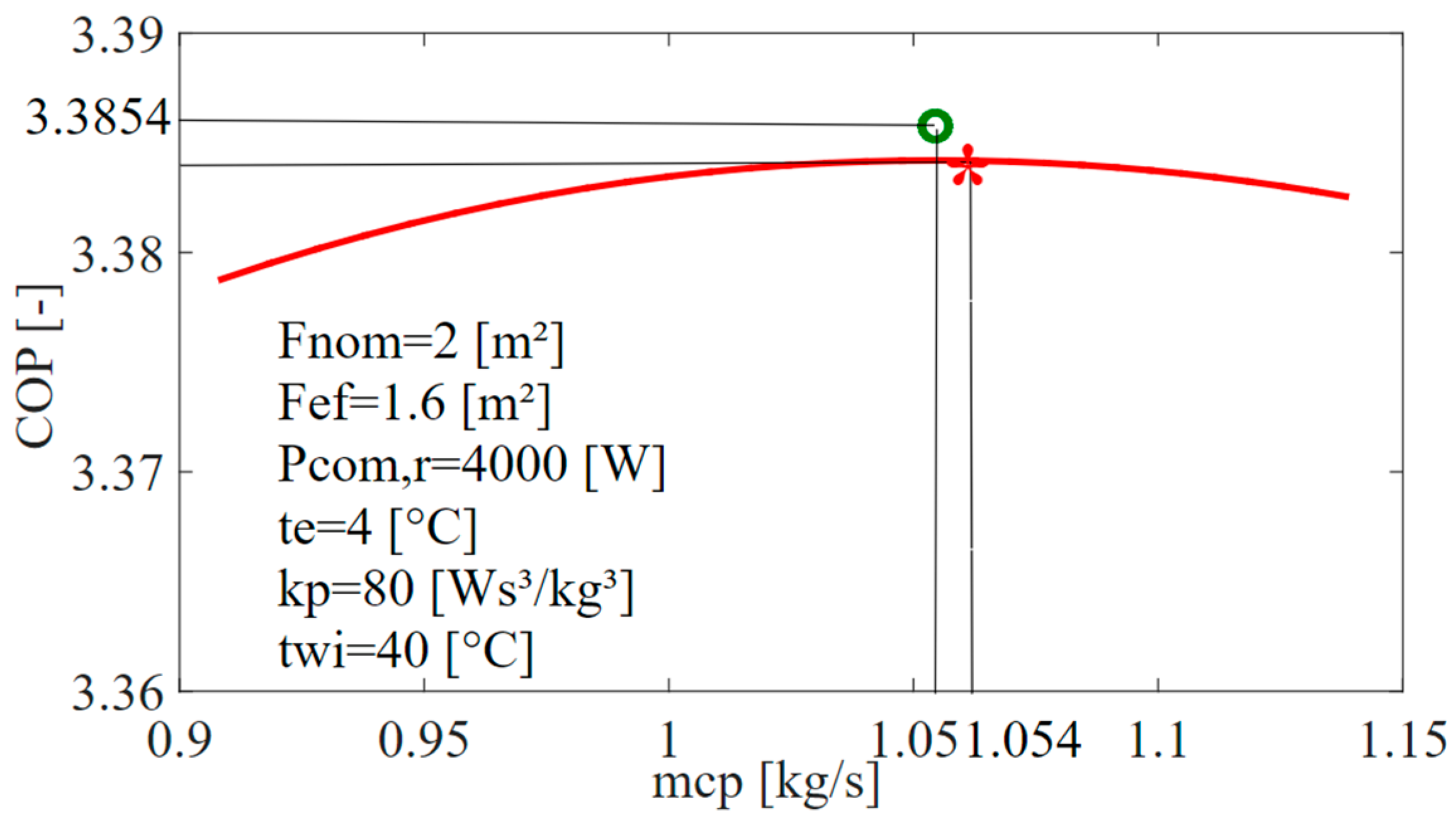
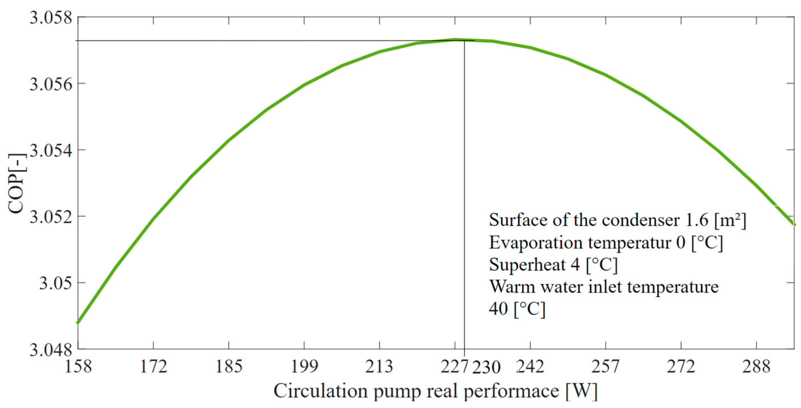
• The efficiency of the optimization-based control system is most perceptible in high-capacity heating systems. In smaller systems, optimization results in only a few tenths of a percent. In this case study, the COP increase using optimal control is only 0.03%, see Figure 7. The COP increase applies to the optimal performance of the circulation pump in the range of 158–230 W.
• In the case study, the effect of the optimized circulation pump on the COP is slight (see Figure 4 and Figure 7). The COP around the optimum varies only slightly, which means a near-optimal pump performance can be selected over a wide performance range.
• When selecting the circulation pump, it is only worthwhile to consider the real performance value up to the optimal range, between 158 W and 230 W. Although higher-performance pumps are available, they are more expensive and negatively affect the COP.
• In piping systems with higher hydraulic resistance, expedient to apply an optimized control strategy, because the circulation pump requires larger performance, see (7) and (8), which impacts the maximum COP increases (1).
• Since heating systems differ in the size of the compressor, piping, and heat exchanger, the coefficients a1, a2, and a3 used in the control function must be redefined for each system.
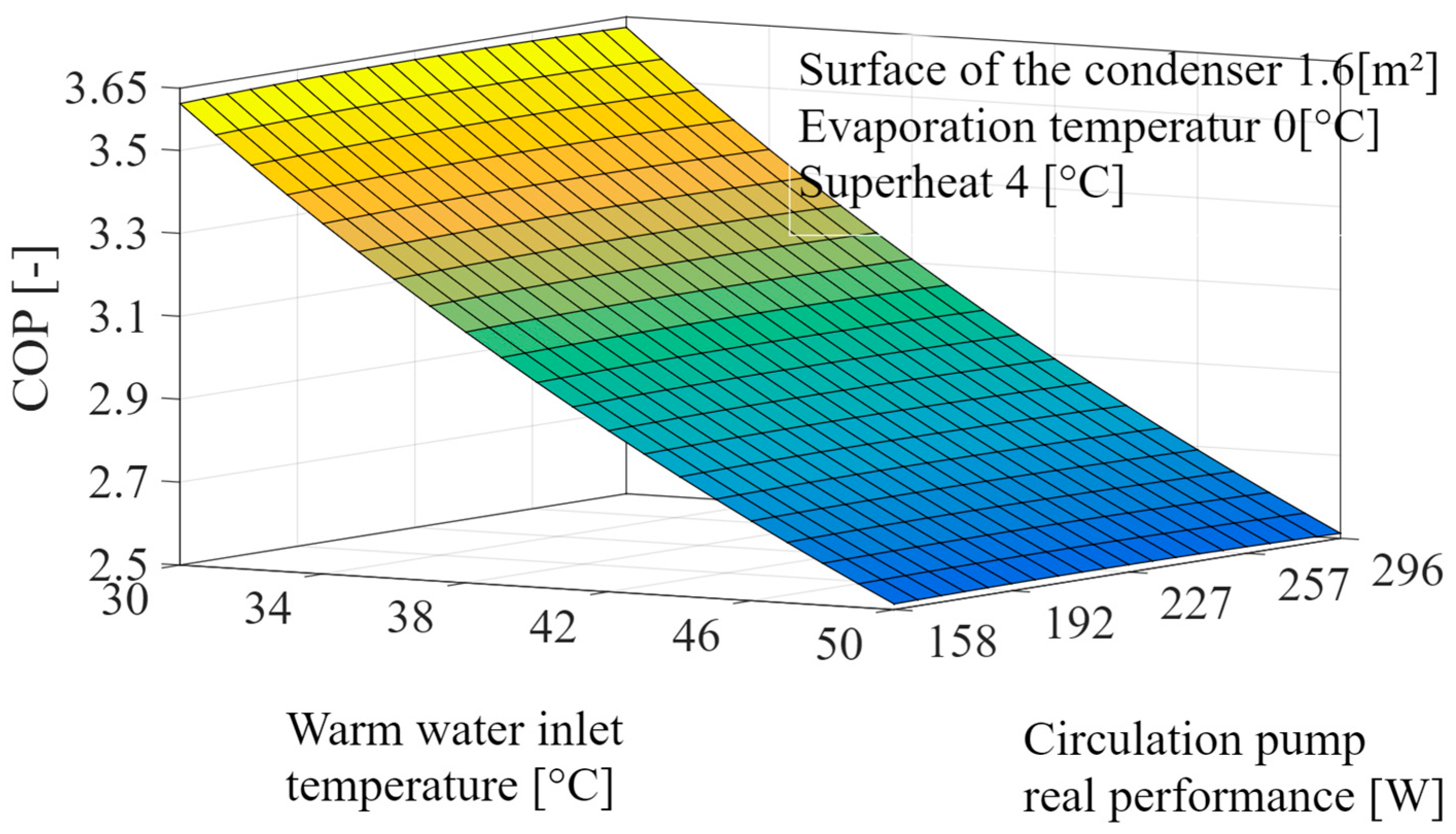
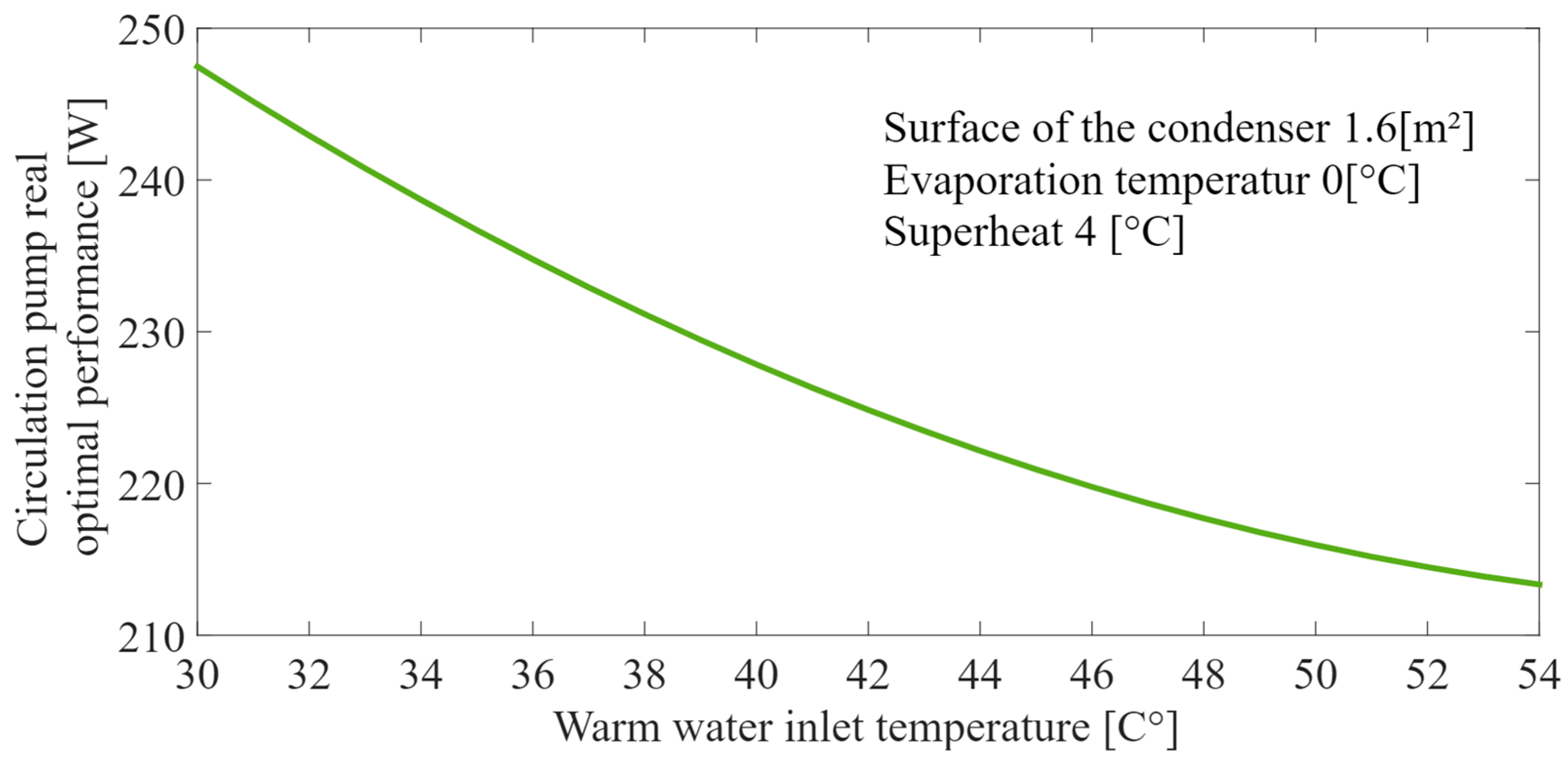
• Greater energy savings can be achieved when the circulation pump operates optimally across the entire heating water temperature range, see Figure 4.
• The performance of each energy component affects the energy optimum and its indicator, the COP. For example, the compressor performance is 17.6 times higher than that of the circulation pump. Therefore, the effect of the optimal performance of the circulation pump on the COP is small.
• Additionally, in the COP equation, the circulation pump’s effective performance appears in the numerator, but its real performance appears in the denominator. This is another reason why the circulation pump’s effect on the COP and the energy optimum is slight, see (1).
• The well pump’s expected impact on the COP and the energy optimum is several times greater than that of the circulation pump. Its performance is 2.2 times greater than the circulation pump and only 8.02 times lower than the compressor performance. Furthermore, its real performance appears only in the denominator of the COP equation. Therefore, a significant improvement in the energy efficiency of the heating system is expected if the well pump’s performance is optimized, see (1).
• A considerable increase in energy efficiency is expected through the simultaneous optimization of the well pump and the circulation pump performance. This will be the focus of our next research, applying the same optimization method.

References

1. Mindenki hőszivattyút akar venni, nincs is már elég a piacon. Magyar Hőszivattyú Szövetség. Budapest, Konferencia. 2022. Available online: https://www.vg.hu/energia-vgplus/2023/04/mindenki-hoszivattyut-akar-venni-nincs-is-mar-eleg (accessed on 1 July 2025).
2. Liu, Z.; He, M.; Tang, X.; Yuan, G.; Yang, B.; Yu, X.; Wang, Z. Capacity optimisation and multi-dimensional analysis of air-source heat pump heating system: A case study. Energy 2024, 294, 130784. [Google Scholar] [CrossRef]
3. Pesola, A. Cost-optimization model to design and operate hybrid heating systems–Case study of district heating system with decentralized heat pumps. Energy 2023, 281, 128241. [Google Scholar] [CrossRef]
4. Masternak, C.; Reinbold, V.; Meunier, S.; Saelens, D.; Marchand, C. Heat pumps optimal sizing and operation accounting for techno-economic and environmental aspects. Energy Build. 2024, 325, 114904. [Google Scholar] [CrossRef]
5. Mbuwir, B.V.; Geysen, D.; Kosmadakis, G.; Pilou, M.; Meramveliotakis, G.; Toersche, H. Optimal control of a heat pump-based energy system for space heating and hot water provision in buildings: Results from a field test. Energy Build. 2024, 310, 114116. [Google Scholar] [CrossRef]
6. Hosseinnia, M.S.; Sorin, M. Techno-economic approach for optimum solar assisted ground source heat pump integration in buildings. Energy Convers. Manag. 2022, 267, 115947. [Google Scholar] [CrossRef]
7. Granryd, E. Analytical expressions for optimum flow rates in evaporators and condensers of heat pumping systems. Int. J. Refrig. 2010, 33, 1211–1220. [Google Scholar] [CrossRef]
8. Cervera-Vázquez, J.; Montagud, C.; Corberán, J.M. In situ optimization methodology for the water circulation pumps frequency of ground source heat pump systems: Analysis for multistage heat pump units. Energy Build. 2015, 88, 238–247. [Google Scholar] [CrossRef]
9. Edwards, K.C.; Finn, D.P. Generalized water flow rate control strategy for optimal part load operation of ground source heat pump systems. Appl. Energy 2015, 150, 50–60. [Google Scholar] [CrossRef]
10. Jensen, B.J.; Skogestad, S. Degrees of freedom and optimality of sub-cooling. Comput. Chem. Eng. 2007, 31, 712–721. [Google Scholar] [CrossRef]
11. Meng, X.; Zhou, X.; Li, Z. Review of the Coupled System of Solar and Air Source Heat Pump. Energies 2024, 17, 6045. [Google Scholar] [CrossRef]
12. Lai, Y.; Gao, Y.; Gao, Y. Impact of Energy System Optimization Based on Different Ground Source Heat Pump Models. Energies 2024, 17, 6023. [Google Scholar] [CrossRef]
13. Ciuman, P.; Kaczmarczyk, J.; Winnicka-Jasłowska, D. Investigation of Energy-Efficient Solutions for Single-Family House Based on the 4E Idea in Poland. Energies 2025, 18, 449. [Google Scholar] [CrossRef]
14. Eordoghne Miklos, M. Investigation of energy efficiency of pumping systems by a newly specified energy parameter. In Proceedings of the 11th International Symposium on Exploitation of Renewable Energy Sources and Efficiency, Proceedings EXPRES, Subotica, Serbia, 11–13 April 2019; pp. 21–25, ISBN 978-86-919769-4-1. [Google Scholar]
15. Nyers, A.; Nyers, J. Enhancing the Energy Efficiency—COP of the Heat Pump Heating System by Energy Optimization and a Case Study. Energies 2023, 16, 2981. [Google Scholar] [CrossRef]
16. MATLAB 2015a Software Package. Available online: https://www.mathworks.com/matlabcentral/answers/433589-how-to-download-matlab-2015a#accepted_answer_350303 (accessed on 1 July 2025).
17. Santa, R.; Garbai, L.; Fürstner, I. Optimization of heat pump system. Energy 2015, 89, 45–54. [Google Scholar] [CrossRef]
18. Atasoy, E.; Çetin, B.; Bayer, O. Experiment-based optimization of an energy-efficient heat pump integrated water heater for household appliances. Energy 2022, 245, 123308. [Google Scholar] [CrossRef]
19. MATLAB Programming and Numeric Computing Platform. Available online: https://www.mathworks.com/products/matlab (accessed on 1 July 2025).
20. Astina, M.I.; Sato, H. A fundamental equation of state for 1,1,1,2-tetrafluoroethane with an intermolecular potential energy background and reliable ideal-gas properties. Fluid Phase Equilibria 2004, 221, 103–111. [Google Scholar] [CrossRef]
Figure 1. Condenser warm water circuit of the heat pump heating system. 1 is the vapor cooling section, 2 is the vapor condensation section.
Energies 18 03553 g001
Figure 3. The COP value is a function of the water mass flow rate. COP = 3.3854 green is the analytical, COP = 3.385 red is the numerical simulation.
Energies 18 03553 g003
Figure 4. 3D gives relation among three variables of the COP—twi—Pcp,r in a graphical form.
Energies 18 03553 g004
Figure 5. 3D diagram of the q—twi—Pcp,r.
Energies 18 03553 g005
Figure 6. 2D diagram of the Pcp,r,opt—tw,i.
Energies 18 03553 g006
Figure 7. 2D magnified diagram of the COP—Pcp,r at twi = 40 °C. See Figure 4.
Energies 18 03553 g007
Disclaimer/Publisher’s Note: The statements, opinions and data contained in all publications are solely those of the individual author(s) and contributor(s) and not of MDPI and/or the editor(s). MDPI and/or the editor(s) disclaim responsibility for any injury to people or property resulting from any ideas, methods, instructions or products referred to in the content.