Article

Novel Data-Driven PDF Modeling in FGM Method Based on Sparse Turbulent Flame Data

Key Laboratory for Thermal Science and Power Engineering of Ministry of Education, Department of Energy and Power Engineering, Tsinghua University, Beijing 100084, China
*
Author to whom correspondence should be addressed.
Energies 2025, 18(13), 3546; https://doi.org/10.3390/en18133546
Submission received: 31 May 2025 / Revised: 26 June 2025 / Accepted: 2 July 2025 / Published: 4 July 2025
(This article belongs to the Section I2: Energy and Combustion Science)

Abstract

The Flamelet Generated Manifold (FGM) method is widely employed in turbulent combustion simulations due to its high accuracy and computational efficiency. However, the model’s ability to capture turbulent combustion interactions is limited by the shape of the presumed probability density function (PDF) of the mixture fraction and progress variable. To construct a conditional β PDF with better performance, a systematic PDF modeling and analysis framework coupled with machine learning methods based on the sparse experimental data was proposed. A comparative analysis was conducted for five machine learning methods across two experimental datasets using this framework. The results demonstrate that the random forest algorithm represents the optimal choice when both training complexity and predictive performance are comprehensively considered. To expand the model’s applicable range, a data fusion strategy was applied in different machine learning methods. The effectiveness of data fusion is demonstrated by comparative analysis between single-dataset and fused-dataset models. The analysis of convex hull in low-dimensional space reveals the fundamental mechanism of data fusion in the FGM-PDF method, which is significantly important to construct a data-driven PDF model in sparse-data scenarios with much better performance.

1. Introduction

Due to an increasing demand for high performance and low emissions in combustor, the numerical combustion model has played an important role in the combustor design. In the simulation of industrial combustors, the computational cost should be considered as an important factor. Therefore, the application of direct numerical simulation (DNS) in industrial combustion is limited. The Reynolds-Averaged Navier–Stokes (RANS) and large eddy simulation (LES) are still the main methods for industrial combustion simulation. The main challenges in turbulent combustion models come from the large number of components and the small scales [1]. Among different turbulent combustion models, flamelet-based chemistry tabulation techniques like flamelet/progress variable (FPV) and flamelet-generated manifolds (FGM) are promising to address these challenges with a low computational cost [2,3,4]. The flamelet-based model separates the chemical mechanism from the computational fluid dynamics (CFD) solver by building a chemistry table in advance and uses presumed probability density function (PDF) to reflect the turbulence–combustion interaction.
In a flamelet-like method, such as FGM, a laminar flame database containing all relevant combustion variables as functions of control variables is constructed by solving a series of one-dimensional flames. Then, the laminar flame database is integrated into a turbulent flame database using the PDF of the control variables, where the input parameters are the statistical moments of these control variables. The turbulent flame database is stored in tabulated form and subsequently accessed by the CFD solver. The CFD solver only needs to solve the Navier–Stokes equations and the transport equations of control variables.
In the steady laminar flamelet method which was first proposed by Peters [5], the mixture fraction is the only control variable and the β function was used as the presumed PDF [6]. However, there are two control variables in the FGM method: mixture fraction Z (0 for oxidizer and 1 for fuel) and progress variable c (0 for unburned and 1 for burned). Consequently, the presumed PDF in FGM should be a joint PDF. In the common CFD solvers, the joint PDF of Z and c is assumed as the product of two marginal PDFs and both of them are assumed as β PDF, which is named double- β PDF [7,8,9,10]. Though the double- β PDF is widely used in the applications of FGM method, the model is not universal, because the primary limitation of the double- β PDF lies in its inherent assumption of statistical independence between the Z and c , an assumption that proves invalid in numerous practical flame configurations, particularly in partially premixed flames. And significant research efforts have been devoted to improving the presumed PDF approach [11,12,13]. Darbyshire and Swaminathan [14] proposed an improved joint PDF construction method through a copula function for the marginal PDFs of Z and c , introducing covariance as a key parameter in their formulation. Though the transport equation has been derived and used in some CFD solvers [15,16,17,18], the extension of turbulent flamelet tabulation to higher dimensions results in the significant growth of both memory utilization and data storage demands, which will be an issue in the industrial combustion simulation.
In recent years, artificial intelligence (AI) approaches, particularly machine learning (ML) techniques, have achieved remarkable success across diverse domains, including computer vision, natural language processing, and recommendation systems [19]. This groundbreaking progress has established machine learning and data-driven methods as what is now recognized as “the fourth paradigm of science” [20]. In various energy engineering domains, such as energy monitoring, classical machine learning methods, deep learning approaches, and their hybrid methods have all demonstrated practical applications [21]. This provides valuable insights for combustion modeling research. With the development of DNS and experimental measurement, large amounts of data containing physical information are generated. Consequently, the data-driven methods have been applied to the modeling of turbulent combustion [22,23,24], including prediction of the liftoff height [25], construction of chemical reaction kinetics [26,27], and principal component analysis of flame [28,29]. Within the flamelet framework, Wu et al. explored the implementation of Physics-Informed Neural Networks (PINNs) in solving a one-dimensional flame [30]. Song et al. proposed a PINN/FPV approach for diffusion flames in a two-dimensional laminar mixing layer [31]. In PDF modeling, ML techniques such as Deep Neural Networks (DNNs) [32], Conditional Variational Autoencoders (CVAE) [33], and DeepONet [34] have been applied to predict the shape of PDF with DNS datasets. Using DNS data, these deep learning methods can accurately predict the shape of PDF. However, de Frahan et al. [33] also found that a purely data-driven model failed to generalize to other flames. Meanwhile, the number of DNS cases satisfying the PDF model training requirements remains constrained. Therefore, the generalizability of this kind of approach is limited. Compared to DNS, the experimental datasets offer greater case diversity. However, the limited number of measurements prevents their direct use for PDF model training. The key challenge in developing generalizable PDF models thus lies in effectively utilizing the richness of experimental conditions while overcoming measurement sparsity. To address this issue, our previous research proposed a conditional β distribution to model the conditional probability of c , and used a pre-trained random forest model to calculate the parameters of PDF in this model [35]. This approach integrates prior knowledge with ML techniques, enabling optimized PDF reconstruction even with sparse data. However, its cross-flame predictive capability requires further analysis. Additionally, as the method combines prior knowledge with machine learning, the adaptability of different ML algorithms within this framework needs further investigation.
In this paper, we coupled different ML methods with conditional β distribution to obtain the presumed PDF, and systematically compare the predictive performance from multiple perspectives. To expand the model’s applicable range, a data fusion strategy was applied in different machine learning methods and the effectiveness of data fusion is demonstrated. The rationality of the data fusion strategy is explained from the perspective of low-dimensional space mapping. When more types of flame experimental data are obtained in the future, the model’s generalizability will be further improved. The main contents of this paper are as follows: Section 2 provides a detailed description of the presumed PDF model based on conditional β distribution and different machine learning methods. Section 3 describes the experiments whose datasets are used for training and testing, including the data processing method for different experiments. Section 4 comprehensively compares the prediction results of different models and analyzes the effect of data fusion.

2. Modeling Methodology

To facilitate the comparison between the conditional β PDF and common PDF models, we first defined the mathematical representations of several key statistical quantities. Consider a random variable ϕ defined on the domain [ 0 ,   1 ] , where ϕ ~ and ϕ 2 ~ represent its Favre mean and Favre variance and ϕ ¯ represents its mean:
ϕ ~ = ρ ϕ ¯ ρ ¯
ϕ = ϕ ϕ ~
Since the upper bound of ϕ 2 ~ varies with ϕ ~ , this makes difficulties in constructing formatted tables and implementing look-up procedures for CFD calculations. Therefore, in FGM chemistry tables, ϕ 2 ~ is typically replaced by its normalized variance ϕ v a r , which maintains a consistent range, 0 ,   1 , independent of x.
ϕ v a r = ϕ 2 ~ ϕ ~ ( 1 ϕ ~ )
For the random variable ϕ , three special cases require separate consideration while variance normalization:
  • When ϕ v a r reaches its minimum value of 0, ϕ 2 ~ = 0. In this case, there are no turbulent fluctuations at this point in the flow field, indicating laminar flow conditions.
  • When ϕ v a r reaches its maximum value of 1, ϕ 2 ~ approaches infinity. For mixture fraction Z , it indicates that the local mixture exists in either pure fuel or pure oxidizer states. The probability of each state is determined by the value of Z ~ . For progress variable c , it indicates that the local mixture exists in either unburnt or burnt states, which means the flame is infinitely thin.
  • When ϕ ~ equals either 0 or 1, ϕ 2 ~ must be 0. Under these conditions, the physical states are the same regardless of the value of ϕ v a r .
When solving for the ϕ ~ using the PDF method, it is necessary to introduce the Favre PDF, as shown in Equation (4). ϕ ~ can be obtained by performing a weighted integration of ϕ with the Favre PDF.
P ~ Z , c ; Z ~ , c ~ , Z 2 ~ , c 2 ~ = ρ P ¯ ( Z , c ; Z ¯ , c ¯ , Z 2 ¯ , c 2 ¯ ) ρ ¯
where P ¯ ( Z ,     c ) takes the Reynolds-averaged quantities Z ¯ , c ¯ , Z 2 ¯ , c 2 ¯ as parameters that determine its shape, whereas P ~ ( Z ,     c ) is defined by the Favre-averaged statistics Z ~ , c ~ , Z 2 ~ , c 2 ~ .
In the application of the FGM method, P ~ Z , c serves as the presumed PDF required for the tabulation process and constitutes the primary focus of this study. Consequently, in subsequent sections, the terms “PDF” and P   Z , c specifically refer to the Favre PDF P ~ ( Z ,     c ) . Additionally, the notations Z 2 ~ and c 2 ~ will be replaced by Z v a r and c v a r .

2.1. Conditional β PDF

In most FGM solvers, the shape of PDF is often assumed along with their statistical independence. The joint PDF is equal to the product of marginal PDFs of the two control variables, which is called double β PDF. However, many literatures [32,33,35,36] indicate that this assumption was not satisfied and can cause significant calculation errors in some working conditions. The calculation of the joint PDF follows the Bayes’ theorem:
P Z , c = P ( Z ) P ( c | Z )
The right-hand side of Equation (5) consists of two components: the marginal PDF of Z and the conditional PDF of c . The former is modeled by β function, with its parameters determined from the given statistical moments. To distinguish between the true distribution of Z and its presumed PDF, the latter is denoted as P β Z :
P β Z = Z a 1 1 Z b 1 Γ a + b Γ a Γ b a = Z ~ 1 Z v a r 1 ,   b = 1 Z ~ 1 Z v a r 1
When P Z is modeled well, the second term on the right-hand side of Equation (5) will be the crucial component for the joint PDF’s modeling. In some applications, δ PDF, which ignores the influence of c 2 ~ , is used for modelling. In some applications, double—PDF, which ignores the correlation between Z and c , is used for modeling. The two PDF formulations are presented in Equation (7) and Equation (8), respectively.
P δ c = δ ( c c ~ | Z )
P δ c = δ Z a = c ~ 1 c v a r 1 ,   b = 1 c ~ 1 c v a r 1
In our previous research [35], an error analysis method for presumed PDF was proposed and it shows that both assumptions of δ PDF and double β PDF may be questionable. Consequently, the conditional β PDF was proposed to model P ( c | Z ) , which is denoted as P β c | Z and shown in Equation (9).
P β c | Z = c a 1 1 c b 1 Γ a + b Γ a Γ b a = c ~ | Z 1 c v a r | Z 1 ,   b = 1 c ~ | Z 1 c v a r | Z 1
where c ~ | Z and c v a r | Z are the conditional mean and conditional normalized variance of c given Z . The difference between Equations (8) and (9) is that the parameters of β function change from c ~ and c v a r to c ~ | Z and c v a r | Z while calculating a , b . The conditional beta PDF integrates the features of both delta PDF and double- β PDF, explicitly accounting for (1) the progress variable variance c v a r and (2) the correlation of mixture fraction-progress variable within the presumed PDF framework. More details of conditional β PDF are available in reference [35].
However, the input parameters of integrated table in FGM should be Z ~ , c ~ , Z v a r , c v a r because the CFD solver can only solve the transport equations of them. Consequently, establishing a mapping relationship between Z ~ , c ~ , Z v a r , c v a r and c ~ | Z ,   c v a r | Z is required to close the model, which necessitates the application of machine learning methods. In previous studies, the random forest method was employed. However, this served merely as a preliminary attempt to couple machine learning with PDF methods, without in-depth examination of the machine learning techniques themselves. Therefore, this paper presents a more thorough investigation into the adaptability of several representative machine learning methods when coupled with conditional β PDF.

2.2. Machine Learning Methods

During the bivariate integration process, P ( c | Z ) is calculated under given Z condition, as shown in Equation (10).
ϕ k t a b l e ~ = ϕ k t a b l e ( Z , c ) P ( Z ) P ( c | Z ) d Z d c = P Z ϕ k t a b l e Z , c P c Z d c d Z
where ϕ k t a b l e ( Z ,     c ) is the laminar flame database obtained by solving 1D flames.
Consequently, when modeling the parameters c ~ | Z and c v a r | Z for P β c | Z , the conditional variable Z must be treated as a known quantity. This defines a machine learning regression framework with five inputs ( Z ~ , c ~ , Z v a r , c v a r and conditional Z ) and two outputs. Four machine learning methods (Random Forest, Support Vector Regression, Gaussian Process Regression and Deep Neural Network) for addressing multivariate regression problems will be introduced in this section. All methods except neural networks were implemented using Python’s (Version 3.11) scikit-learn library, while the neural network was constructed and trained using PyTorch (Version 2.5.1).
Figure 1 illustrates the coupling scheme between the five machine learning methods and the conditional β PDF. The inputs are Z ~ , c ~ , Z v a r , c v a r and the final output is the joint PDF. Since the ranges of c ~ | Z and c v a r | Z are both [ 0 ,   1 ] , we integrated sigmoid function with the original ML models to prevent non-physical outputs. The sigmoid function is shown in Equation (11).
S x = 1 1 + e x

2.2.1. Random Forest

Random Forest (RF) is an ensemble learning algorithm grounded in the Bootstrap Aggregating (Bagging) framework, which consists of multiple decision trees as base learners [37]. In every decision tree, the internal nodes represent binary tests on feature attributes, branches denote possible test outcomes, and leaf nodes contain prediction values [38]. This structure enables decision trees to approximate complex, nonlinear relationships through piecewise linear functions. RF introduces stochastic feature selection during decision tree construction. For regression problems, the predicted output of a random forest is the mean of the outputs from all decision trees.
In this work, training and testing of RF were conducted based on the k-fold (k = 5) cross-validation method. To determine the optimal hyperparameter combination, a grid search approach was employed. The hyperparameter search space was defined as follows: the number of trees [ 10 ,   100 ,   1000 ] and the maximum depth of the tree ∈ [10, 20, 30]. The optimal configuration was identified as follows: The number of trees in the forest is 1000; the maximum depth of the tree is 30; the number of features to consider when looking for the best split is 1.

2.2.2. XGBoost

XGBoost (eXtreme Gradient Boosting) is an ensemble learning algorithm grounded in the Boosting framework, which also consists of multiple decision trees as base learners [39]. In XGBoost, the weights of samples are adaptively adjusted before training each subsequent decision tree based on the prediction results from the previous tree, enabling the new tree to correct errors. The impact of newly added decision trees on the ensemble model’s predictions can be modulated through the learning rate parameter.
In this work, training and testing of XGBoost were conducted based on the k-fold (k = 5) cross-validation method. To determine the optimal hyperparameter combination, a grid search approach was employed. The hyperparameter search space was defined as follows: the learning rate l     [ 0.001 ,   0.01 ,   0.1 ] the number of trees   [ 10 ,   100 ,   1000 ] and the maximum depth of the tree ∈ [10, 20, 30]. The optimal configuration was identified as follows: the number of trees in the forest is 1000; the maximum depth of the tree is 10; l = 0.1 .

2.2.3. Support Vector Regression

Support Vector Regression (SVR) is a regression analysis method based on Support Vector Machines (SVM) [40,41]. The principle of SVR lies in identifying an optimal hyperplane in a multidimensional space that maximizes the width of an ϵ -insensitive tube while ensuring most data points reside within this boundary. The loss function is activated only when the absolute difference between f ( x ) and y exceeds the predefined threshold ϵ . And a regularization constant C will be incorporated into the loss function computation. For nonlinear problems, a mapping Φ from sample spaces to high-dimensional Hilbert spaces will be used. The mapping is usually defined by a kernel function, as shown in Equation (12). The most common kernel function is Radial Basis Function (RBF) function.
K x i , x j = Φ x i T Φ ( x j )
In this work, the training and testing of SVR were conducted based on the k-fold (k = 5) cross-validation method. To determine the optimal hyperparameter combination, a grid search approach was employed. The hyperparameter search space was defined as follows: the regularization parameter C     [ 1 ,   10 ,   100 ,   500 ] ; the kernel coefficient γ ∈ [0.01, 0.1, 1, 10, 100]; in the ϵ -insensitive loss function, ϵ     [ 10 4 , 10 3 , 10 2 , 10 1 ] . The optimal configuration was identified as follows: the kernel function is RBF; C = 100 ; γ = 100 ; ϵ = 0.001 .

2.2.4. Gaussian Process Regression

Gaussian Process Regression (GPR) constitutes a robust Bayesian non-parametric approach, particularly suited for small-scale datasets and nonlinear regression problems [42,43]. For a multivariate random variable, the extension to an infinite-dimensional Gaussian distribution over continuous domains yields a Gaussian Process:
f x ~ G P ( m x , K ( x , x ) )
where m x is the mean function, usually set to 0, and K ( x , x ) is the covariance function which needs to be modeled with a kernel function such as RBF.
The process of optimizing a GPR model is essentially finding a set of hyperparameters that maximize the probability that the training data will occur under the Gaussian Process, i.e., Maximum Marginal Likelihood Estimation (MML or MLE). In this work, the range of hyperparameters in GPR are set as follows: the kernel function is RBF and WhiteKernel (for noise modeling); the bounds on the length scale is 10 2 ,   10 2 ; the bounds on the signal variance is 10 2 ,     10 2 ; and the bounds on the noise level is 10 5 ,   10 . After training, the optimal kernel hyperparameters are as follows: length scale = 0.0515, signal variance = 1.6, noise level = 0.00221.

2.2.5. Deep Neural Network

Deep Neural Network (DNN) has been applied in various fields because of its robust information processing capability for complex nonlinear problems [44]. The fundamental unit in DNN is the neuron model. Each neuron receives weighted input signals from connected neurons through synaptic connections. The aggregated inputs, combined with a learnable bias term, are transformed by an activation function to produce the output. For nonlinear problems, multi-layer architectures with hidden layers are necessary in DNN. The multi-layer networks exhibit superior learning capacity at the cost of increased training complexity
In this work, training and testing of DNN were conducted based on the k-fold (k = 5) cross-validation method. To determine the optimal hyperparameter combination, a grid search approach was employed. The hyperparameter search space was defined as follows: the layer sizes   [ 128 ,   256 ,     256 ,   256 ,     [ 256 ,   512 ] ] ; the batch size ∈ [32, 64]; and the learning rate l     [ 10 4 ,   10 3 , 10 2 ] . The optimal configuration was identified as follows: layer sizes are 256 ,   512 ; The batch size is 32; l = 0.001 .

3. Dataset for Machine Learning

Experimental data from two typical flames were used in this work. These are the Sandia CO/H2/N2 jet flame and the Sydney swirling flame, respectively. These two flames represent two common conditions in combustion chambers: multi-component fuels as well as swirling flow fields, respectively. Both datasets have been divided into two parts: the training set and the test set.

3.1. Sandia CO/H2/N2 Jet Flame

Sandia CO/H2/N2 jet flame includes two different flames with the same Reynolds number but different nozzle diameters. The flame used by this work was identified as Flame chnA flame, with “chn” referring to the fuel mixture of carbon monoxide, hydrogen, and nitrogen [45]. The fuel composition was 40% CO, 30% H2, and 30% N2 by volume. The nozzles were constructed from straight tubing with squared-off ends. The thick wall of the tubing allowed for a small recirculation zone that helped to stabilize the flames without a pilot. Both flames appeared to be fully attached to the nozzle. Transient values of temperature, mixing fraction, and mass fraction of each component were measured multiple times at different radial locations. The spatial resolution of the scalar measurements was ~0.75 mm. The nozzle dimensions and flow conditions are shown in Table 1.

3.2. Sydney Swirling Flame

Sydney Swirling flames include different fuel compositions and the flame used by this work was identified as “Swirl Methane 1” (SM1) flame [46,47]. The burner consists of a 50 mm diameter circular bluff-body with an orifice at its center for the main fuel. The diameter of the jet is 3.6 mm. Surrounding the bluff-body is a 60 mm diameter annulus machined down to 0.2 mm thickness at the exit plane. The entire burner assembly is housed in a wind tunnel providing a secondary co-flow stream of air. Transient values of temperature, mixing fraction, and mass fraction of each component were measured multiple times at different radial locations. The spatial resolution of the scalar measurements was ~0.75 mm. The characteristics of the Flame SM1 are controlled by bulk fuel jet velocity, U j , the bulk axial and tangential velocities from the primary air stream, U s and W s , respectively, and the co-flow velocity, U e . The values of parameters are shown in Table 2, where R e j e t , R e s and S g are jet Reynolds number, annulus Reynolds number and swirl number, respectively.

3.3. Data Processing

In both flame experiments, the concentrations of N2, O2, CO, H2, CH4, CO2, H2O, OH, and NO were measured. By combining the mass fractions of all species with their molecular weights, the elemental composition (C/H/O/N), which is required for mixture fraction computation, can be calculated.
In this work, mixture fraction, Z is calculated by the Bilger definition [48]:
B = 2 Y C W C + 0.5 Y H W H Y O W O
Z = B B o x y B f u e l B o x y
The unnormalized progress variable, Y c is defined using the expression recommended in reference [49]:
Y c = 4 Y C O 2 W C O 2 + 2 Y H 2 O W H 2 O + 0.5 Y H 2 W H 2 + Y C O W C O
where Y i is the mass fraction of specie i and W i is the molecular weight of specie i . After normalization with the maximum value and minimum value of Y C given Z , c is in the range 0 to 1.
c = Y c Y c , m i n Z Y c , m a x Z Y c , m i n Z
Y c , m a x Z is obtained by the maximum value of all samples of different locations in one flame and Y c , m i n Z is calculated by assuming the oxidizer and fuel are in a non-reacting, purely mixed state, with their proportions determined based on Z .
A minimum of 100 measurements is required to ensure statistically reliable estimates of the conditional statistics, c ~ | Z and c v a r | Z , when datasets of two flames were built. As for a measurement location, if the interval of Z where we can get c ~ | Z and c v a r | Z is too small, like the location shown in Figure 2, the location will be excluded. These locations typically correspond to pure fuel or oxidizer regions, which provide no meaningful information about the flame characteristics. After this filtering process, the retained valid measurement points comprise 84 locations in chnA and 103 locations in SM1. The comparable data volumes (84 vs. 103 measurement points) ensure comparable weighting in data fusion.

4. Result Analysis

In the ML models we constructed, there are five input parameters. As is well known, ML models consistently face bottlenecks in extrapolation problems, and the experimental data available for our specific research focus is limited. Therefore, while comparing the results of different ML models, it is essential to discuss how to expand the model’s applicable range of input parameters. This discussion is crucial for applying the ML model to the PDF table generation.

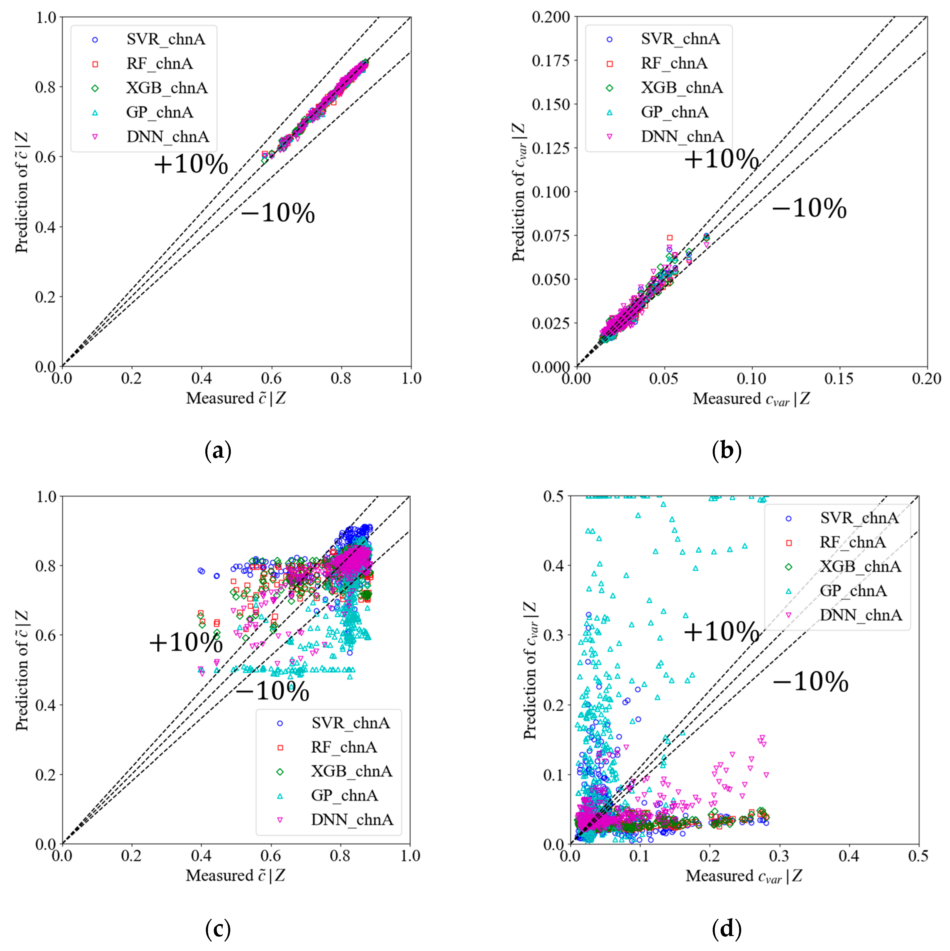
4.1. Direct Comparison of Model Predictions

As discussed in Section 2, there exists a fundamental distinction between the first four parameters and the fifth parameter. The first four parameters, Z ~ , c ~ , Z v a r , c v a r , represent the mapping of spatial locations in the flow field onto the flamelet manifold space. This implies that sampling more locations in experiments could expand the model’s applicable range for these four parameters.
However, the number of sampling positions in a single experiment is always limited. To address this issue, we propose a data fusion approach in this work. By combining training sets from different experiments to create a fusional training set, we examine whether models trained on such fusional datasets can maintain the same prediction performance comparable to those trained on individual datasets. The model will be evaluated across different test sets. This capability serves as the key criterion for assessing the effectiveness of data fusion.
In this paper, five ML models are studied. Since each model has been trained on three training sets (chnA, SM1 and data fusion), there are a total of 15 pre-trained models, as shown in Table 3:
The prediction results for the chnA’s test set and SM1’s test set are presented in Figure 3 and Figure 4, respectively. Each figure contains two columns representing the model predictions for conditional mean,   c ~ | Z , and conditional normalized variance, c v a r | Z . The three rows in each figure correspond to models trained using three different training sets. Different machine learning models are represented by scatter points with varying colors and shapes in the figures.
Firstly, the effectiveness of the hyperparameter selection and training procedure can be demonstrated by the prediction accuracy shown in Figure 3a,b and Figure 4c,d. After ruling out inadequate model training as a potential cause, the poor performance observed in Figure 3c,d and Figure 4a,b reveals that pretrained models fail to achieve effective cross-flame predictions for conditional statistics.
Further comparison of Figure 3e,f and Figure 4e,f demonstrates that models trained with data fusion can successfully predict cross-condition test cases. Notably, these fused-data models maintain prediction accuracy comparable to that shown in Figure 3a,b and Figure 4c,d, with no observable degradation in performance.
These results not only validate the efficacy of the data fusion, but also suggest that the data-driven coupling method for conditional probability distributions has considerable generalizability. This work establishes a methodological framework for data-driven PDF modeling, offering significant implications for the field.
The fundamental rationale of effective data fusion is the dimension reduction of FGM In the FGM method, flame characteristics are reduced to a low-dimensional space defined by the mixture fraction and progress variable. For turbulent flames, this corresponds to a 4D space of Z ~ c ~ Z v a r c v a r . While the flow-field characteristics of different flames influence the spatial distributions of these four statistical quantities, they do not alter the mapping relationship between flame characteristics and these parameters. Since the ML modeling in the conditional β PDF framework targets this mapping relationship, data fusion across different flames can effectively extend the model’s applicability range.
By treating the values of Z ~ , c ~ , Z v a r , c v a r as coordinates in 4D space, we can construct the 4D convex hull for a dataset. To visualize this 4D convex hull, we present its projections onto six 2D planes, as shown in Figure 5. It can be found that the datasets from two different flames exhibit both overlapping and non-overlapping domains in this 4D space. The results presented in Figure 3e,f and Figure 4e,f demonstrate that the mapping relationships within overlapping domains remain consistent across different flames. If this were not the case, a single model could not yield accurate predictions for both flames. This consistency provides the foundation for implementing data fusion. Furthermore, the ability of data fusion to extend the model’s predictive scope arises from the complementary nature of non-overlapping domains in 4D space.
For quantitative evaluation of different models, the different evaluation metrics are summarized in Table 4. The metrics include maximum error and the ratio of predictions with less than 10% error. All models were trained by a fusional training set. All metrics were calculated separately for both flame datasets. The best-performing values for each metric are highlighted in bold.
Based on a comprehensive evaluation of all metrics, the two non-parametric models, RF and GPR, demonstrated superior performance. This can be attributed to their inherent data-dependent structural characteristics. Considering that GPR requires longer training times than RF, the latter emerges as the more favorable choice.
Notably, the DNN, being the only deep learning model among the five methods, did not exhibit better performance. Given the limited dataset available for this specific problem, further improvement of the DNN’s prediction accuracy would require extensive exploration of network architectures and more advanced training techniques such as transfer learning. These approaches would increase model training complexity. In contrast, machine learning models like RF can achieve the desired predictive performance with lower costs. After comprehensive evaluation, RF emerges as the optimal solution for this specific problem.

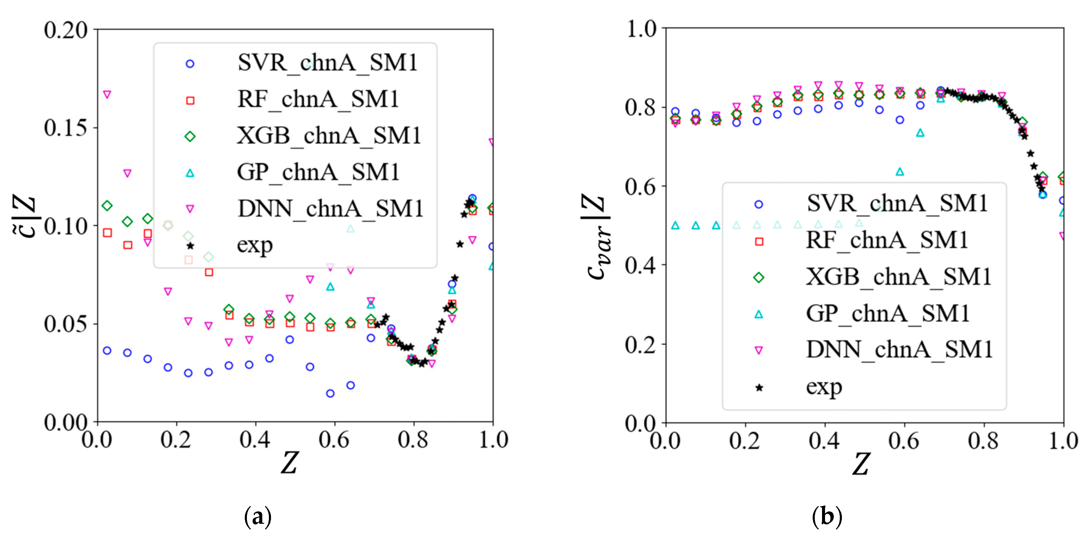
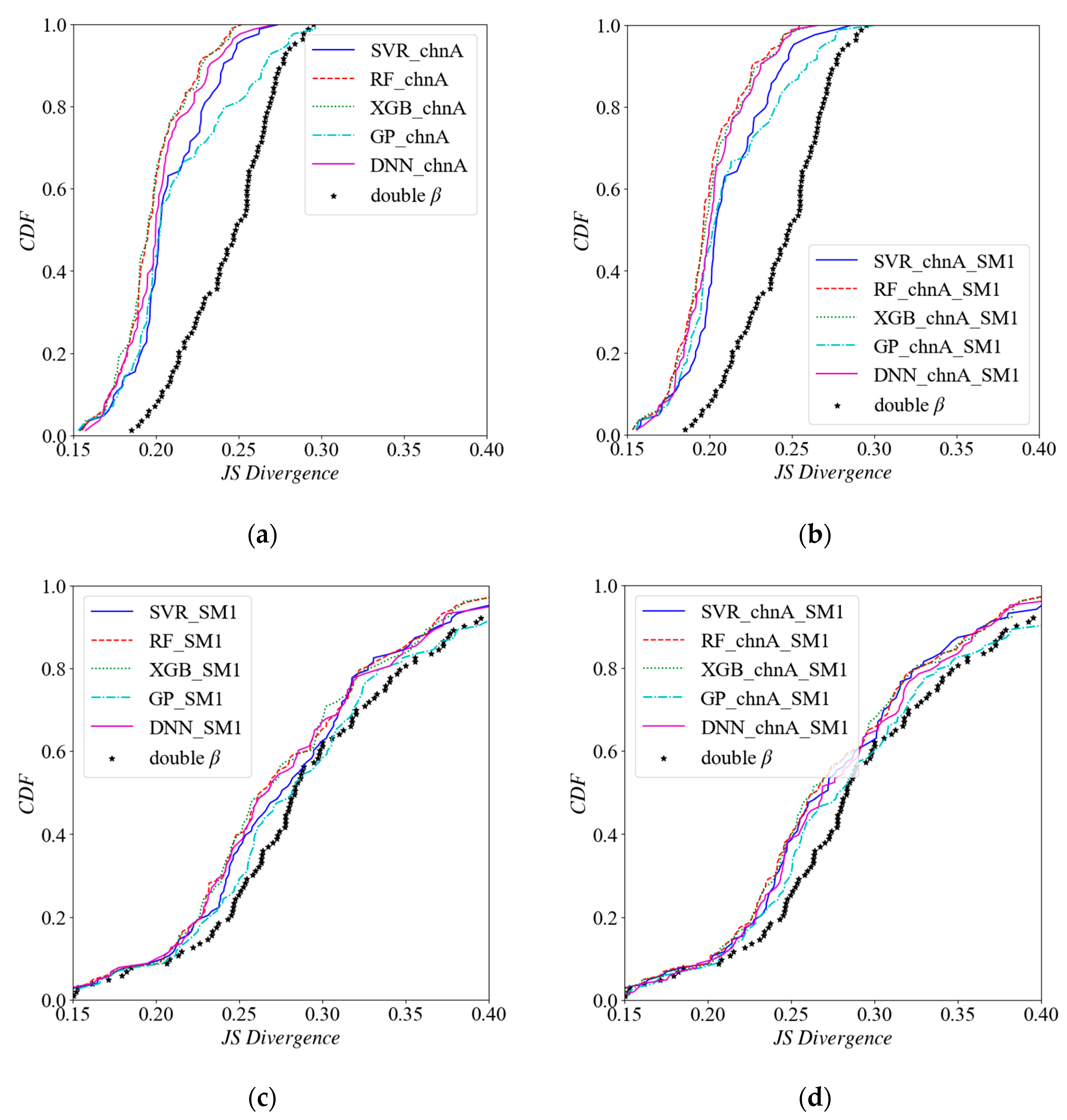
4.2. Comparison of Joint PDF

The discussion in Section 4.1 demonstrates the feasibility of data fusion, which can effectively mitigate the prediction errors caused by extrapolation of the first four parameters to some extent. The fifth parameter, denoted as condition Z , which has a defined range of [ 0 ,   1 ] , is introduced during the double integration process.
The P ( Z ) is not a constant function. In some low-probability interval, even with extensive repeated measurements at the same location, it remains challenging to obtain conditional statistics, c ~ | Z and c v a r | Z . Notably, these low-probability intervals correspond to areas with low weights in the integration process according to Equation (10). An example of a certain location in chnA is shown in Figure 6. It is impossible to obtain c ~ | Z and c v a r | Z in the interval of [0.8, 1] from the scatterplot. However, P Z in this interval is close to 0. Consequently, for extrapolation issues concerning the fifth parameter, conditional Z , predictions are generally acceptable as long as no extreme outliers occur.
In order to compare the effect of different ML models on the extrapolation of conditional Z , the predictions of c ~ | Z , and c v a r | Z , were compared for different conditions Z at different locations in the flame. And two-dimensional (2D) contours of the joint PDF at different locations in the flame are compared.
Due to space limitations, we present only two representative contour plots to discuss the impact of extrapolation of conditional Z on joint PDF. A comprehensive quantitative comparison of joint PDF predictions across all locations will be conducted using Jensen–Shannon divergence. The selected representative positions are as follows: (1) Point A: axial position z = 20   d and radial position r = 10   m m in Flame chnA; (2) Point B: axial position z = 10   m m and radial position r = 1.5   m m in Flame SM1.
Figure 7 and Figure 8 present the conditional statistics prediction results and 2D contours of joint PDF for Point A, respectively, while Figure 9 and Figure 10 show the corresponding results for Point B. In the conditional statistics prediction plots, the experimental statistical results are represented by black star symbols. All models were trained by the fusional training set.
For Point A, Figure 7 shows that the GP prediction exhibits significant instability in the extrapolation. However, the comparison of joint PDF contours in Figure 8 shows that the difference in extrapolation has a negligible impact on the joint PDF. This phenomenon occurs because the probability distribution of Z at Point A is concentrated within the interval of (0, 0.25).
The primary distinction between Point B and Point A lies in the non-negligible probability distribution of Z across the interval (0.2, 0.9) at Point B, which is shown in Figure 10. The extrapolation on Point B is due to the limited number of experimental measurements available. In this case, the instability of GP predictions in the extrapolation interval, which is shown as Figure 9 significantly impacts the resulting joint PDF in Figure 10.
It should be noted that instability in extrapolation does not necessarily lead to worse results because we lack direct validation data for these regions. However, its uncontrollable nature is undesirable in constructing data-driven models. From this perspective, random forest and XGBoost emerges as a preferable choice. Because a decision tree can be regarded as a step function in regression and random forest is inherently a superposition of step functions, which can prevent the divergence in extrapolation intervals.
The contours of joint PDF can visualize the location of differences between PDFs, but cannot be used to quantify them. In this paper, we use the Jensen–Shannon divergence (JSD) [50] to quantify the differences between the model-predicted PDFs and the experimental distributions. JSD is a symmetric version of the Kullback–Leibler divergence (KLD) [51]. The KLD and the JSD are defined in Equation (18) and Equation (19), respectively. JSD decreases as the two PDFs become more similar, reaching its minimum value of 0 when the PDFs are identical.
K P , Q = p x log 2 p x q ( x )  
J P , Q = 1 2 K P , 1 2 P + Q + K Q , 1 2 P + Q
It should be noted that the JSD is fundamentally a divergence measure rather than a true metric, as it does not satisfy the triangle inequality. In practical applications, its square root is typically employed and the logarithmic base in KLD is set to e (natural logarithm). All subsequent results presented in this paper are computed using this approach, while still being referred to as JSD for consistency.
There are 84 locations that can provide a joint PDF for validation in Flame chnA and 103 locations in Flame SM1. After computing the JSD values between the predicted PDF and experimental PDF at all locations for each model, we obtain the cumulative distribution function of JSD for different models under two flames, as shown in Figure 11. The results obtained from the double- β PDF were employed as a benchmark for comparison.
Figure 11a,c displays the results from models trained on the chnA and SM1 datasets individually, while Figure 11b, d presents those obtained using the fusional training set. No significant differences are observed between these two sets of results, demonstrating the feasibility of the data fusion strategy at the joint PDF prediction level.
Comparative analysis of the results with the double- β PDF shows that all conditional β PDFs coupled with different ML methods demonstrate closer agreement with the experimental distributions. However, the model optimization proves less effective for the Flame SM1 than Flame chnA. This limitation arises because the presumed β PDF can not model the mixture fraction distribution very well in Flame SM1, which is a representative swirling flame. When errors exist in the mixture fraction PDF, the decline in JSD will be limited regardless of how well the conditional PDF of progress variable is optimized.
A comparison of the JSD across the five ML models shows that the DNN’s performance is better than the results observed in Section 4.1. This finding indirectly validates the significance of examining model’s extrapolation behavior with respect to condition Z . Additionally, RF and XGBoost exhibit their superior performance among all models, which aligns perfectly with our previous theoretical analysis of its extrapolation characteristics.

5. Conclusions

To reconstruct the presumed PDF in the FGM method, modeling approaches that combine sparse data with prior knowledge have begun to be investigated. In this work, five different machine learning methods were coupled with conditional β distribution to obtain presumed PDF. The predictive performance of five machine learning models were systematically compared and the data fusion strategy was applied with different machine learning methods to expand the model’s applicable range.
For the direct prediction of conditional statistics, all five models’ prediction errors are acceptable. The Deep Neural Network—being the only deep learning approach among the five methods—did not exhibit better predictive performance compared to traditional machine learning methods such as Random Forest. Considering the balance between training cost and prediction accuracy. The Random Forest is the optimal choice while using the conditional β PDF model.
To address the specific challenges of reconstructing presumed PDFs, a comparative analysis of data fusion and the extrapolation characteristics of different models were conducted. The comparative study of model extrapolation behaviors shows that Random Forest has more robustness in joint PDF reconstructions, as its predictions remain constrained by the training data distribution. Furthermore, the data fusion across different flames demonstrate their significant effectiveness in expanding model applicability, with consistent improvements observed for all machine learning methods investigated in this study. The rationality of the data fusion strategy is explained from the perspective of low-dimensional space mapping. These findings carry important implications for building data-driven models in sparse-data scenarios. When more types of flame experimental data are obtained in the future, the model’s generalizability will be further improved.

Author Contributions

Conceptualization, G.Z., G.Y. and Y.W.; methodology, G.Z. and Y.W.; software, G.Z. and J.L.; validation, G.Z. and J.L.; formal analysis, G.Z.; investigation, G.Z. and Y.W.; resources, G.Z. and J.L.; data curation, G.Z.; writing—original draft, G.Z.; writing—review and editing, G.Y. and Y.W.; visualization, G.Z.; supervision, G.Y. and Y.W.; project administration, G.Y. and Y.W.; funding acquisition, Y.W. All authors have read and agreed to the published version of the manuscript.

Funding

This work is supported by the Science and Technology Plan Project of Yunnan Province, 202302AQ370003-2, National Science and Technology Major Project (2019-I-0022-0021), and the Creative Seed Fund of Shanxi Research Institute for Clean Energy, Tsinghua University.

Data Availability Statement

The data that support the findings of this study are available from the corresponding author upon reasonable request.

Conflicts of Interest

The authors declare no conflicts of interest.

References

  1. Pope, S.B. Small Scales, Many Species and the Manifold Challenges of Turbulent Combustion. Proc. Combust. Inst. 2013, 34, 1–31. [Google Scholar] [CrossRef]
  2. van Ojien, J.A.; de Goey, L.P.H. Modelling of Premixed Laminar Flames Using Flamelet-Generated Manifolds. Combust. Sci. Technol. 2000, 161, 113–137. [Google Scholar] [CrossRef]
  3. Zhang, G.; Wu, Y.; Wu, J.; Zhang, Y.; Zhang, H. State of the Art and Challenges of Flamelet Method in Gas Turbine Combustor Simulation. J. Tsinghua Univ. (Sci. Technol.) 2023, 63, 505–520. [Google Scholar]
  4. Pierce, C.D.; Moin, P. Progress-Variable Approach for Large-Eddy Simulation of Non-Premixed Turbulent Combustion. J. Fluid Mech. 2004, 504, 73–97. [Google Scholar] [CrossRef]
  5. Peters, N. Laminar Diffusion Flamelet Models in Non-Premixed Turbulent Combustion. Prog. Energy Combust. Sci. 1984, 10, 319–339. [Google Scholar] [CrossRef]
  6. Cook, A.W.; Riley, J.J. A Subgrid Model for Equilibrium Chemistry in Turbulent Flows. Phys. Fluids 1994, 6, 2868–2870. [Google Scholar] [CrossRef]
  7. Ramaekers, W.J.S.; Albrecht, B.A.; van Oijen, J.A.; de Goey, L.P.H. The Application of Flamelet Generated Manifolds in Partailly-Premixed Flames. In Proceedings of the Fluent Benelux User Group Meeting, Wavre, Belgium, 6–7 October 2005. [Google Scholar]
  8. Vreman, A.W.; Albrecht, B.A.; van Oijen, J.A.; de Goey, L.P.H. Premixed and Nonpremixed Generated Manifolds in Large-Eddy Simulation of Sandia Flame D and F. Combust. Flame 2008, 153, 394–416. [Google Scholar] [CrossRef]
  9. Grout, R.W.; Swaminathan, N.; Cant, R.S. Effects of Compositional Fluctuations on Premixed Flames. Combust. Theory Model. 2009, 13, 823–852. [Google Scholar] [CrossRef]
  10. Zhang, W.; Karaca, S.; Wang, J.; Huang, Z.; van Oijen, J. Large Eddy Simulation of the Cambridge/Sandia Stratified Flame with Flamelet-Generated Manifolds: Effects of Non-Unity Lewis Numbers and Stretch. Combust. Flame 2021, 227, 106–119. [Google Scholar] [CrossRef]
  11. Popov, P.P. Alternatives to the Beta Distribution in Assumed PDF Methods for Turbulent Reactive Flow. Flow Turbul. Combust. 2022, 108, 433–459. [Google Scholar] [CrossRef]
  12. Salehi, M.M.; Bushe, W.K.; Shahbazian, N.; Groth, C.P.T. Modified Laminar Flamelet Presumed Probability Density Function for LES of Premixed Turbulent Combustion. Proc. Combust. Inst. 2013, 34, 1203–1211. [Google Scholar] [CrossRef]
  13. Ghadimi, M.; Atayizadeh, H.; Salehi, M.M. Presumed Joint-PDF Modelling for Turbulent Stratified Flames. Flow Turbul. Combust. 2021, 107, 405–439. [Google Scholar] [CrossRef]
  14. Darbyshire, O.R.; Swaminathan, N. A Presumed Joint Pdf Model for Turbulent Combustion with Varying Equivalence Ratio. Combust. Sci. Technol. 2012, 184, 2036–2067. [Google Scholar] [CrossRef]
  15. Zhang, H.; Yu, Z.; Ye, T.; Cheng, M.; Zhao, M. Large Eddy Simulation of Turbulent Stratified Combustion Using Dynamic Thickened Flame Coupled Tabulated Detailed Chemistry. Appl. Math. Model. 2018, 62, 476–498. [Google Scholar] [CrossRef]
  16. Ruan, S.; Swaminathan, N.; Darbyshire, O. Modelling of Turbulent Lifted Jet Flames Using Flamelets: A Priori Assessment and a Posteriori Validation. Combust. Theory Model. 2014, 18, 295–329. [Google Scholar] [CrossRef]
  17. Chen, Z.X.; Doan, N.A.K.; Ruan, S.; Langella, I.; Swaminathan, N. A Priori Investigation of Subgrid Correlation of Mixture Fraction and Progress Variable in Partially Premixed Flames. Combust. Theory Model. 2018, 22, 862–882. [Google Scholar] [CrossRef]
  18. Jaganath, V.; Stoellinger, M. Transported and Presumed Probability Density Function Modeling of the Sandia Flames with Flamelet Generated Manifold Chemistry. Phys. Fluids 2021, 33, 045123. [Google Scholar] [CrossRef]
  19. Jordan, M.I.; Mitchell, T.M. Machine Learning: Trends, Perspectives, and Prospects. Science 80 2015, 349, 255–260. [Google Scholar] [CrossRef]
  20. Agrawal, A.; Choudhary, A. Perspective: Materials Informatics and Big Data: Realization of the “Fourth Paradigm” of Science in Materials Science. APL Mater. 2016, 4, 053208. [Google Scholar] [CrossRef]
  21. Afanaseva, O.V.; Tulyakov, T.F. Comparative Analysis of Image Segmentation Methods in Power Line Monitoring Systems. Int. J. Eng. Trans. A Basics 2026, 39, 1–11. [Google Scholar] [CrossRef]
  22. Brunton, S.L.; Noack, B.R.; Koumoutsakos, P. Machine Learning for Fluid Mechanics. Annu. Rev. Fluid Mech. 2020, 52, 477–508. [Google Scholar] [CrossRef]
  23. Raissi, M.; Yazdani, A.; Karniadakis, G.E. Hidden Fluid Mechanics: Learning Velocity and Pressure Fields from Flow Visualizations. Science 80 2020, 367, 1026–1030. [Google Scholar] [CrossRef]
  24. An, J.; Chen, Y.; Su, X.; Zhou, H.; Ren, Z. Applications and Prospects of Machine Learning in Turbulent Combustion and Engines. J. Tsinghua Univ. 2023, 63, 462–472. [Google Scholar]
  25. Liu, J.; Liu, G.; Wu, J.; Zhang, G.; Wu, Y. Prediction of Flame Type and Liftoff Height of Fuel Jets in Turbulent Hot Coflow Using Machine Learning Methods. Combust. Sci. Technol. 2025, 197, 1760–1782. [Google Scholar] [CrossRef]
  26. Zeng, J.; Cao, L.; Xu, M.; Zhu, T.; Zhang, J.Z.H. Complex Reaction Processes in Combustion Unraveled by Neural Network-Based Molecular Dynamics Simulation. Nat. Commun. 2020, 11, 5713. [Google Scholar] [CrossRef]
  27. Ji, W.; Deng, S. Autonomous Discovery of Unknown Reaction Pathways from Data by Chemical Reaction Neural Network. J. Phys. Chem. A 2021, 125, 1082–1092. [Google Scholar] [CrossRef]
  28. Mirgolbabaei, H.; Echekki, T. A Novel Principal Component Analysis-Based Acceleration Scheme for LES-ODT: An a Priori Study. Combust. Flame 2013, 160, 898–908. [Google Scholar] [CrossRef]
  29. Malik, M.R.; Coussement, A.; Echekki, T.; Parente, A. Principal Component Analysis Based Combustion Model in the Context of a Lifted Methane/Air Flame: Sensitivity to the Manifold Parameters and Subgrid Closure. Combust. Flame 2022, 244, 112134. [Google Scholar] [CrossRef]
  30. Wu, J.; Zhang, S.; Wu, Y.; Zhang, G.; Li, X.; Zhang, H. FlamePINN-1D: Physics-Informed Neural Networks to Solve Forward and Inverse Problems of 1D Laminar Flames. Combust. Flame 2025, 273, 113964. [Google Scholar] [CrossRef]
  31. Song, M.; Tang, X.; Xing, J.; Liu, K.; Luo, K.; Fan, J. Physics-Informed Neural Networks Coupled with Flamelet/Progress Variable Model for Solving Combustion Physics Considering Detailed Reaction Mechanism. Phys. Fluids 2024, 36, 103616. [Google Scholar] [CrossRef]
  32. Chen, Z.X.; Iavarone, S.; Ghiasi, G.; Kannan, V.; D’Alessio, G.; Parente, A.; Swaminathan, N. Application of Machine Learning for Filtered Density Function Closure in MILD Combustion. Combust. Flame 2021, 225, 160–179. [Google Scholar] [CrossRef]
  33. Henry de Frahan, M.T.; Yellapantula, S.; King, R.; Day, M.S.; Grout, R.W. Deep Learning for Presumed Probability Density Function Models. Combust. Flame 2019, 208, 436–450. [Google Scholar] [CrossRef]
  34. Gitushi, K.M.; Ranade, R.; Echekki, T. Investigation of Deep Learning Methods for Efficient High-Fidelity Simulations in Turbulent Combustion. Combust. Flame 2022, 236, 111814. [Google Scholar] [CrossRef]
  35. Zhang, G.; Li, X.; Wu, Y.; Zhang, R.; Guo, H.; Yue, G. A Data Driven Conditional Presumed PDF Generation Method for FGM with Random Forest Model. Combust. Sci. Technol. 2025, 00, 1–27. [Google Scholar] [CrossRef]
  36. Minamoto, Y.; Swaminathan, N.; Cant, R.S.; Leung, T. Reaction Zones and Their Structure in MILD Combustion. Combust. Sci. Technol. 2014, 186, 1075–1096. [Google Scholar] [CrossRef]
  37. Breiman, L. Random Forests. Mach. Learn. 2001, 45, 5–32. [Google Scholar] [CrossRef]
  38. Quinlan, J.R. Induction of Decision Trees. Mach. Learn. 1986, 1, 81–106. [Google Scholar] [CrossRef]
  39. Chen, T.; Guestrin, C. XGBoost: A Scalable Tree Boosting System. In Proceedings of the 22nd ACM SIGKDD International Conference on Knowledge Discovery and Data Mining, San Francisco, CA, USA, 13 August 2016; pp. 785–794. [Google Scholar]
  40. Cortes, C.; Vapnik, V. Support-Vector Networks. Mach. Learn. 1995, 20, 273–297. [Google Scholar] [CrossRef]
  41. Vapnik, V.; Golowich, S.E.; Smola, A. Support Vector Method for Function Approximation, Regression Estimation, and Signal Processing. In Proceedings of the 10th International Conference on Neural Information Processing Systems, Cambridge, MA, USA, 3 December 1996; pp. 281–287. [Google Scholar]
  42. O’Hagan, A. Curve Fitting and Optimal Design for Prediction. J. R. Stat. Soc. B 1978, 40, 1–24. [Google Scholar] [CrossRef]
  43. Rasmussen, C.E.; Williams, C.K.I. Gaussian Processes for Machine Learning; MIT Press: Cambridge, MA, USA, 2006; Volume 7, ISBN 026218253X. [Google Scholar]
  44. Jain, A.K.; Mao, J.; Mohiuddin, K.M. Artificial Neural Networks: A Tutorial. Computer 1996, 29, 31–44. [Google Scholar] [CrossRef]
  45. Barlow, R.S.; Fiechtner, G.J.; Carter, C.D.; Chen, J.Y. Experiments on the Scalar Structure of Turbulent CO/H2/N2 Jet Flames. Combust. Flame 2000, 120, 549–569. [Google Scholar] [CrossRef]
  46. Al-Abdeli, Y.M.; Masri, A.R. Stability Characteristics and Flowfields of Turbulent Non-Premixed Swirling Flames. Combust. Theory Model. 2003, 7, 731–766. [Google Scholar] [CrossRef]
  47. Masri, A.R.; Kalt, P.A.M.; Barlow, R.S. The Compositional Structure of Swirl-Stabilised Turbulent Nonpremixed Flames. Combust. Flame 2004, 137, 1–37. [Google Scholar] [CrossRef]
  48. Masri, A.R.; Bilger, R.W.; Dibble, R.W. Turbulent Nonpremixed Flames of Methane near Extinction: Probability Density Functions. Combust. Flame 1988, 73, 261–285. [Google Scholar] [CrossRef]
  49. Ma, L. Computational Modeling of Turbulent Spary Combustion. Doctoral Thesis, Delft University of Technology, Delft, The Netherlands, 2016. [Google Scholar]
  50. Lin, J. Divergence Measures Based on the Shannon Entropy. IEEE Trans. Inf. Theory 1991, 37, 145–151. [Google Scholar] [CrossRef]
  51. Kullback, S.; Leibler, R.A. On Information and Sufficiency. Ann. Math. Stat. 1951, 22, 79–86. [Google Scholar] [CrossRef]
Figure 1. Schematic diagram of five different models.
Energies 18 03546 g001
Figure 2. Representative example of invalid measurement locations.
Energies 18 03546 g002
Figure 3. The prediction results for chnA’s test set: (a) conditional mean of model trained by chnA’s training set; (b) conditional normalized variance of model trained by chnA’s training set; (c) conditional mean of model trained by SM1’s training set; (d) conditional normalized variance of model trained by SM1’s training set; (e) conditional mean of model trained by fusional training set; (f) conditional normalized variance of model trained by fusional training set.
Energies 18 03546 g003aEnergies 18 03546 g003b
Figure 4. The prediction results for SM1’s test set: (a) conditional mean of model trained by chnA’s training set; (b) conditional normalized variance of model trained by chnA’s training set; (c) conditional mean of model trained by SM1’s training set; (d) conditional normalized variance of model trained by SM1’s training set; (e) conditional mean of model trained by fusional training set; (f) conditional normalized variance of model trained by fusional training set.
Energies 18 03546 g004aEnergies 18 03546 g004b
Figure 5. The projections of 4D convex hull on different 2D planes: (a) Z ~ c ~ ; plane; (b) Z ~ Z v a r plane; (c) Z ~ c v a r plane; (d) c ~ Z v a r ; (e) c ~ c v a r plane; (f) Z v a r c v a r plane.
Energies 18 03546 g005
Figure 6. The probability distribution of a certain location in chnA: (a) scatterplot of Z and c ; (b) probability distribution function.
Energies 18 03546 g006
Figure 7. The predictions of different models at Point A: (a) c ~ | Z ; (b) c v a r | Z .
Energies 18 03546 g007
Figure 8. The contours of joint PDF with different models at Point A.
Energies 18 03546 g008
Figure 9. The predictions of different models at Point B: (a) c ~ | Z ; (b) c v a r | Z .
Energies 18 03546 g009
Figure 10. The contours of joint PDF with different models at Point B.
Energies 18 03546 g010
Figure 11. The cumulative distribution function of JSD for different models. (a) the results of Flame chnA with models trained by chnA’s training set; (b) the results of Flame chnA with models trained by fusional training set; (c) the results of Flame SM1 with models trained by SM1’s training set; (d) the results of Flame SM1 with models trained by fusional training set.
Energies 18 03546 g011
Table 1. Information of flame chnA.
Nozzle ID (mm)Nozzle OD (mm) U j (m/s) R e j e t
4.586.3476.0 ± 1.5~16,700
Table 2. Information of flame SM1.
U j (m/s) U s (m/s) U e (m/s) W s (m/s) R e j e t R e s
32.738.22019.1720075,900
Table 3. Information on different models.
Models’ NameML MethodsTraining Set
SVR_chnASupport Vector RegressionchnA’s training set
RF_chnARandom ForestchnA’s training set
XGB_chnAXGBoostchnA’s training set
GP_chnAGaussian Process RegressionchnA’s training set
DNN_chnADeep neural networkchnA’s training set
SVR_SM1Support Vector RegressionSM1’s training set
RF_SM1Random ForestSM1’s training set
XGB_SM1XGBoostSM1’s training set
GP_SM1Gaussian Process RegressionSM1’s training set
DNN_SM1Deep neural networkSM1’s training set
SVR_chnA_SM1Support Vector Regressionfusional training set
RF_chnA_SM1Random Forestfusional training set
XGB_chnA_SM1XGBoostfusional training set
GP_chnA_SM1Gaussian Process Regressionfusional training set
DNN_chnA_SM1Deep neural networkfusional training set
Table 4. Evaluation metrics of different models.
Table SetsMetrics TypeSVRRFXGBGPRDNN
chnAmax error for c ~ | Z 3.4%1.9%3.2%2.4%3.1%
ratio of error < 10% for c ~ | Z 100%100%100%100%100%
max error of c v a r | Z 29.5%19.2%27.5%15.8%32.2%
ratio of error < 10% for c v a r | Z 91.9%98.0%97.7%97.2%77.5%
SM1max error of c ~ | Z 2.9%8.2%11.4%2.4%8.1%
ratio of error < 10% for c ~ | Z 100%100%99.5%100%100%
max error of c v a r | Z 50.4%22.8%39.1%22.5%70.1%
ratio of error < 10% for c v a r | Z 84.4%95.2%94.1%90.5%65.0%
Disclaimer/Publisher’s Note: The statements, opinions and data contained in all publications are solely those of the individual author(s) and contributor(s) and not of MDPI and/or the editor(s). MDPI and/or the editor(s) disclaim responsibility for any injury to people or property resulting from any ideas, methods, instructions or products referred to in the content.

