Abstract
This paper presents a proposed error model for the signal errors resulting from delays in the measurement chain. The analysis focuses on the uncertainty budget of the input quantities in the digital signal-processing algorithm, examining the influence of delays in the analog-to-digital processing stage on the uncertainty of these quantities. A classification of delays, based on their properties and the nature of the error signal they generate, is proposed. In addition to the mathematical model and its verification through the Monte Carlo method, the paper discusses potential applications of the proposed analysis method for selected implementations of measurement chains. This method can be utilized for power and energy measurement, power grid fault detection, and the identification of short circuits, among other applications.
1. Introduction
Digital data-processing (D/D) algorithms are used in virtually every measurement chain. They are applied in both static and dynamic reproduction of the measured quantity [1,2,3], spectral analysis of the signal [4,5,6,7], power and energy measurements [8,9], medicine [10,11], diagnostics [12,13], and power grid fault detection [14,15]. The delay phenomena discussed also apply in situations in which the delay occurs due to the time needed for communication between the systems used, as described, among others, in [16]. A common feature of all the above-mentioned applications is a fragment of analog-to-digital (A/D) processing, the task of which is to convert subsequent realizations of the measured quantity , represented by voltage , into subsequent discrete samples .
While the literature often discusses issues related to the properties of the A/D converter in the uncertainty budget of quantity [17,18,19,20], these considerations rarely address the problem of delays occurring in the A/D conversion process. However, this issue is very important in the context of algorithms that process sequences N of successive samples of , such as Wavelet Transform (WT) or Discrete Fourier Transform (DFT) algorithms.
So far, in the literature [21,22,23,24], there have been proposals for a general error model related to such delays. However, these were Polish-language publications of local scope and were not presented in the international literature. The model proposed in the indicated works presents a general outline of how to define the discussed error signal, but does not indicate how to determine its parameters and does not propose a division of the components of this signal due to the nature of their implementation. The indicated division is important due to the analysis of how the discussed error signal is processed by the D/D algorithm used in the measurement chain. Delay problems were also addressed, among others, in [25,26,27,28,29]; however, the considerations and models proposed therein are not directly applicable in the case of using digital signal-processing (DSP) algorithms, as mentioned in previous studies. The methods indicated in the above-mentioned works focus on specific applications, which makes it difficult to use them in general cases by using a different solution of the measurement chain. A similar situation applies to the JCGM Guide [30], as no procedure is indicated therein for estimating the measurement uncertainty in the discussed case.
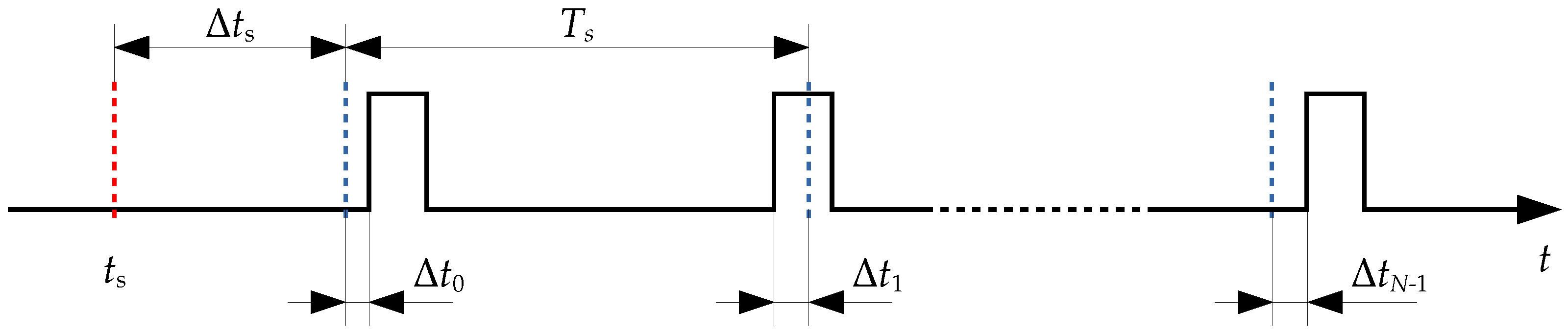
In analyzing the process of acquiring successive samples of quantity , two main problems can be observed: the process of initiating the measurement and the process of collecting successive samples of quantity . Measurement initiation is usually triggered by the detection of an appropriate condition (e.g., detection of a phenomenon or a signal crossing a set threshold). It can be noted here that the value of the first sample is acquired after a certain time . The introduced delay is related, among others, to the phenomenon detection time [26,28] (i.e., the time for performing the measurement examining the phenomenon and for executing the detection algorithm), as well as to the possible concurrent execution of other tasks [31,32] (including task preemption). When the measurement has been initiated and N subsequent values of are being collected, these values should be acquired at constant time intervals , where is the sampling frequency, constant for all samples. In reality, however, this frequency may fluctuate, causing each sample to be shifted by a time , which may differ for each sample. These phenomena are shown in Figure 1.
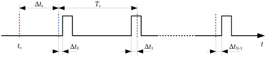
Figure 1.
The phenomenon of delays during analog-to-digital conversion. The red line indicates the start of the measurement in the ideal situation, the blue lines indicate the sampling time for a constant sampling period , and the rising edges indicate the actual sampling time.
Taking into account the current state of knowledge and the popularity of digital data-processing algorithms, this paper proposes an error model for the phenomena discussed in the introduction and presented in Figure 1. The proposed model enables analytical determination of the variance of error signals related to delays, eliminating the need for Monte Carlo simulation [3,33,34] and thereby saving the time-consuming effort involved in conducting experiments. In addition to theoretical considerations, the paper includes a description and the results of several experiments verifying the effectiveness of the proposed method, as well as examples of its application in cases involving solutions such as “system-on-chip” [35] and Wavelet Transform algorithms [5].
The paper is divided into five parts: Section 1 contains an overview of the current state of knowledge and the most important assumptions. Section 2 describes the model of delay-related error signals, with derivations for selected dependencies provided in Appendix A. Section 3 presents a description and the results of experiments verifying the effectiveness of the proposed method, while Section 4 discusses its possible applications. Finally, Section 5 provides a summary and the most important conclusions regarding the proposed method.
2. Time-Related Error Model
In analyzing the case presented in Figure 1, it can be observed that delays in processing successive samples of the signal result from two main phenomena:
- , the delay in starting the measurement relative to the time , at which the measurement should begin;
- , the difference in the processing time of the i-th signal sample relative to the time expected based on the sampling period .
In the first case, the delay may result, for example, from the time required to execute the algorithm responsible for initiating the measurement under specific conditions or from waiting for available resources in the case of multi-task solutions [31,32]. In the second case, the time difference may result from fluctuations in the frequency of the clock running the counter [36], which, in turn, triggers successive measurements in the A/D converter [37].
Assuming that the signal is a discrete representation of , the ideal waveform of can be described by the following equation [38]:
where is the ideal starting time of the measurement. According to the model in Figure 1, the observed signal , affected by the error signal resulting from the delays discussed above, can be expressed as follows:
Hence, the error signal can be described by the following equation [30]:
From Figure 1, it can be seen that the delay is constant for all samples of the signal and is greater than zero. In contrast, the time difference may vary across samples and can take both negative and positive values.
By representing the signal as a sum of its harmonics [39], Equations (1) and (2) can be rewritten as follows:
Thus, the error signal corresponding to the k-th harmonic of the signal with pulsation can be written as follows:
From Equation (7), it can be seen that the characteristics of the error signal due to delays are closely correlated with the number and properties of the harmonics present in the signal . Additionally, it can be noted that, if contains a constant component, the delay-related phenomena discussed here do not introduce any error in that component.
2.1. Error Signal Related to Measurement Initiation Delay
When considering the nature of the parameter , which assumes the same value for all samples of the signal in a single measurement, it can be observed that the error signal will have a deterministic component [40,41,42], with a pulsation equal to that of the original harmonic of the signal , and an expected value of zero [39]. This is an important feature because, from the perspective of processing this component using the D/D algorithm, the processing may depend on the value of the pulsation of this harmonic [43].
The zero expected value of this component results from the fact that the “sinus” function is characterized by a zero expected value, regardless of the value of the phase parameter. Assuming the measurement process is repeated many times, the average value of the implementation of the discussed component of the error signal will be zero. Because, for a single measurement window, successive values of the discussed component correspond to successive values of the “sinus” function with pulsation , the distribution of these values forms a “U”-shaped pattern [44].
Because, in reality, the initiation delay of the measurement process is always greater than zero, this component will always be characterized by a non-zero variance for each measurement implementation. The value of this variance will be proportional to the delay implementation value . For each measurement implementation, the error signal associated with the discussed component will exhibit different variance values. By repeating the measurement multiple times, this value may change across subsequent measurement implementations; therefore, in the subsequent sections of this paper, the expected value of the variance associated with the analyzed component of the error signal will be considered [30].
2.2. Error Signal Related to Sampling Period Fluctuation
The second component of the error signal will be a random component [45] with a zero expected value and energy distributed across all pulsation values [39]. For the discussed component, it is proposed to adopt a model in which this component is a non-deterministic signal with a constant power spectral density [46]. The distribution of the realization values of this component will depend on the distribution of the parameter .
Because, for each realization of the A/D converter system, the expected value of the parameter should remain invariant, and the realization values depend on the fluctuations of this parameter, it can be assumed that the expected value of is zero. In practice, this means that the phenomenon in question is not associated with the possibility of a deterministic error signal, as discussed for the parameter . However, it should be noted that, if the expected value of were non-zero, the deterministic component would be strongly correlated with the component resulting from the parameter [39,47,48].
2.3. Delay-Related Error Signal Variance
By analyzing the case in which the measurement process is repeated many times for different realizations of and , it can be observed that, regardless of the nature of the error signals introduced by the phenomena related to them, the resultant error signal can be described in probabilistic terms [30,38,41,45,49]. It can therefore be assumed that , , and , where the symbol U denotes the uniform distribution [45]. The values of the realizations of these parameters are thus irrelevant for determining the variance of the error signal .
For the adopted assumptions, it can also be noted that, regardless of the nature of the realizations of the parameters and for a single measurement window, on a global scale, these variables can be treated as two uncorrelated random variables [45]. Based on the nature of the components of the error signal , it is therefore proposed to determine the variance of these components analytically, separately for each component. Additionally, due to the completely different nature of the realizations of these components within a single measurement window of the D/D algorithm, it is proposed to disregard any correlation between these components in the considerations. Detailed derivations are not presented in the rest of this chapter; they can be found in Appendix A.
Given the adopted assumptions, a single harmonic of the error signal , the pulsation of which is , can be described by the following equation:
where is the difference between the ideal and actual times at which the realization value of the quantity is taken.
For the assumption that the signal components associated with the parameters and are not correlated with each other, the variance of a single component of the signal in question can be determined, regardless of its nature, according to the following equation [39]:
where “∗” denotes the component of the error signal where is related to the delay in initiating the measurement process and is related to the fluctuation of the sampling period. It can be observed that, for the assumption where , regardless of the parameters of the variable , the expected value of the part related to the “cosine” function is zero, while the root mean square value of this function is [39]. For these properties, Equation (9) is transformed into the following form:
Hence, the final value of the variance for the discussed component directly depends on the signal parameters and the distribution parameters of the realization values for the analyzed delay .
In the case where , one can observe the property where . Hence, the expected value of is
while the variance of the error signal related to for the indicated parameters is described by the following equation:
The next case considered in this paper is the scenario where , where the symbol N denotes the normal distribution [45]. The expected value of is then
Therefore, the variance of the error signal related to is
For the case where , where G denotes the “Gamma” [45] distribution, the expected value of is
Therefore, for the discussed case, the variance of the error signal related to is described by the following equation:
Finally, the variance value, denoted as , for the error signal , can be estimated using the following equation:
where the variance values for each component are determined by the distribution of realizations of the parameters and , and are calculated according to Equation (10).
As per the previous discussion regarding the nature of the parameter , the literature commonly suggests the use of the “Gamma” distribution for modeling the realization values of this parameter [26,29,32,45]. For the component associated with the parameter , it is generally assumed that the number of factors influencing its realization is large enough, which justifies the use of the normal distribution [30,36]. Detailed derivations of the dependencies from Equations (11)–(16) can be found in Appendix A.
2.4. The Case of a Non-Zero Expected Value of Sampling Period Fluctuation
When the expected value of the parameter is non-zero, it is recommended to modify the method as follows:
In these assumptions, it is considered that the expected value of contributes as an additional component to the average delay value . This modification enables the proposed method to be applied directly, eliminating the need to account for the correlation between the deterministic components of the error signal .
3. Verification of the Proposed Method
The effectiveness of the proposed method was verified through simulation. For this purpose, a series of experiments was conducted using the Monte Carlo method. Each iteration of the experiment involved generating a vector of samples of size for the ideal case, according to Equation (1), and for the case where there is an error related to delays, according to Equation (2). The time value for each iteration of the experiment was randomly selected such that .
In the experiments, the measurement chain processed the signal given by Equation (4), where , , while the phase value was randomly selected for each iteration of the experiment. It was assumed that the sampling period in the ideal case was , so the sampling rate was Hz. The experiments were performed for different parameters and distributions of the realizations of the quantities and . For each set of parameters, iterations were performed, as described in the previous paragraph.
For the obtained values of the signal realization , the subsequent realizations of the error signal were determined according to Equation (3). For all obtained samples of the error signal , their variance was calculated using the following equation [30]:
Next, the variance of was estimated according to Equation (17). Then, the relative error in estimating this value was determined [30]:
According to the description presented above, the course of a single iteration of the experiment was as follows:
- Randomize the initial phase of the signal , where ;
- Generate a vector N of successive samples of quantity based on Equation (1);
- Randomize the value of the quantity according to the given parameters of the distribution of this quantity;
- Randomize a vector of N successive values of the quantity according to the given parameters of the distribution of this quantity;
- Generate a vector of N consecutive samples of the signal based on Equation (2);
- Calculate the realization values of the error signal according to Equation (3);
- Calculate the variance value of the error signal based on Equation (20);
- Estimate the variance value of the error signal based on Equation (17);
- Calculate the relative error of the estimated variance value based on Equation (21).
3.1. Case of Delay in Initiation of the Measurement Process
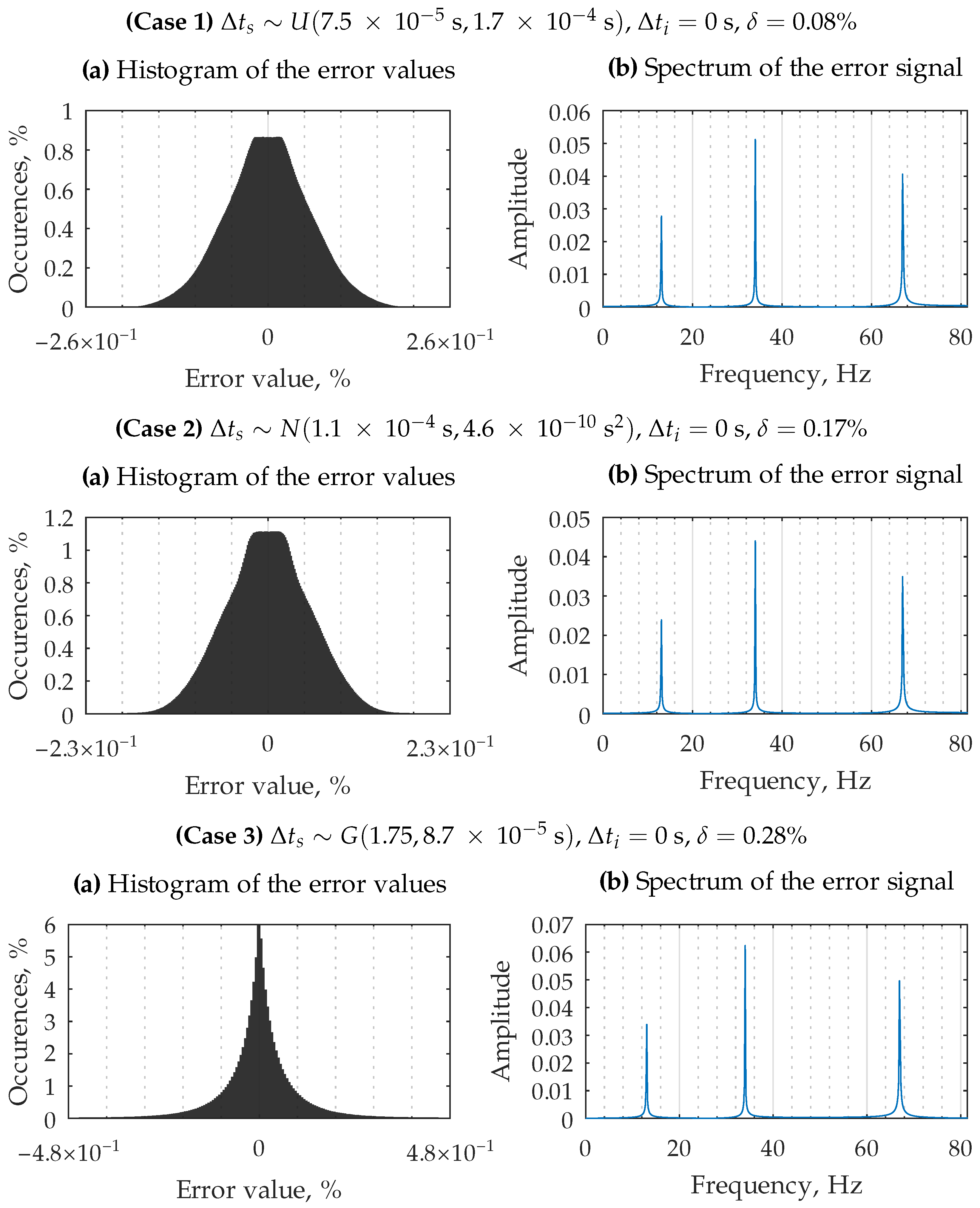
In the experiment, it was assumed that parameter , meaning there was no phenomenon of sampling period fluctuation. The parameters of the quantity were dependent on the variant of the experiment. The histograms of all realizations of the error signal related to delays are shown in Figure 2a, while the spectrum of an example vector consisting of N realizations of this signal is shown in Figure 2b. This experiment can be recreated for any parameters by running the test_var_1_*.m scripts from the repository [50]. For the discussed experiment, the parameters of the distribution of realization values of the quantity were chosen so that the inequality was satisfied.
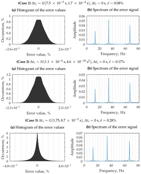
Figure 2.
Experimental results in the case of a delay in the initiation of the measurement process.
Based on the experimental results, it can be seen that the variance of the analyzed error signal was estimated correctly. It is important to note that this value applies to cases where the measurement process is repeated multiple times. For a single iteration of the experiment, the actual variance of the error signal may differ, because it is influenced directly by the nature of the signal. The signal discussed for a single measurement realization is deterministic, and its variance depends directly on the value of the realization of the parameter . This phenomenon and the nature of the signal can be observed by analyzing its spectrum, as presented in Figure 2b.
3.2. The Case with Sampling Period Fluctuation
In this variant, it was assumed that there was no delay in the initiation of the measurement process, so , while the parameters of the quantity depended on the variant of the experiment. The histograms of all realizations of the error signal associated with delays are shown in Figure 3a, while the spectrum of an example vector consisting of N realizations of this signal is shown in Figure 3b. This experiment can be reproduced with any parameters by running the test_var_2_*.m scripts from the repository [50]. For the discussed experiment, the parameters of the distribution of realization values of the quantity were chosen so that the equality was satisfied.
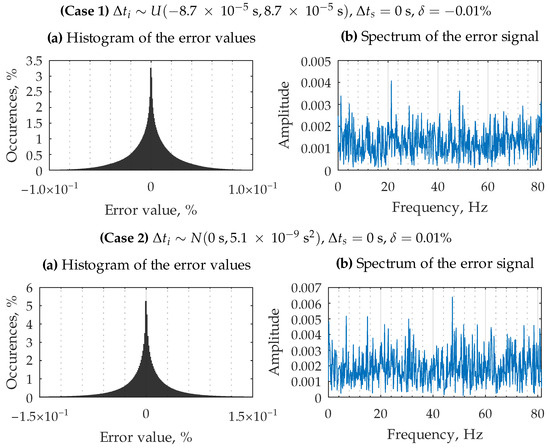
Figure 3.
Experimental results in the case of sampling period fluctuations.
The analysis of the experiment results allowed us to conclude that the parameters of the error signal related to the phenomenon of sampling period fluctuations were estimated correctly. The experiments also confirmed the properties discussed in the previous chapter and the random nature of the analyzed error signal, which can be seen by analyzing the spectrum of this signal presented in Figure 3b. In this case, for a sufficiently large number of N samples of the processed vector of quantities [30], the estimated value of the variance is correct for any realization of the measurement process.
3.3. The Case with Multiple Delay Sources
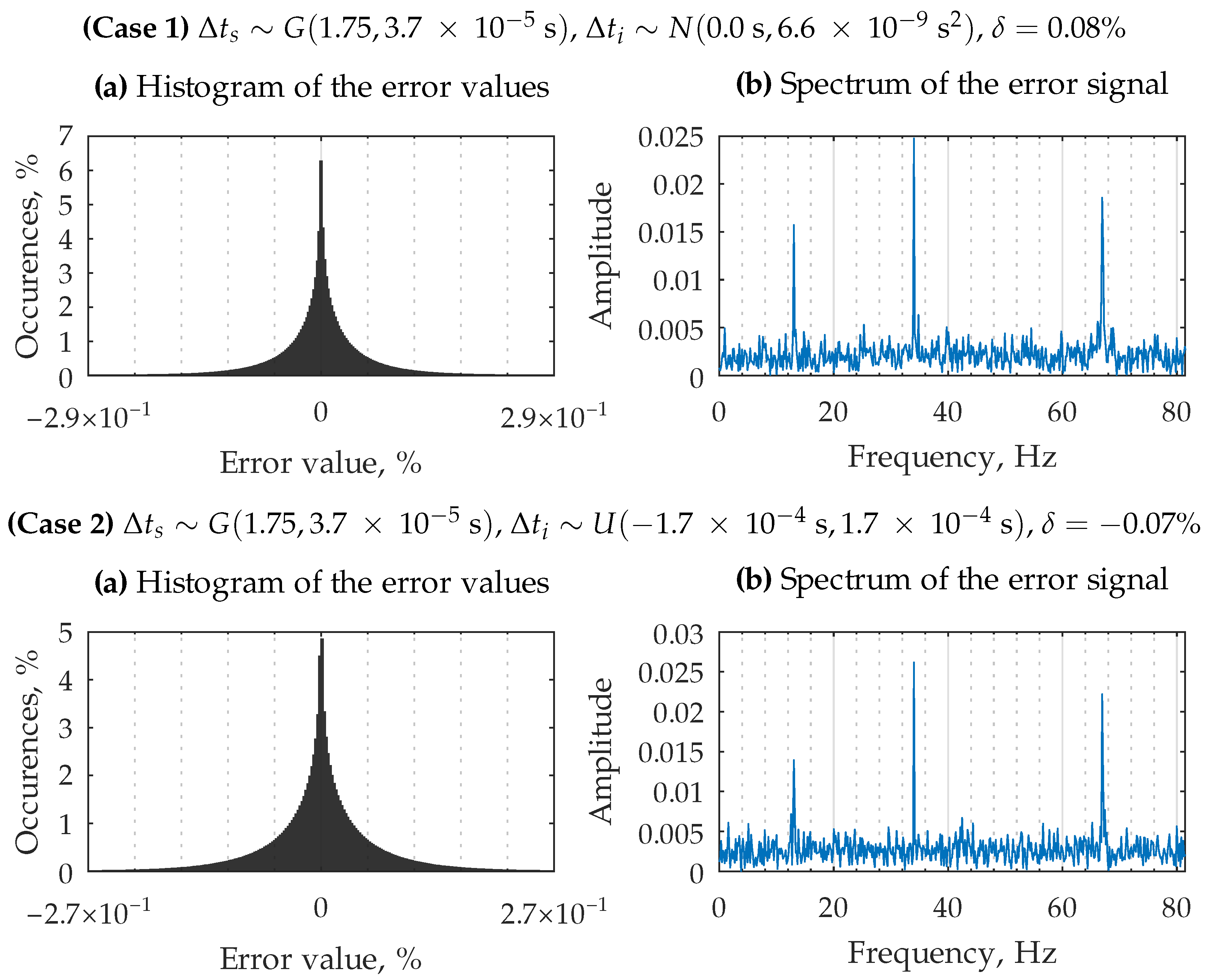
In the discussed variant, both a delay in the initiation of the measurement process and fluctuations in the sampling period were assumed. The parameters of the quantities and depended on the variant of the experiment. The histograms of all realizations of the error signal related to delays are shown in Figure 4a, while the spectrum of an example vector consisting of N realizations of this signal is shown in Figure 4b. This experiment can be reproduced with any parameters by running the test_var_3_*.m scripts from the repository [50]. For the discussed experiment, the parameters of the distribution of realization values of the quantity and were chosen to satisfy and .
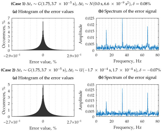
Figure 4.
Experimental results in the case of delayed measurement process initiation and sampling period fluctuations.
For the conducted experiments, the estimated variance of the error signal related to delays coincided with the reference value. This confirms that the assumption made in the previous section regarding the negligible correlation between components of the analyzed error signal is justified. By analyzing the histograms presented in Figure 4b, it can be seen that the discussed error signal contains both deterministic components, whose pulsations correspond to the harmonics of the signal , and a random component, the energy of which is uniformly distributed across the entire spectrum of the error signal.
3.4. Experiments Conclusions
The results of the conducted experiments confirm the effectiveness of the proposed method and the adopted assumptions. Although the variance of each component of the error signal resulting from delays is estimated using Equation (9) regardless of the nature of the components, it is necessary to analyze each component separately. This necessity results from the differing nature of the realizations of subsequent values of the discussed signal fragments. While this is irrelevant from the perspective of the uncertainty budget of the input quantity of the D/D algorithm, the nature of the realization of the error signal must be considered for its output quantities, due to the algorithm’s varying impact on different types of processed error signals [43].
A huge advantage of the proposed method is that it does not require Monte Carlo simulation to be applied. On the PC used in the experiments, using an AMD Ryzen 7 5800X processor, manufactured by Advanced Micro Devices, Inc., Santa Clara, CA, USA, Debian GNU/Linux 13 operating system maintained by The Debian Project, Heidelberg, Germany with Linux kernel 6.12.30-amd64 maintained by The Linux Foundation, San Francisco, CA, USA, and GNU Octave program version 9.4.0 maintained by The GNU Project and Free Software Foundation, Boston, MA, USA, for the experiment described in Section 3.3, determining the variance value took up to 3.5 × 10⁻⁵ s. When using the Monte Carlo method, for 100,000 iterations, this time was about 12 s. Table 1 summarizes the experimental results for selected parameters and .

Table 1.
Summary of selected experimental results using experiment iterations and samples of the quantity in the case using the Monte Carlo method.
4. Example Applications of the Proposed Method
The proposed method can be applied in both cases where a single input quantity, , is processed and situations where a vector consisting of N subsequent input quantities is processed. This flexibility means that the uncertainty budget associated with the discussed delays can be estimated in various scenarios, including the use of Wavelet Transform algorithms [4,5,6,51,52,53], multiplicative algorithms for measuring power and energy [8,9], real-time systems [31,32], and the analysis of the metrological properties of measurement chains made in “system-on-chip” technology [35]. The general algorithm for using the discussed method is shown in Figure 5.
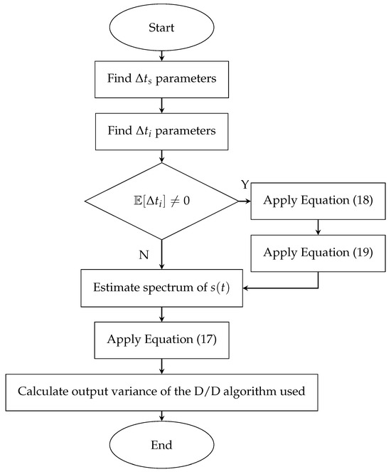
Figure 5.
Block diagram of the application of the proposed method for determining the variance values of delay-related error signals.
A common use case for a “system-on-chip” solution is a measurement chain based on a single microcontroller, in which a built-in A/D converter with an integrated sample-and-hold system is used [37]. This solution provides the possibility of D/D processing using built-in “DSP” instructions [54], which makes it an attractive choice due to its low cost and high capabilities. These advantages are especially appealing to designers of measurement chains. An example of the implementation of the discussed solution is the measurement chain described in [41,43]. The application of the proposed method for estimating the variance of the error signal resulting from delays in the analyzed case focuses on selecting model parameters for the quantities and .
In the case of the measurement process initiation delay parameter, it is necessary to determine which properties of the measurement chain influence the value, particularly relating to the following:
- Whether the measurement chain performs multiple tasks that might be mutually exclusive;
- The typical execution time of the algorithm responsible for detecting the phenomenon that initiates the measurement process;
- The nature of the distribution of the measurement process initiation delay time;
- Whether the S/H system continues to track the input signal after the initiation of A/D processing or whether tracking is performed continuously without interruption.
For the quantity in question, the expected value largely depends on whether the S/H system continuously tracks the input voltage when the A/D processing is not yet active. In practice, this depends on the design of the measurement chain’s software, the hardware capabilities of the microcontroller, and the number of input signals being processed. Most available solutions, such as the one described in [55], offer only one built-in A/D converter with a multiplexed input, which means that simultaneous tracking of multiple input voltages is not feasible. In such a case, the expected value of the parameter will increase by the duration of the tracking time, different from a solution where the tracking process is continuous.
For the parameter , related to fluctuations in the sampling period, the following factors should be analyzed:
- How the processing of subsequent samples from the A/D converter input is initiated;
- The resolution and stability of the clock signal used to measure the sampling time.
In the analyzed case, the method of triggering the A/D converter will have a significant impact on the parameters of the quantity. In solutions similar to [55], there is the possibility of automatic triggering using an internal hardware counter, which is clocked by the system clock. Such a solution ensures very high stability of the A/D converter trigger frequency. For example, according to the datasheet [55], the maximum error value of the clock signal period does not exceed 200ns at a clock frequency of 100MHz. Since the presented datasheet [55] only indicates the limiting value of the clock signal period deviation, it is proposed in this case to follow the guide [30] and assume a uniform distribution of the realization values of the quantity . In the discussed case, the variance value associated with this signal should be determined according to Equation (12), assuming . As shown in [41], for the case discussed, the error signal component related to the analyzed issue is characterized by a negligibly small variance compared to other error signals. However, this situation may differ significantly when the A/D converter is triggered solely in a programmatic manner, as is the case with the platform [56].
The final step of the applied method is to determine how the analyzed error signals related to delays are transferred to the output of the applied D/D algorithm. To achieve this, it is important to understand the transfer function of this algorithm, and such an analysis has been presented in [43], among others. It should be noted that the analyzed error signal is always characterized by a zero expected value and a symmetrical distribution of realization values. This means that the expanded uncertainty associated with subsequent components of this signal can be determined according to the method described in [30], while the resultant expanded uncertainty for this signal can be determined using the methods described in [33,57,58,59,60,61,62,63].
In cases where Wavelet Transform algorithms are applied within the measurement chain—as is the case, for example, with certain short-circuit detection methods [15] and power grid failure detection techniques [14]—the influence of these algorithms on the error signals discussed in this study must be taken into account. For the analysis of the stochastic (non-deterministic) component of the error signal, related to , the method presented in [64] can be employed to calculate the variance of the output error signal. For the deterministic component, related to , the approach proposed in [43] is applicable.
5. Conclusions
This article presents a method for determining the variance of error signals associated with typical delays occurring during A/D processing. The proposed method allows for analytical estimation of the variance parameter of the analyzed error signal, and its results match those obtained by the Monte Carlo method [33]. Therefore, using the proposed method has much lower computational complexity compared to performing simulations. The most important achievements of this work include the following:
- Proposing a uniform and universal model of error signals related to delays;
- Indication of an analytical method for determining the variance value of the discussed error signals for selected parameters of the distribution of delay realizations;
- Indication of the component properties of the error signal related to delays, important from the point of view of analyzing the impact of the D/D processing algorithm on these signals;
- Indication of possible sources and genesis for the discussed error signals;
- Verification of the effectiveness of the proposed method in relation to the Monte Carlo method.
The conducted studies show that the nature of the components of the analyzed error signal is different; hence, despite the uniform method of determining their variance, these components should be analyzed separately. The component associated with the delay in initiating the measurement process on the scale of a single implementation is deterministic, while the component related to sampling period fluctuations is random for each realization.
In the case of a single measurement window, the distribution of the error signal component related to the measurement initiation delay has a “sine” function distribution (the shape of the letter “U”) [44]. On a global scale, however, the distribution of this signal fragment depends on the distribution of the delay parameter. For the component related to sampling period fluctuations, the distribution of its value is identical for each realization of the measurement process (assuming a sufficiently large number of input quantities of the D/D algorithm [30]), and its shape depends on the parameters of this delay-related quantity.
The proposed method provides a very universal tool for analyzing parameters of error signals related to delays and for determining their impact on the uncertainty budget of D/D processing algorithms. Unlike the methods and approaches proposed in [25,26,27,28,29], this method offers a universal and unified approach to the problem, thus complementing the recommendations presented in [30]. Its analytical nature also allows application in cases with different realizations of delay values than those proposed in that study.
It should be emphasized that, for all discussed potential applications of the method presented in this study, the development of an uncertainty budget for the output quantities of the applied measurement chain is of critical importance. In applications related to the detection of the analyzed phenomenon, understanding the potential margin of error is essential. Similarly, in cases involving the estimation of output quantities, such as energy, it is crucial to assess the discrepancy between the obtained and the true value. Due to the time-consuming nature of Monte Carlo simulations and the lack of appropriate analytical error models, this aspect is often neglected. The authors therefore hope that the proposed method will find practical applications across various domains.
Analyzing this work, one can also notice a significant disadvantage of the proposed method: the necessity for analytical determination of the content of Equation (10). The discussed situation concerns the case in which the distribution of the realization of the quantity or is an atypical distribution for which it is not possible to apply any of the models described in the work. However, the analysis of works such as [21,22,23,24,25,26,27,28,29] allows us to assume that, in typical cases, the proposed models can be successfully applied.
All experiments described in this paper can be independently reproduced for any parameters of the and quantities. The GNU Octave scripts (version 9.4.0 [65]) prepared for this purpose are publicly available in the repository [50].
Author Contributions
Data curation, Ł.D.; formal analysis, M.K. and J.R.; funding acquisition, M.K.; investigation, Ł.D.; methodology, M.K. and Ł.D.; project administration, M.K.; resources, Ł.D.; software, Ł.D.; supervision, J.R.; validation, M.K. and J.R.; writing—original draft, Ł.D.; writing—review and editing, M.K. and J.R. All authors have read and agreed to the published version of the manuscript.
Funding
This research was partially funded by the Rector of Silesian University of Technology, grant number 05/020/RGJ25/0094.
Data Availability Statement
All data related to the simulation experiments supporting the conclusions of this article can be replicated using the scripts provided on GitHub [50].
Conflicts of Interest
The authors declare no conflicts of interest.
Abbreviations
The following symbols and abbreviations are used in this manuscript:
| List of Symbols | |
| Measurement chain input quantity | |
| Voltage representation of the | |
| Digital representation of the | |
| N | Number of input quantities of the used DSP algorithm |
| Sampling period | |
| Sampling frequency | |
| Initiation of the measurement process in the ideal situation | |
| Delay of the measurement process initiation | |
| The difference in the processing time of the i-th signal sample | |
| Course of the a quantity in the ideal case | |
| Course of the a quantity in the real case |
| Error signal of the a quantity caused by phenomenon b | |
| Amplitude of the k-th harmonic of the a signal | |
| Phase of the k-th harmonic of the a signal | |
| Pulsation of the k-th harmonic of the a signal | |
| Variance of the a signal | |
| Abbreviations | |
| A/A | Analog-to-analog |
| A/D | Analog-to-digital converter |
| D/D | Digital-to-digital |
| DFT | Discrete Fourier Transform |
| DSP | Digital signal processing |
| S/H | Sample-and-hold |
| WT | Wavelet Transform |
Appendix A
Below are the derivations for the dependencies described in Equations (11)–(16). For clarity, it is assumed that the variance of the signal is determined as follows:
where corresponds to the constant pulsation of this signal (equivalent to the quantity ), corresponds to the constant phase shift (equivalent to the quantity ), and the symbol denotes the time difference between the ideal and real cases (equivalent to the quantities and ). By definition [39,45], the variance of the signal presented in Equation (A1) is as follows:
Hence, the square of this signal is given by the following:
First, we consider the contribution of the variable t to the expression . Assuming that this variable can take any values from the range , we obtain the following:
which follows from the property that for . Then, taking into account the quantity , one obtains the following:
Finally, we calculate the value of the expression :
which follows from the property that for . Finally, we obtain the following:
Appendix A.1. The Case with Uniform Distribution
Therefore, calculating
we obtain the following:
Hence, finally,
Appendix A.2. The Case of Normal Distribution
For Equation (A7), assuming that and substituting , we obtain the following:
Hence,
Further, for simplicity, by substituting , we obtain
where, after expansion
we obtain
while knowing that [66]
After substituting into the above dependencies, we obtain the following:
Therefore,
Hence, finally,
Appendix A.3. The Case of the Gamma Distribution
For , where G denotes the “Gamma” distribution, in Equation (A7), after substituting , we obtain
where
is the probability density function of the Gamma distribution, and the characteristic function of the “Gamma” distribution is described by the following equation [67]:
where, in the analyzed case, the real part of this function is important. Therefore,
where [68]
Hence, finally,
References
- Agarwal, S.; Sharma, S.; Rahman, M.H.; Vranckx, S.; Maiheu, B.; Blyth, L.; Janssen, S.; Gargava, P.; Shukla, V.K.; Batra, S.; et al. Air quality forecasting using artificial neural networks with real time dynamic error correction in highly polluted regions. Sci. Total Environ. 2020, 735, 139454. [Google Scholar] [CrossRef] [PubMed]
- Volosnikov, A.S. Measurement System Based on Nonrecursive Filters with the Optimal Correction of the Dynamic Measurement Error. Meas. Tech. 2023, 65, 720–728. [Google Scholar] [CrossRef]
- Roj, J. Estimation of the artificial neural network uncertainty used for measurand reconstruction in a sampling transducer. IET Sci. Meas. Technol. 2014, 8, 23–29. [Google Scholar] [CrossRef]
- Mallat, S. A Wavelet Tour of Signal Processing, 3rd ed.; Academic Press: Cambridge, MA, USA, 2008. [Google Scholar]
- Addison, P.S. The Illustrated Wavelet Transform Handbook: Introductory Theory and Applications in Science, Engineering, Medicine and Finance, 2nd ed.; CRC Press: Boca Raton, FL, USA, 2017. [Google Scholar]
- Akujuobi, C.M. Wavelets and Wavelet Transform Systems and Their Applications; Springer: Berlin/Heidelberg, Germany, 2022. [Google Scholar]
- Durak, L.; Arikan, O. Short-time Fourier transform: Two fundamental properties and an optimal implementation. IEEE Trans. Signal Process. 2003, 51, 1231–1242. [Google Scholar] [CrossRef]
- Alegria, F. Using digital methods in active power measurement. Acta IMEKO 2023, 12, 1–8. [Google Scholar] [CrossRef]
- Pandey, S. Analog Multiplier Based Single Phase Power Measurement. J. Electr. Electron. Syst. 2016, 5, 2332-0796. [Google Scholar] [CrossRef]
- Unser, M.; Aldroubi, A. A review of wavelets in biomedical applications. Proc. IEEE 1996, 84, 626–638. [Google Scholar] [CrossRef]
- Hasan, O. Automatic detection of epileptic seizures in EEG using discrete wavelet transform and approximate entropy. Expert Syst. Appl. 2009, 36, 2027–2036. [Google Scholar] [CrossRef]
- Yan, R.; Gao, R.X.; Chen, X. Wavelets for fault diagnosis of rotary machines: A review with applications. Signal Process. 2014, 96, 1–15. [Google Scholar] [CrossRef]
- Siddique, M.F.; Ahmad, Z.; Ullah, N.; Kim, J. A Hybrid Deep Learning Approach: Integrating Short-Time Fourier Transform and Continuous Wavelet Transform for Improved Pipeline Leak Detection. Sensors 2023, 23, 8079. [Google Scholar] [CrossRef]
- Liu, Z.; Zhao, Z.; Huang, G.; Wang, F.; Wang, P.; Liang, J. Power Grid Faults Diagnosis Based on Improved Synchrosqueezing Wavelet Transform and ConvNeXt-v2 Network. Electronics 2025, 14, 388. [Google Scholar] [CrossRef]
- Altaie, A.S.; Abderrahim, M.; Alkhazraji, A.A. Transmission Line Fault Classification Based on the Combination of Scaled Wavelet Scalograms and CNNs Using a One-Side Sensor for Data Collection. Sensors 2024, 24, 2124. [Google Scholar] [CrossRef] [PubMed]
- Yan, S.; Gu, Z.; Park, J.H.; Xie, X.; Sun, W. Distributed Cooperative Voltage Control of Networked Islanded Microgrid via Proportional-Integral Observer. IEEE Trans. Smart Grid 2024, 15, 5981–5991. [Google Scholar] [CrossRef]
- STMicroelectronics. Application Note AN1636; STMicroelectronics: Geneva, Switzerland, 2003; Available online: https://www.st.com/resource/en/application_note/an1636-understanding-and-minimising-adc-conversion-errors-stmicroelectronics.pdf (accessed on 30 May 2025).
- Arpaia, P.; Baccigalupi, C.; Martino, M. Metrological characterization of high-performance delta-sigma ADCs. In Proceedings of the 2018 IEEE International Instrumentation and Measurement Technology Conference (I2MTC), Houston, TX, USA, 14–17 May 2018; IEEE: Piscataway, NJ, USA, 2018; pp. 1–6. [Google Scholar] [CrossRef]
- Topór-Kaminski, T.; Jakubiec, J. Uncertainty modelling method of data series processing algorithms. In Proceedings of the 10th International Symposium on Development in Digital Measuring Instrumentation and 3rd Workshop on ADC Modelling and Testing, IMEKO, Naples, Italy, 17–18 September 1998; Volume 2, pp. 631–636. [Google Scholar]
- Baker, B.C. Optimize Your SAR ADC Design; Texas Instruments Inc.: Dallas, TX, USA, 2019. [Google Scholar]
- Jakubiec, J. Błędy i Niepewności Danych w Systemie Pomiarowo-Sterującym; Wydawnictwo Politechniki Śląskiej: Gliwice, Poland, 2010. (In Polish) [Google Scholar]
- Wymysło, M. Badanie związków między błędami opóźnień a innymi błędami w systemie pomiarowo-sterującym w oparciu o definicję współczynnika korelacji. Przegląd Elektrotechniczny 2016, 92, 217–220. (In Polish) [Google Scholar] [CrossRef]
- Wymysło, M. Współbieżna realizacja zadań programowych jako przyczyna powstawania opóźnień w systemie pomiarowo-sterującym. Zesz. Nauk. Wydział Elektrotechniki Autom. Politech. Gdańskiej 2016, 49, 129–132. (In Polish) [Google Scholar]
- Wymysło, M.; Jakubiec, J. Przedziałowa postać wyniku pomiaru jako podstawa wyrażania niedokładności w systemach pomiarowo-sterujących. Zesz. Nauk. WydziałU Elektrotechniki Autom. Politech. Gdańskiej 2018, 59, 73–78. (In Polish) [Google Scholar] [CrossRef]
- Zakharov, I.P.; Vodotyka, S.V.; Shevchenko, E.N. Methods, Models, and Budgets for Estimation of Measurement Uncertainty During Calibration. Meas. Tech. 2011, 54, 387–399. [Google Scholar] [CrossRef]
- Rovera, G.D.; Siccardi, M.; Römisch, S.; Abgrall, M. Time Delay Measurements: Estimation of the Error Budget. Metrologia 2019, 56, 035004. [Google Scholar] [CrossRef]
- Huang, Z.G.; Qiao, C.J.; Ma, C.; Zhao, S. The Analysis and Correction of Time-Delay in the Precise Acoustic Measurement System. Appl. Mech. Mater. 2013, 333–335, 236–242. [Google Scholar] [CrossRef]
- Choi, M.; Choi, J.; Chung, W.K. State estimation with delayed measurements incorporating time-delay uncertainty. IET Control Theory Appl. 2012, 6, 2351–2361. [Google Scholar] [CrossRef]
- Tarasov, V.N. Mathematical Model of Delay Based on a System with Gamma Distribution. Phys. Wave Process. Radio Syst. 2021, 24, 62–67. [Google Scholar] [CrossRef]
- Joint Committee for Guides in Metrology. Evaluation of Measurement Data—Guide to the Expression of Uncertainty in Measurement; JCGM: Sèvres, France, 2008; Available online: https://www.bipm.org/documents/20126/2071204/JCGM_100_2008_E.pdf (accessed on 30 May 2025).
- Laplante, P.A. The certainty of uncertainty in real-time systems. IEEE Instrum. Meas. Mag. 2004, 7, 44–50. [Google Scholar] [CrossRef]
- Bandyszak, T.; Weyer, T.; Daun, M. Uncertainty Theories for Real-Time Systems. In Handbook of Real-Time Computing; Tian, Y., Levy, D.C., Eds.; Springer Nature: Berlin/Heidelberg, Germany, 2022; pp. 99–132. [Google Scholar]
- Joint Committee for Guides in Metrology. Evaluation of Measurement Data—Propagation of Distributions Using a Monte Carlo Method; JCGM: Sèvres, France, 2008; Available online: https://www.bipm.org/documents/20126/2071204/JCGM_101_2008_E.pdf (accessed on 30 May 2025).
- Janssen, H. Monte-Carlo based uncertainty analysis: Sampling efficiency and sampling convergence. Reliab. Eng. Syst. Saf. 2013, 109, 123–132. [Google Scholar] [CrossRef]
- Saleh, R.; Wilton, S.; Mirabbasi, S.; Hu, A.; Greenstreet, M.; Lemieux, G.; Pande, P.P.; Grecu, C.; Ivanov, A. System-on-chip. Proc. IEEE 2006, 94, 1050–1069. [Google Scholar] [CrossRef]
- Renesas Electronics Corporation. Application Note AN-815—Understanding Jitter Units; Renesas Electronics Corporation: Tokyo, Japan, 2020; Available online: https://www.renesas.com/en/document/apn/815-understanding-jitter-units (accessed on 30 May 2025).
- Reay, D.S. Digital Signal Processing Using the ARM Cortex M4; John Wiley & Sons: Hoboken, NJ, USA, 2015. [Google Scholar]
- Jakubiec, J.; Roj, J. Error Analysis of Analytical and Neural Real-Time Reconstruction of Analog Signals; Wydawnictwo Politechniki Śląskiej: Gliwice, Poland, 2024. [Google Scholar] [CrossRef]
- Oppenheim, A.V.; Willsky, A.S.; Nawab, S.H. Signals & Systems, 2nd ed.; Pearson: London, UK, 2013. [Google Scholar]
- Ruhm, K.H. Deterministic, Nondeterministic Signals; Institute for Dynamic Systems and Control: Zurich, Switzerland, 2008. [Google Scholar]
- Kampik, M.; Roj, J.; Dróżdż, L. Error Model of a Measurement Chain Containing the Discrete Wavelet Transform Algorithm. Appl. Sci. 2024, 14, 3461. [Google Scholar] [CrossRef]
- Dróżdż, L.; Roj, J. Origin and properties of own error signals of the discrete wavelet transform algorithms. Int. J. Electron. Telecommun. 2024, 70, 643–648. [Google Scholar] [CrossRef]
- Kampik, M.; Roj, J.; Dróżdż, L. Estimation of the resultant expanded uncertainty of the output quantities of the measurement chain using the discrete wavelet transform algorithm. Appl. Sci. 2024, 14, 3691. [Google Scholar] [CrossRef]
- Horalek, V. Analysis of basic probability distributions, their properties and use in determining type B evaluation of measurement uncertainties. Measurement 2013, 46, 16–23. [Google Scholar] [CrossRef]
- Grimmett, G.; Stirzaker, D. Probability and Random Processes, 4th ed.; Oxford University Press: Oxford, UK, 2020. [Google Scholar]
- Kuo, H.H. White Noise Distribution Theory; CRC Press: Boca Raton, FL, USA, 2018. [Google Scholar] [CrossRef]
- Oppenheim, A.V.; Schafer, R.W. Discrete-Time Signal Processing, 3rd ed.; Pearson: London, UK, 2009. [Google Scholar]
- Proakis, J.G.; Manolakis, D.G. Digital Signal Processing: Principles, Algorithms and Applications, 5th ed.; Pearson: London, UK, 2021. [Google Scholar]
- Jakubiec, J.; Konopka, K. The error based model of a single measurement result in uncertainty calculation of the mean value of series. In Proceedings of the Problems and Progress in Metrology: PPM’15, Gliwice, Poland, 7–10 June 2015; Volume 20, pp. 75–78. [Google Scholar]
- Dróżdż, L. Time Related Error Parameters Estimation Example on GitHub. 2025. Available online: https://github.com/Kuszki/Octave-Uncertainty-TREU-Example (accessed on 30 May 2025).
- Ahmad, K.A. Wavelet Packets and Their Statistical Applications; Springer: Singapore, 2018. [Google Scholar]
- Averbuch, A.Z.; Neittaanmäki, P.; Zheludev, V.A. Spline and Spline Wavelet Methods with Applications to Signal and Image Processing; Springer: Berlin/Heidelberg, Germany, 2019; Volume 3. [Google Scholar]
- Wang, J. On Spline Wavelets. In Wavelets and Splines; Chen, G., Lai, M.-J., Eds.; Nashboro Press: Des Peres, MO, USA, 2006; pp. 456–483. [Google Scholar]
- ARM Limited. CMSIS-DSP—Embedded Compute library for Cortex-M and Cortex-A. 2024. Available online: https://arm-software.github.io/CMSIS-DSP (accessed on 30 May 2025).
- STMicroelectronics. Datasheet DS10314; STMicroelectronics: Geneva, Switzerland, 2017; Available online: https://www.st.com/resource/en/datasheet/stm32f411ce.pdf (accessed on 30 May 2025).
- Atmel. ATmega32/L Datasheet; Atmel: San Jose, CA, USA, 2011; Available online: https://ww1.microchip.com/downloads/en/DeviceDoc/doc2503.pdf (accessed on 30 May 2025).
- Kampik, M.; Roj, J.; Dróżdż, L. A Method for Estimating the Resultant Expanded Uncertainty Value Based on Interval Arithmetic. Appl. Sci. 2024, 14, 7334. [Google Scholar] [CrossRef]
- Koliander, G.; El-Laham, Y.; Djurić, P.M.; Hlawatsch, F. Fusion of probability density functions. Proc. IEEE 2022, 110, 404–453. [Google Scholar] [CrossRef]
- Zhang, Z.; Wang, J.; Jiang, C.; Huang, Z.L. A new uncertainty propagation method considering multimodal probability density functions. Struct. Multidiscip. Optim. 2019, 60, 1983–1999. [Google Scholar] [CrossRef]
- Dieck, R.H. Measurement Uncertainty: Methods and Applications; ISA: Singapore, 2017. [Google Scholar]
- Yang, L.; Guo, Y. Combining pre-and post-model information in the uncertainty quantification of non-deterministic models using an extended Bayesian melding approach. Inf. Sci. 2019, 502, 146–163. [Google Scholar] [CrossRef]
- Urbanski, M.K.; Wąsowski, J. Fuzzy approach to the theory of measurement inexactness. Measurement 2003, 34, 67–74. [Google Scholar] [CrossRef]
- Dróżdż, L. Reductive Interval Arithmetic Method Application Example on GitHub. 2024. Available online: https://github.com/Kuszki/Octave-Uncertainty-RIA-Example (accessed on 30 May 2025).
- Roj, J.; Dróżdż, L. Propagation of Random Errors by the Discrete Wavelet Transform Algorithm. Electronics 2021, 10, 764. [Google Scholar] [CrossRef]
- Eaton, J.W. GNU Octave Official Website. 2024. Available online: https://octave.org (accessed on 30 May 2025).
- Osgood, B. The Fourier Transform and Its Applications; Stanford University: Stanford, CA, USA, 2007. [Google Scholar]
- Tassaddiq, A.; Qadir, A. Fourier Transform and Distributional Representation of the Generalized Gamma Function with Some Applications. Appl. Math. Comput. 2011, 218, 1084–1088. [Google Scholar] [CrossRef]
- Chaudhry, M.A.; Qadir, A. Fourier Transform and Distributional Representation of the Gamma Function Leading to Some New Identities. Int. J. Math. Math. Sci. 2004, 2004, 2091–2096. [Google Scholar] [CrossRef]


Disclaimer/Publisher’s Note: The statements, opinions and data contained in all publications are solely those of the individual author(s) and contributor(s) and not of MDPI and/or the editor(s). MDPI and/or the editor(s) disclaim responsibility for any injury to people or property resulting from any ideas, methods, instructions or products referred to in the content. |
© 2025 by the authors. Licensee MDPI, Basel, Switzerland. This article is an open access article distributed under the terms and conditions of the Creative Commons Attribution (CC BY) license (https://creativecommons.org/licenses/by/4.0/).