A Robust Low-Carbon Optimal Dispatching Method for Power System Distribution Based on LCA Carbon Emissions

Abstract

Under the dual carbon goal, in order to promote the consumption of new energy and reduce carbon emissions in power systems, this paper proposes a new distributed robust low-carbon optimization scheduling method for power systems based on LCA carbon emissions. Firstly, the carbon emissions of energy consumption in the power system are calculated based on the LCA method; secondly, a distributed robust optimization scheduling model is established with the goal of minimizing carbon emissions and economic costs. The model is linearly solvable through the description of uncertain parameters and the transformation of the model. Finally, the optimization results of the example scenario indicate that the distributed robust low-carbon optimization scheduling method based on LCA carbon emissions can effectively reduce carbon emissions and costs compared to traditional methods, providing theoretical support for the new low-carbon optimization strategy of power systems.

1. Introduction

With the continuous promotion of the “dual-carbon” goal, the construction of a new power system with new energy as the main body has become an inevitable trend in the development of China’s power system. The new power system oriented to the dual-carbon goal relies on digital technology, integrates the source, network, load, and storage resources, and proposes a new power system construction plan that coordinates and interacts with the source, network, load, and storage [1], which has become a hot spot of research nowadays.

Most of the studies still focus on system optimization to address the low-carbon emission reduction needs of power systems. Zhang X et al. [2] optimize the scheduling of multi-energy systems by ladder light robust optimization, Zihang M et al. [3] optimize the system scheduling by using the demand response model and the reward and punishment ladder carbon trading model, and Babahammou R H et al. [4] optimize the carbon emission reduction by using solar energy to produce hydrogen to provide power for the gas turbine. Solar energy can also improve the operational efficiency of the power system in a certain environment [5]. In addition, with the gradual maturation and promotion of carbon capture technology, the use of carbon capture devices for low-carbon optimization in power systems is gradually increasing, such as combining carbon capture technology with virtual power plants [6], using energy storage and carbon capture technology for joint peak shifting [7], or low-carbon and economically optimal scheduling under carbon capture technology [8,9,10]. However, due to technical reasons and economic costs, the application of carbon capture devices in power systems is relatively complex [11], and further research is needed. At the same time, due to the gradual formation of the carbon trading market, the study of carbon tax credits and carbon trading as an emission reduction measure has been increasing, and the impact of carbon trading on carbon emission reduction in the power system has been studied through the coupling situation of the electric carbon market [12,13,14]. Research on carbon emission calculation [15] is also increasing, and multi-objective power system optimal scheduling for calculating carbon emissions has also appeared [16]. Most of the above carbon emission reduction studies focus on the system optimization level, combined with market trading or carbon capture technology, but are relatively absent at the carbon emission calculation level. Most of the current carbon emission calculations are based on the calculation of current power or energy flow in the power grid [17,18], without considering the complexity of the new power system, that the system in the operation process of the source, network, and storage will produce carbon emissions, and that market trading is another form of carbon emissions on the flow, so describing the system emission reduction effect needs to be strongly verified by carbon accounting.

Distributionally robust optimization (DRO) is an important method for solving uncertainty problems, which has been heavily used in system prediction [19], capacity allocation [20], optimal scheduling [21,22], and other studies. Wind and light outputs and loads in the new power system have uncertainty, but the historical empirical data can be known to exist in an unknown probability distribution, so the combination of chance constraints and robust optimization overcomes the shortcomings of robust optimization being too conservative and chance constraints being too sensitive to parameter changes. Therefore, this paper establishes a distributional robust optimization scheduling model with the objective of minimizing the economic cost, taking into account the carbon emission of the whole life cycle of the system, and verifies the validity of the model, taking into account the source and load uncertainties.

2. LCA Carbon Emissions Assessment

2.1. Carbon Emission Analysis Methodology Based on Life Cycle Assessment

Life Cycle Assessment (LCA) is an international standard method for systematically and quantitatively describing various resources, energy consumption, and environmental emissions during the life cycle of a product and evaluating its environmental impact. Currently, LCA theory is mainly applied in the field of construction engineering, but it is also involved in the carbon emission measurement of power systems, such as the introduction of LCA concepts in the low-carbon optimization of integrated energy systems [23].

In the most widely used LCA technical framework, target and scope determination is the first step of LCA, and its determination directly affects the accuracy of the subsequent assessment results. In this paper, the energy and equipment cycle LCA carbon emission analysis method [24] is adopted to comprehensively analyze the energy carbon emissions of coal and natural gas-based cycles in the new power system, and to consider the carbon emissions generated by different equipment in the various stages of production, construction, operation, and decommissioning so as to carry out a full-life-cycle measurement of the carbon emissions of the whole system.

2.2. Systematic Carbon Life Cycle Assessment

LCA carbon emissions from the energy cycle come mainly from energy extraction, energy transportation, power generation operations, and exhaust gas treatment. The energy sources considered in this paper include coal and gas energy purchased from energy markets.

Carbon dioxide emissions from coal-fired units in the production of electricity come mainly from the process of excavation and cleaning, handling and transportation of coal, and combustion for power generation, as shown in the formula below:

$${\delta }_{coal}={\delta }_{pc}+{\delta }_{tc}+{\delta }_{uc}$$

(1)

$${\delta }_{pc}=I_{cp}{\eta }_{cp}{Q}_{pc}(1+\alpha +\beta )$$

(2)

$${\delta }_{tc}=Q_{tc}{M}_{coal}{D}_{tc}$$

(3)

$${\delta }_{uc}=I_{uc}{Q}_{uc}$$

(4)

In the formula, ${\delta }_{\mathrm{coal}}$ is the carbon emission factor per unit of electricity for the coal production part of the energy cycle; ${\delta }_{\mathrm{pc}}$ is the carbon emission factor per kilowatt-hour of coal production; ${\delta }_{\mathrm{tc}}$ is a coefficient of carbon emissions per unit of electricity during coal transportation; ${\delta }_{\mathrm{uc}}$ is the coefficient of carbon emissions per unit of electricity produced by the coal-fired power generation chain; $I_{\mathrm{cp}}$ is the unit loss of coal; ${\eta }_{\mathrm{cp}}$ is the conversion efficiency of coal; $Q_{\mathrm{pc}}$ is the carbon intensity of coal production; $\alpha$ is the rate of power loss per unit due to spontaneous combustion of raw coal; $\beta$ is the unit power loss rate due to raw coal washing; $Q_{\mathrm{tc}}$ is the carbon intensity of the coal transportation process; $M_{\mathrm{coal}}$ is the transportation of coal; $D_{tc}$ is the distance that coal is transported; $I_{\mathrm{uc}}$ is the unit coal consumption in the power generation chain, which is related to the power generated; and $Q_{\mathrm{uc}}$ is the carbon emission intensity per unit of coal consumed in the power generation process.

Similarly, the carbon emission factor of natural gas energy in the integrated energy system ${\delta }_g$ can be obtained. Then, the carbon emission calculation formulas for coal-fired and gas-fired units are shown below:

$$E_m={\delta }_{coal}{\displaystyle {\sum }_{t=1}^T{P}_{coal,t}}$$

(5)

$$E_g={\delta }_g{\displaystyle {\sum }_{t=1}^T{P}_{\mathrm{g},t}}$$

(6)

In the formula, $E_m$ and $E_{\mathrm{g}}$ are the actual carbon emissions from coal-fired and gas-fired units, respectively; $P_{coal,t}$ and $P_{\mathrm{g},t}$ a is the output of coal-fired and gas-fired units in time period t; and ${\delta }_{coal}$ and ${\delta }_{\mathrm{g}}$ are coal and gas-fired carbon emission factors.

System LCA carbon emissions are made up of a combination of energy LCA carbon emissions from both coal-fired and gas-fired sources.

3. System Modeling

3.1. Objective Function

(1)

The cost objective:

$$\min C_{ss}+C_N+C_{ab}+C_{el}+C_{tr}+C_{dr}$$

(7)

In the formula, $C_{\mathrm{ss}}$ is the startup and shutdown cost of coal-fired and gas-fired units; $C_{\mathrm{N}}$ is the cost of wind power output for the new power system; $C_{\mathrm{ab}}$ is the cost of wind and light abandonment; $C_{\mathrm{el}}$ is the operating cost of electrochemical energy storage; $C_{\mathrm{tr}}$ is the cost of carbon trading; and $C_{\mathrm{dr}}$ is load cutting costs.

$$\begin{array}{l}{C}_{ss}={\displaystyle {\sum }_{t=2}^T{\displaystyle {\sum }_i^{I_m}\left\{\left[u_{i,t}^m\left(u_{i,t}^m-u_{i,t-1}^m\right)\right]c_{q,m}+\left[\left(1-u_{i,t}^m\right)\left(u_{i,t-1}^m-u_{i,t}^m\right)\right]c_{s,m}\right\}}}\\ +{\displaystyle {\sum }_{t=2}^T{\displaystyle {\sum }_i^{I_g}\left\{\left[u_{i,t}^g\left(u_{i,t}^g-u_{i,t-1}^g\right)\right]c_{q,g}+\left[\left(1-u_{i,t}^g\right)\left(u_{i,t-1}^g-u_{i,t}^g\right)\right]c_{s,g}\right\}}}\end{array}$$

(8)

$$C_N={\displaystyle {\sum }_t^T\left(P_{w,t}{c}_w+P_{pv,t}{c}_{pv}\right)}$$

(9)

$$C_{ab}={\displaystyle {\sum }_t^T\left[c_{ab}^{pv}\left(P_t^{pv\max }-P_{pv,t}\right)+c_{ab}^w\left(P_t^{w\max }-P_{w,t}\right)\right]}$$

(10)

$$C_{el}={\displaystyle {\sum }_t^T{\displaystyle {\sum }_i^{lh}\left(c_{ch,el}{P}_{el,t}^{ch,l}{u}_{el,t}^{ch,l}+c_{dis,el}{P}_{el,t}^{dis,l}{u}_{el,t}^{dis,l}\right)}}$$

(11)

$$C_{tr}={\displaystyle {\sum }_n{E}_{tr,n}}{c}_{tr,n}$$

(12)

$$C_{dr}={\displaystyle {\sum }_m{L}_{t,m}^{cur}}{c}_m^{cur}$$

(13)

In the formula, $c_{q,m}$ and $c_{s,m}$ are the unit startup and shutdown costs of coal-fired units, respectively, $c_{q,g}$ and $c_{s,g}$ are the unit startup and shutdown costs for gas-fired units, respectively; $c_w$ and $c_{pv}$ are the cost of electricity generation per unit of power for wind and PV, respectively; $P_{w,t}$ and $P_{pv,t}$ are the wind and photovoltaic outputs at time period t, respectively; $c_{ab}^{pv}$ and $c_{ab}^w$ denote the penalty cost per unit of power forgone for light and wind, respectively; $P_t^{pv\max }$ and $P_t^{w\max }$ denote the maximum generation power of PV and wind power in time period t; $P_{el,t}^{ch,l}$ and $P_{el,t}^{ch,l}$ are the charging and discharging power of the electrochemical energy storage at time period t, respectively, $c_{ch,el}$ and $c_{dis,el}$ are the cost of charging and discharging per unit power of electrochemical energy storage, respectively; $E_{tr,n}$ is the amount of carbon traded in the nth segment; $c_{tr,n}$ is the carbon trading price for segment n; $L_{t,m}^{cur}$ is the load curtailment for the mth order tariff in time period t; and $c_m^{\mathrm{cur}}$ is the tariff of the mth order as Figure 1 shown.

In order to more effectively reduce actual carbon emissions, the ladder carbon trading model divides the traditional carbon trading model into multiple trading zones based on actual carbon emissions. When the actual carbon emissions of the power generation enterprises are lower than the carbon quota, they can gain revenue by selling the remaining carbon quota, which can improve the enthusiasm of the power generation enterprises to reduce carbon emissions; when the actual carbon emissions of the power generation enterprises are higher than the carbon quota, they need to purchase the carbon emission rights, which increases the extra cost. The cost and benefit model of carbon trading is established as follows:

$$f_{ce}=\left\{\begin{array}{c}-\left[\left(E_p-2d\right)-E_c\right]w_{e,3}-d\left(w_{e,2}+w_{e,1}\right),E_c\le E_p-2d\\ -\left[\left(E_p-d\right)-E_c\right]w_{e,2}-d{w}_{e,1},E_p-2d\le E_c\le E_p-d\\ -\left(E_p-E_c\right)w_{e,1},E_p-d\le E_c\le E_p\\ \left(E_p-E_c\right)c_{e,1},E_p\le E_c\le E_p+d\\ \left[\left(E_p-d\right)-E_c\right]c_{e,2}+d{c}_{e,1},E_p+d\le E_c\le E_p+2d\\ \left[\left(E_p-2d\right)-E_c\right]c_{e,3}+d\left(c_{e,1}+c_{e,2}\right),E_p+2d\le E_c\le E_p+3d\end{array}\right\}$$

(14)

$$E_c={\displaystyle {\sum }_t\left({\delta }_{coal}{P}_{coal,t}+{\delta }_g{P}_{g,t}\right)}$$

(15)

$$W_{e,i}=p_{e,i}\left(1+ir\right),\forall i=1,2,3$$

(16)

$$c_{e,i}=p_{e,i}\left(1+ip\right),\forall i=1,2,3$$

(17)

In the formula, $E_p$ is the amount of carbon allowances; $d$ is carbon emission intervals; $E_c$ is the total carbon emissions for the day; $p_{e,i}$ are the stepped carbon prices traded under different carbon emissions, respectively; $r$ and $p$ are the reward and penalty factors for carbon emissions, respectively; and $W_{e,i}$ and $c_{e,i}$ are the kWh benefit and kWh cost of participating in each tier of carbon trading, respectively.

(2)

Carbon emission target

Another layer of the model’s objective function is to minimize the system’s full life-cycle carbon emissions, that is,

$$\min LCA=E_m+E_g={\delta }_{coal}{\displaystyle {\sum }_{t=1}^T{P}_{coal,t}}+{\delta }_g{\displaystyle {\sum }_{t=1}^T{P}_{g,t}}$$

(18)

Among them, the unit coal consumption $I_{uc}$ and unit gas consumption $I_{ug}$ in the power generation segment in ${\delta }_{coal}$ and ${\delta }_g$ are determined by the power generation with the following equations:

$$I_{uc}=a_i{P}_{coal,t}^2+b_i{P}_{coal,t}+c_i$$

(19)

$$I_{ug}=a_g{P}_{g,t}+c_g$$

(20)

In the formula, $a,b,c$ represent the coefficients of the relationship between coal consumption and generating power, and the coefficients for different units are related to their unit types and unit capacity sizes.

3.2. Restrictive Condition

(1)

Crew constraints

Thermal power units need to satisfy the regulation power constraints, ramp-up constraints, and minimum start/stop time constraints during operation. The coal-fired unit operation is modeled as follows:

$$u_{i,t}^m{P}_{m,i}^{\min }\le P_{i,t}^m\le u_{i,t}^m{P}_{m,i}^{\max }$$

(21)

$$P_{i,t+1}^m-P_{i,t}^m\le u_{i,t}^m{P}_{m,i}^{up}+(1-u_{i,t}^m)P_{m,i}^{\max }$$

(22)

$$P_{i,t}^m-P_{i,t+1}^m\le u_{i,t}^m{P}_{m,i}^{down}+(1-u_{i,t+1}^m)P_{m,i}^{\max }$$

(23)

$${\displaystyle {\sum }_{k=0}^{t_{m,i}^{on}-1}{u}_{i,t+k}^m}\ge \left(u_{i,t}^m-u_{i,t-1}^m\right)\cdot \min \left\{t_{m,i}^{on},T-t+1\right\}$$

(24)

$${\displaystyle {\sum }_{k=0}^{t_{m,i}^{off}-1}(1-u_{i,t+k}^m)}\ge \left(u_{i,t-1}^m-u_{i,t}^m\right)\cdot \min \left\{t_{m,i}^{off},T-t+1\right\}$$

(25)

In the formula,$P_{i,t}^m$ is the generating power of coal-fired unit i at time period t; $P_{m,i}^{\min }$ is the minimum power of coal-fired unit i after flexibility modification; $P_{m,i}^{\max }$ is the maximum power of the coal-fired unit i after flexibility modification; and $P_{m,i}^{down}$ and $P_{m,i}^{up}$ are the downclimb and upclimb power limits for coal-fired flexibility unit i.

$t_{m,i}^{on}$ and $t_{m,i}^{off}$ are the minimum start/stop times for coal-fired flexibility unit i, respectively; $T$ is the total operating period.

Similar to coal-fired units, gas-fired units are modeled as follows:

$$u_{i,t}^g{P}_{g,i}^{\min }\le P_{i,t}^g\le u_{i,t}^g{P}_{g,i}^{\max }$$

(26)

$$P_{i,t+1}^g-P_{i,t}^g\le u_{i,t}^g{P}_{g,i}^{up}+(1-u_{i,t}^g)P_{g,i}^{\max }$$

(27)

$$P_{i,t}^g-P_{i,t+1}^g\le ug{P}_{g,i}^{down}+(1-u_{i,t+1}^g)P_{g,i}^{\max }$$

(28)

$${\displaystyle {\sum }_{k=0}^{t_{g,i}^{on}-1}{u}_{i,t+k}^g}\ge \left(u_{i,t}^g-u_{i,t-1}^g\right)\cdot \min \left\{t_{g,i}^{on},T-t+1\right\}$$

(29)

$${\displaystyle {\sum }_{k=0}^{t_{g,i}^{off}-1}(1-u_{i,t+k}^g)}\ge \left(u_{i,t-1}^g-u_{i,t}^g\right)\cdot \min \left\{t_{g,i}^{off},T-t+1\right\}$$

(30)

In the formula, $P_{i,t}^g$ is the generation power of gas unit i at time period t; $P_{g,i}^{\min }$ is the minimum power of the gas unit i after flexibility modification; $P_{g,i}^{down}$ and $P_{g,i}^{up}$ is the downclimb and upclimb power limit for gas-flexibility unit i; $t_{g,i}^{on}$ and $t_{g,i}^{off}$ are the minimum start/stop times for gas-fired flexibility units, respectively; and $T$ is the total operating period.

(2)

System power constraints

The sum of thermal unit output, wind power output, storage output, and purchased power for each time period within the power system must be equal to the current time period’s electricity load, i.e.,

$${\displaystyle {\sum }_i^{I_m}{P}_{i,t}^m}+{\displaystyle {\sum }_i^{I_g}{P}_{i,t}^g}+P_{w,t}+P_{pv,t}+P_{el}+P_{lh,t}=P\_d_t$$

(31)

In the formula, $P_{i,t}^g$ is the generation power of gas unit i at time period t; $P_{i,t}^m$ is the generating power of coal-fired unit i at time period t; $P\_d_t$ is the load of the power system at time period t; $P_{lh,t}$ is the total electricity purchased at time period t; $P_{w,t}$ and $P_{pv,t}$ are the wind and light outputs, respectively; and $P_{el}$ is the electrochemical energy storage output.

(3)

Wind and light output constraints

The maximum wind and light output shall not be exceeded for all time periods:

$$0\le P_{w,t}\le P_{w,t}^{\max }$$

(32)

$$0\le P_{pv,t}\le P_{pv,t}^{\max }$$

(33)

(4)

Electrochemical energy storage constraints

The maximum capacity and power rating of the electrochemical energy storage system are rated, and the capacity state of the system is required to return to the state of the system at that point in time on the previous day prior to the start of the next day’s operation in order to ensure that the system operates properly on the next day.

$$u_{el,t}^{ch}{P}_{el}^{ch,\min }\le P_{el,t}^{ch,g}+P_{el,t}^{ch,l}\le u_{el,t}^{ch}{P}_{el}^{ch,\max }$$

(34)

$$u_{el,t}^{dis}{P}_{\mathrm{el}}^{dis,\min }\le P_{el,t}^{dis,l}\le u_{el,t}^{dis}{P}_{\mathrm{el}}^{dis,\max }$$

(35)

$$u_{el,t}^{ch}+u_{el,t}^{dis}\le 1$$

(36)

$$S_{el,t}^l=S_{el,t-1}^l+{\eta }_{el}\left(P_{el,t}^{ch,g}+P_{el,t}^{ch,l}\right)-{\displaystyle \frac{P_{el,t}^{dis,l}}{{\eta }_{el}}}$$

(37)

$${\beta }_{el}^{\min }{S}_{el}^l\le S_{el,t}^l\le {\beta }_{el}^{\max }{S}_{el}^l$$

(38)

$$S_{el,1}^l=S_{el,24}^l$$

(39)

$$P_{el}^{ch,\min }\le P_{el,t}^{ch,l}\le P_{el}^{ch,\max }$$

(40)

$$P_{\mathrm{el}}^{dis,\min }\le P_{el,t}^{dis,l}\le P_{\mathrm{el}}^{dis,\max }$$

(41)

$$u_{el,t}^{ch}+u_{el,t}^{\mathrm{dis}}=1$$

(42)

In the formula, $u_{el,t}^{ch}$ and $u_{el,t}^{dis}$ are the 0–1 variables for charging and discharging of the electrochemical energy storage system, respectively; $P_{el}^{ch,\min }$ and $P_{el}^{ch,\max }$ are the minimum and maximum charging power of the electrochemical energy storage system, respectively; $P_{el}^{dis,\min }$ and $P_{el}^{dis,\max }$ are the minimum and maximum discharge power of the electrochemical energy storage system, respectively; $P_{el,t}^{ch,g}$ is an electrochemical energy storage system that supplements the electrical energy in the system by purchasing electricity from the larger grid; ${\beta }_{el}^{\min }$ and ${\beta }_{el}^{\max }$ are the minimum and maximum capacity ratios of the electrochemical energy storage system, respectively; and $S_{el,t}^l$ is the stock of electrochemical energy storage at time t.

(5)

Load reduction constraints

$$L_t^{cur}={\displaystyle {\sum }_m{L}_{t,m}^{cur}}$$

(43)

$$0\le L_{t,m}^{cur}\le \left(L_m^{cur,\max }-L_{m-1}^{cur,\max }\right)$$

(44)

In the formula, $L_t^{cur}$ is the total load reduction in time period t; $L_{t,m}^{cur}$ is the actual load reduction in time period t where the load reduction is located in segment m; and $L_m^{cur,\max }$ is the actual load curtailment when load curtailment is carried out in segment m.

(6)

Distributed robust constraint

$$P\left\{{\displaystyle {\sum }_{i\in S_{\mathrm{c}}}{P}_{i,\min }^{\mathrm{h}}+{\displaystyle {\sum }_{i\in S_{\mathrm{g}}}{P}_{i,\min }^{\mathrm{g}}}\le {\displaystyle {\sum }_{i\in S_{\mathrm{c}}}{P}_{i,t}^h+{\displaystyle {\sum }_{i\in S_{\mathrm{g}}}{P}_{i,t}^{\mathrm{g}}+\left({{\rm Y}}_{pv}+{{\rm Y}}_w\right){\xi }_e\le }}}{\displaystyle {\sum }_{i\in S_c}{P}_{i,\max }^h+{\displaystyle {\sum }_{i\in S_{\mathrm{g}}}{P}_{i,\min }^{\mathrm{g}}}}\right\}\ge 1-{\epsilon }_p$$

(45)

$$P\left\{{\displaystyle {\sum }_{i\in S_{cur}}{P}_{i,t}^{d,cur}\le }{\displaystyle {\sum }_{i\in S_{cur}}{P}_{i,t}^{r,cur}}+{\xi }_d\right\}\ge 1-{\epsilon }_d$$

(46)

In the formula, $S_{\mathrm{c}}$ and $S_g$ are the sets of coal-fired and gas-fired units used for real-time adjustment of output, respectively; $1-{\epsilon }_p$ and $1-{\epsilon }_d$ are the confidence intervals that the system operation scheme satisfies the constraint (31), respectively; and $P_{i,t}^{r,cur}$ is the actual amount of load reduction through load curtailment.

Figure 1. Load reduction ladder cost indication.

Figure 1. Load reduction ladder cost indication.

4. Distributed Robust Optimization

4.1. Uncertainty Parameterization

Since wind and light output and load uncertainties follow empirical distributions extracted from historical forecast error data, fuzzy sets are built to obtain the potential true distribution of the uncertainty set, which contains the worst case of the true distribution, by combining the theory of robust optimization on the basis of stochastic optimization theory. Compared with stochastic planning traditional robust optimization, (DRO) bridges the gap between data and decision making and statistics and optimization frameworks and also inherits the solvability of robust optimization and the flexibility of stochastic planning. The fuzzy set uses the Wasserstein distance $W\left(P_N,P\right)$ to describe the distance between the empirical distribution $P_N$ and the true distribution $P$ [25]:

$$W\left(P_N,P\right)={\left[\inf {\displaystyle \int \rho {\left(e_N,e\right)}^{\mathrm{p}}Q\left(d{e}_N,de\right)}\right]}^p$$

(47)

By introducing the Wasserstein distance into the fuzzy set construction, the resulting fuzzy set can be regarded as a sphere with a true distribution $P$ around an empirical distribution $P_N$ and a radius $\theta \ge 0$. The sphere contains all possible true distributions of wind power prediction errors. Then, Wasserstein fuzzy set can be defined as

$$\mathsf{\Gamma }\left(\theta \right)=\left\{P\in P_0\left(R^{T+1}\times \left[S\right]\right)\left|\begin{array}{c}\left[\left(e,v\right),s\right]~P\\ E_p\left[v\left|s\in \left[S\right]\right.\right]\le \theta \\ P\left[\left(e,v\right)\in {\epsilon }_s\left|=\right.S\right]=1\\ P\left[s=S\right]=P_S,s\in \left[S\right]\end{array}\right.\right\}$$

(48)

In the formula, $P_0$ is the set of true distributions.

$S$ is the number of scenes; $v$ is an auxiliary variable; $s$ is a scene variable; $P_S$ is the probability of scenario $S$; and ${\epsilon }_s$ is a support set for scene $S$ and is satisfied:

$${\epsilon }_s=\left\{\left(e,v\right)\in R^{T+1}\left|\overline{\widehat{e}}\le e\le \underset{¯}{\widehat{e}},\rho \left({\widehat{e}}_s,e\right)\le v\right.\right\},s\in \left[S\right]$$

(49)

In the formula, $\overline{\widehat{e}}$ and $\underset{¯}{\widehat{e}}$ are the upper and lower bounds of the wind and light prediction errors, respectively. The prediction errors have different interval ranges at different confidence levels, and ${\widehat{e}}_s$ is the prediction error for scene $S$.

4.2. Model Transformation

(1)

Linear transformation of the objective function

For fixed $y$ and $z$, the computation of the objective function requires finding the worst-case expectation of a linear function of $\xi$ on the Wasserstein sphere $\mathcal{P}$. This problem is equivalent to a cone optimization problem.

$$\underset{P\in P}{\max }{E}^P\left[c^{T}yz\xi \right]$$

(50)

$$\underset{{\lambda }^{\mathrm{o}},s^{\mathrm{o}},{\gamma }^{\mathrm{o}}}{\min }{\lambda }^{\mathrm{o}}\rho +{\displaystyle \frac{1}{N}}{\displaystyle \sum _{i=1}^N{s}_i^o}$$

(51)

$$\mathrm{s}.\mathrm{t}{c}^{T}yz\widehat{\xi }+{\gamma }_i^o\left(h-H\widehat{\xi }\right)\le s_i^o,\forall i\le N$$

(52)

$$‖H{\gamma }_i^o-{yzc‖}_{\ast }\le {\lambda }^{\mathrm{o}}$$

(53)

$${\gamma }_i^o\in R_{+}^{2W},{\lambda }^{\mathrm{o}}\in R_{+}^{2W},s^o\in R_{+}^{2W}$$

(54)

In the formula, ${\parallel ·\parallel }_{*}$ is a pairwise paradigm of $\parallel ·\parallel$.

(2)

Approximate methods for combining Bonferroni and CVaR

If the joint chance constraint involves $K$ linear inequalities, we can decompose the matrix $A\left(y\right)$ and the vector $b\left(x\right)$ as

$$A\left(y\right)={\left[a_1\left(y\right)\dots a_K\left(y\right)\right]}^T$$

(55)

$$B\left(x\right)={\left[b_1\left(x\right)\dots b_K\left(x\right)\right]}^T$$

(56)

Thus, the joint chance constraint is equivalent to

$$\underset{P\in P}{\min }P\left[a_k\left(y\right)\xi \le b_k\left(x\right)\forall k\le K\right]\ge 1-\epsilon$$

(57)

Given a set of constraint tolerance probabilities ${\epsilon }_k\ge 0$ and $k\le K$, and included among these, ${\displaystyle {\sum }_{k=1}^K{\epsilon }_k}=\epsilon$. The original joint chance constraint can be decomposed into a simpler but more conservative k-family independent chance constraint using Bonferroni’s inequality. This is equivalent to approximating the constraint feasible set ${\Omega }_{cc}$ as ${\Omega }_B$, and ${\Omega }_B$ is denoted as follows:

$${\Omega }_B\triangleq \left\{\left(x,Y\right):\underset{P\in P}{\min }P\left[a_k\left(y\right)\xi \le b_k\left(x\right)\forall k\le K\right]\ge 1-{\epsilon }_k\forall k\le K\right\}$$

(58)

Bonferroni’s inequality shows that ${\Omega }_B\subseteq {\Omega }_{cc}$. For ${\Omega }_B$, even if $\rho =0$ is still difficult to solve optimally, it is necessary to approximate the worst-case chance constraints for each individual constraint by the worst-case CVaR constraints. Thus, ${\Omega }_B$ is conservatively approximated:

$${\Omega }_{BC}\triangleq \left\{\left(x,Y\right):\underset{P\in P}{\min }P-CVa{R}_{{\epsilon }_k}\left[a_k\left(y\right)\xi \le b_k\left(x\right)\right]\le 0\forall k\le K\right\}$$

(59)

${\Omega }_{BC}$ constitutes an optimal convex approximation of ${\Omega }_B$ in some sense, and ${\Omega }_{BC}\subseteq {\Omega }_B$. Moreover, if ${\epsilon }_k\le N^{-1}$ exists for all $k\le K$, then ${\Omega }_{BC}\subseteq {\Omega }_B$. ${\Omega }_{BC}$ is equivalent to the following cone optimization form:

$${\lambda }_k\rho +{\displaystyle \frac{1}{N}}{\displaystyle \sum _{i=1}^N{\mathrm{s}}_{ik}\le 0,}\forall k\le K$$

(60)

$${\tau }_k\le {\mathrm{s}}_{ik},\forall i\le N,\forall k\le K$$

(61)

$$a_k\left(y\right){\widehat{\xi }}_i-b_k\left(x\right)+\left({\epsilon }_k-1\right){\tau }_k+{\epsilon }_k{\gamma }_{ik}\left(h-H{\widehat{\xi }}_i\right)\le {\epsilon }_k{\mathrm{s}}_{ik},\forall i\le N,\forall k\le K$$

(62)

$$‖{\epsilon }_{k}H{\gamma }_{ik}-{a_k\left(y\right)‖}_{\ast }\le {\epsilon }_k{\lambda }_k,\forall i\le N,\forall k\le K$$

(63)

$${\gamma }_{ik}\in R_{+}^{2W},\forall i\le N,\forall k\le K$$

(64)

$$\tau \in R^K,\lambda \in R^K,s\in R^{N\times K}$$

(65)

5. Calculus Analysis

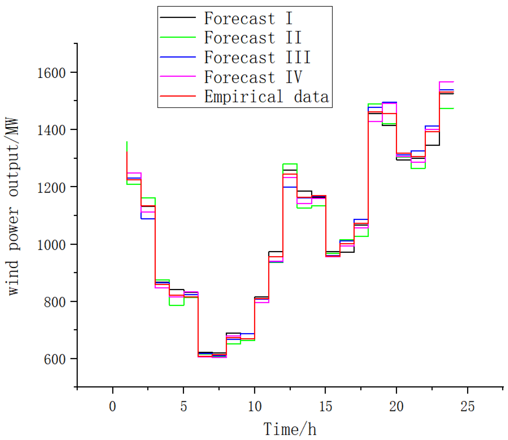
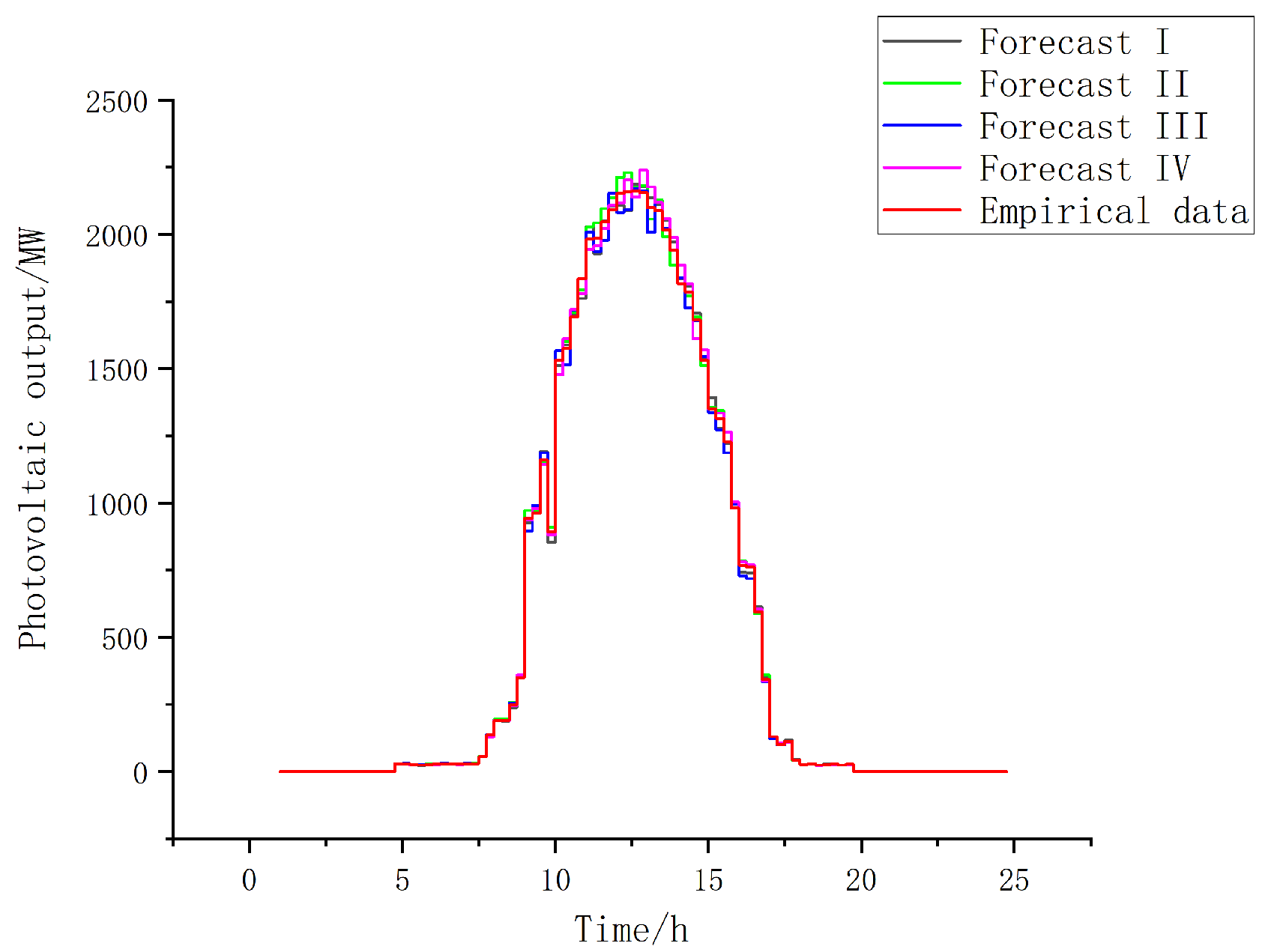
5.1. Example Data

In this paper, a new power system is designed to simulate and verify the model, in which the total capacity of the energy storage system is 600 MWh. The charging and discharging rated power is set to 80 MW. The charging and discharging efficiency is set to 0.95 and the initial value of SOC is set to 30%. The wind power and load are uncertain variables, which are predicted by historical data. In the process of constructing robust distribution models, their prediction errors are generated through a normal distribution. The mean is set to 100 MW, and the standard deviation is set to 1. The coal-fired unit contains twelve coal-fired generators, of which the first seven are conventional power generators, and the last five are flexibility-regulated generators and the gas-fired unit contains four gas turbines, and the specific parameters are shown in

Table 1. Generator set parameter table.

Generators	Maximum Output MW	Minimum Output MW	Coal or Gas Consumption Parameters a	Coal Consumption Parameters b	Coal or Gas Consumption Parameters c
coal burner 1	1000	300	0.0015	0.27	15.23
coal burner 2	1000	300	0.0015	0.27	15.23
coal burner 3	600	180	0.0023	0.274	11.71
coal burner 4	600	180	0.0023	0.274	11.71
coal burner 5	600	180	0.0023	0.274	11.71
coal burner 6	450	135	0.00336	0.293	8.88
coal burner 7	450	135	0.00336	0.293	8.88
coal burner 8	450	135	0.00336	0.293	8.88
coal burner 9	200	70	0.00426	0.321	5.14
coal burner 10	200	70	0.00426	0.321	5.14
coal burner 11	150	45	0.00558	0.332	3.54
coal burner 12	150	45	0.00558	0.332	3.54
gas engine 1	300	80	0.00217	/	6.88
gas engine 2	300	80	0.00217		3.14
gas engine 3	120	50	0.00217		3.14
gas engine 4	120	50	0.00247		2.54
wind turbine	1500	0	/
photovoltaic unit	2000	0

. In Table 1, parameters a, b, c represents a_i, b_i, c_i or a_g, c_g in Formulas (19) and (20). Load reduction segmented price are shown in

Table 2. Load reduction segmented price list.

Load Shedding/MW	Prices/CNY·MWh−1
0–200	250
200–500	360
500–700	430
700–800	550

. Carbon emission trading segment price are shown in

Table 3. Carbon emission trading segment price list.

Carbon Trading Volume/t	Prices/CNY·t−1
$E_{\mathrm{p}}\pm 2000$	40
$E_{\mathrm{p}}\pm 4000$	60
$E_{\mathrm{p}}\pm 6000$	90

.

Since the wind and light output data are predictively modeled using distributional robusts, the predicted wind and light output values for the four scenarios of distributional robusts are compared with the historical empirical data, and the resulting comparison plots are shown below.

From the Figure 2 and Figure 3, it can be seen that the predicted value of the wind and light output data in multiple scenarios is more consistent with the actual empirical distribution data, and it is known that the maximum error of the data is not more than 5%, so the predicted data can be used as the example data to calculate the system to optimize the scheduling.

5.2. Comparative Analysis

(1)

Optimization results

Under the power system set up in this paper, the optimized dispatch output results of the system in a typical working day of 24 h are obtained by considering the whole life cycle carbon emission, demand impact, and distribution robustness of LCA as shown in Figure 4.

From Figure 4 and Figure 5, it can be seen that under the system optimization result aiming at cost minimization, coal-fired units take most of the system output, followed by wind and solar output, while the charging and discharging power of the energy storage part is small. This is because the generation cost of coal-fired units is low, followed by gas-fired units, while the charging and discharging cost of energy storage is relatively high; the load shedding in each time period is more balanced, which can effectively reduce carbon emissions. In 24 h, wind power output is more average, while at 10:00–16:00, due to higher light intensity, the PV (photovoltaic) power is more, so coal-fired and gas-fired units are at the minimum of the day; at 18:00–22:00, load demand peaks, and there is no sunshine, so PV no longer produces power, so the coal-fired units’ output reaches its peak.

In the system, energy storage is used to smooth out the uncertainty of wind and light output, and it can be seen from the uncertainty of wind and light part of the output value and energy storage charging and discharging situation that the charging and discharging of energy storage and the uncertainty of wind and light output have a complementary tendency, and the storage is in a charging state in the midday and afternoon hours due to the greater light intensity, and the energy storage is in a charging state in the wind and light output is more, and in the time of 18:00–22:00, the load demand reaches the peak, wind and light output is insufficient. The energy storage is in the discharging state.

The optimization effects of system load shedding and carbon trading are examined by modifying the model parameters to set up the following different scenarios for comparison:

1:

Carbon trading, load shedding;

2:

Carbon trading, no load shedding;

3:

No carbon trading, load shedding;

4:

No carbon trading, no load shedding.

The results of scene comparison are obtained as shown in

Table 4. Comparison of costs and carbon emissions in different scenarios.

Scenarios	Costs/CNY	Carbon Footprint/t
1	71,317,876.86	134,636.42
2	70,758,017.43	148,848.16
3	66,856,792.55	170,248.98
4	65,987,341.52	181,174.54

:

As shown in Table 4, by comparing Scenario 1 and Scenario 2, it can be found that load shedding, by compensating users who use less electricity, can directly reduce system electricity use and thus carbon emissions, but it will bring about a certain increase in cost, with the cost increasing by about 40 for each ton of carbon emissions reduced. By comparing Scenario 1 and Scenario 3, it can be found that in the case of market carbon trading, although the total cost of the system increases, carbon emissions are significantly reduced. Under a certain carbon quota, when the system’s carbon emission exceeds the carbon quota, it needs to buy carbon emission credits from the market and pay the corresponding cost, while when the carbon emission is lower than the carbon quota, it can sell the carbon emission credits to obtain the revenue, so participating in the market carbon trading can effectively promote the energy saving and emission reduction of the power system.

(2)

Sensitivity analysis of carbon reduction measures

As shown in Figure 6, change the carbon trading price of the first segment and adjust the price of other segments proportionally. From Figure 6, it can be seen that with the increase of carbon trading price, the total operating cost of the system shows a trend of rising and then falling, and the carbon emission gradually decreases with the increase in carbon trading price, but the rate of decrease tends to slow down. In the system with the optimization goal of cost minimization, when the carbon trading price rises, the system will continue to reduce carbon emissions to reduce the operating cost, but the total cost is still on the rise; when carbon emissions fall below the carbon quota, the system is designed to sell carbon emissions from buying carbon emissions, so the system operating cost is on a downward trend; when the carbon trading cost continues to rise, the system has reached the minimum carbon emissions, so carbon emissions will no longer be adjusted with the carbon trading price. Therefore, carbon emissions will not continue to fall with the rise in carbon trading costs.

As shown in Figure 7, adjust the price of different segments of load reduction proportionally and simultaneously. Since the amount of load shedding directly determines carbon emissions, in the case of segmented load shedding, carbon emissions tend to grow in a wave-like fashion as the price of load shedding increases. At the same time, the increase in load shedding price leads to an increase in system operating costs, and when the load shedding price is too high, the system no longer uses load shedding, and the system cost growth slows down to the point where it no longer changes.

As shown in Figure 8, the (DRO) parameter is the Wasserstein distance, i.e., the distance between the empirical distribution set and the true distribution set. As the parameter increases, the distance between the empirical distribution set and the true distribution set also increases, which brings about an increase in the fluctuation of data uncertainty, and therefore, the system operation cost and carbon emission will increase when performing robust optimization. In the example, when the parameter increases to 0.038, the distance between the empirical distribution set and the real distribution set is too large to simulate the prediction of the data, so the cost and carbon emissions tend to infinity, and the system optimization scheme has no solution. Therefore, in the real case, the size of the parameter needs to be debugged several times to achieve the expected optimization results.

For the existing trading mechanisms of China’s carbon and electricity markets, the construction of this model provides a reference basis for the daily operation of power generators of different energy types. Due to the increasing role of carbon prices in the electricity and carbon markets, power companies can adjust their power generation plans, reduce costs, and increase profits by participating in the carbon market. By applying the model proposed in this article to real market transactions, it can improve the power generation efficiency of power enterprises and bring environmental benefits, which has universal practical significance.

(3)

Comparison of Optimization Methods

In

Table 5. Comparison table of optimization results of different optimization methods.

Methodologies	Costs/CYN	Carbon Emissions/t
Distributed robustness	70,015,652	133,253.2
robustness	70,919,230	136,447.4
Stochastic optimization	69,833,879	133,945.1

, the comparison of the above table shows that the cost and carbon emission results of the distributional robust optimization lie between the robust and stochastic optimization, and this result can indicate that the stochastic optimization results are too optimistic, and the robust optimization results are too conservative. (DRO) strikes a balance between conservatism and economy and is able to guarantee the robustness of the system in the sense of confidence.

6. Conclusions

In this paper, we consider a new type of power system with wind and light and load uncertainty, quantitatively calculate the carbon emissions of wind and light generating units, thermal power units, energy storage units, etc., and establish a new type of power system optimization model considering the whole life cycle carbon emissions of LCA, the impact of demand, and (DRO) by taking into account the carbon quota of the power market. The simulation results verify the validity of the proposed model, and the following conclusions are obtained by comparing and analyzing the important roles of carbon trading, load shedding, and distributional robust optimization in reducing the system operation cost and carbon emissions:

(1)

When carbon trading and load shedding are present in the optimization scenarios, they can effectively reduce carbon emissions but will increase the cost of operating the system by approximately 125 CNY per ton of carbon emissions reduced using carbon trading and 80 CNY per ton of carbon emissions reduced using load shedding.

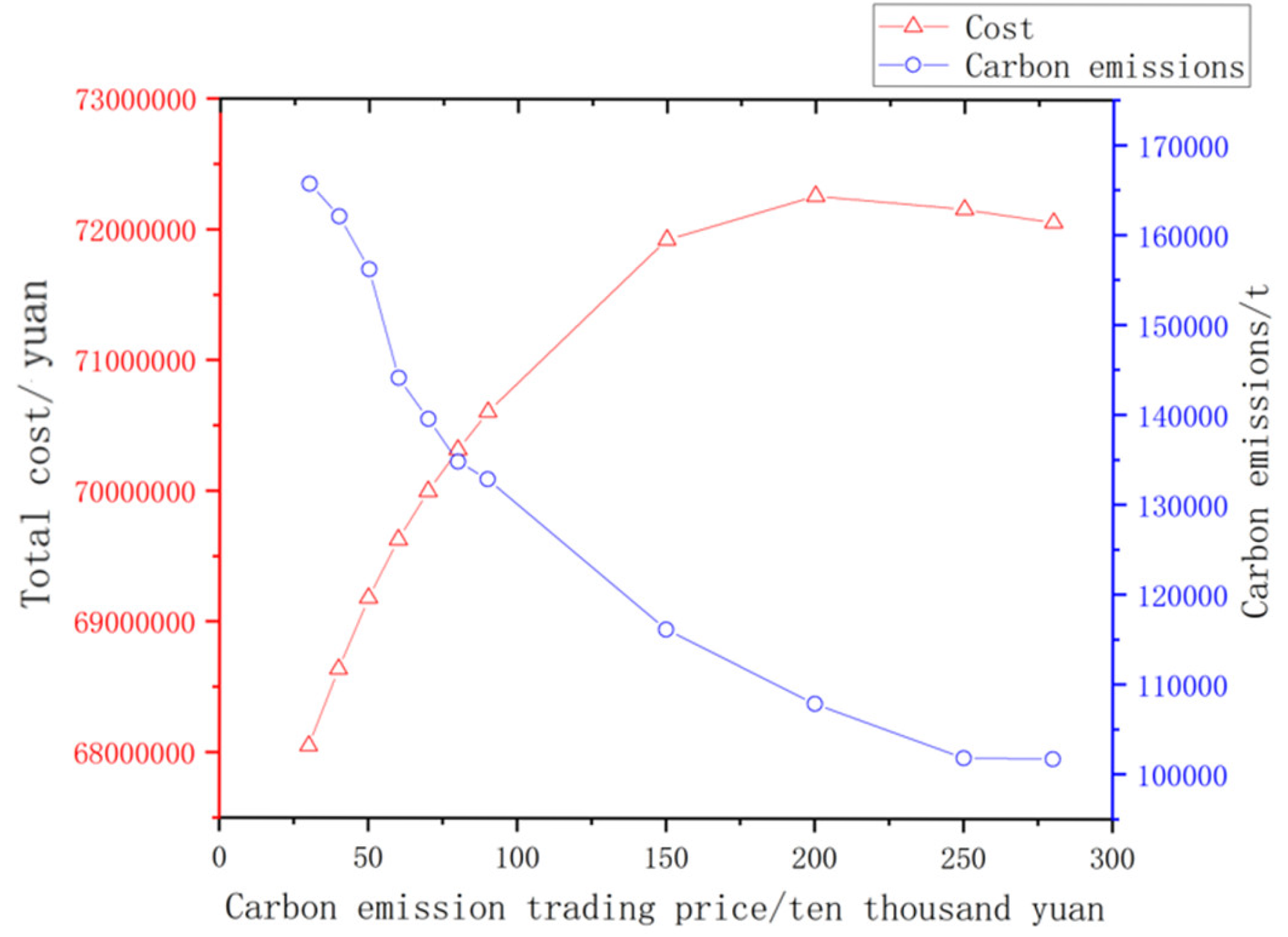
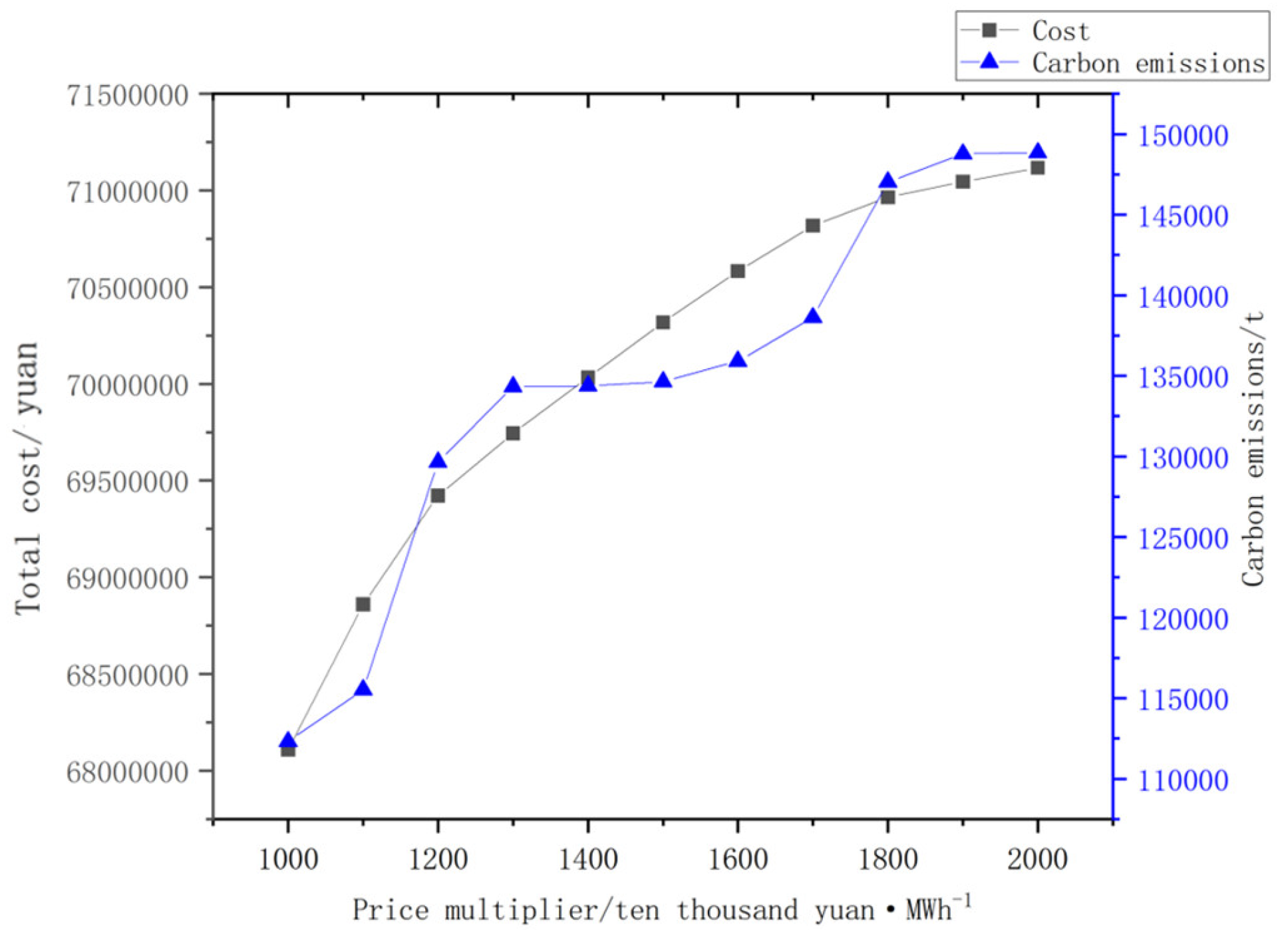
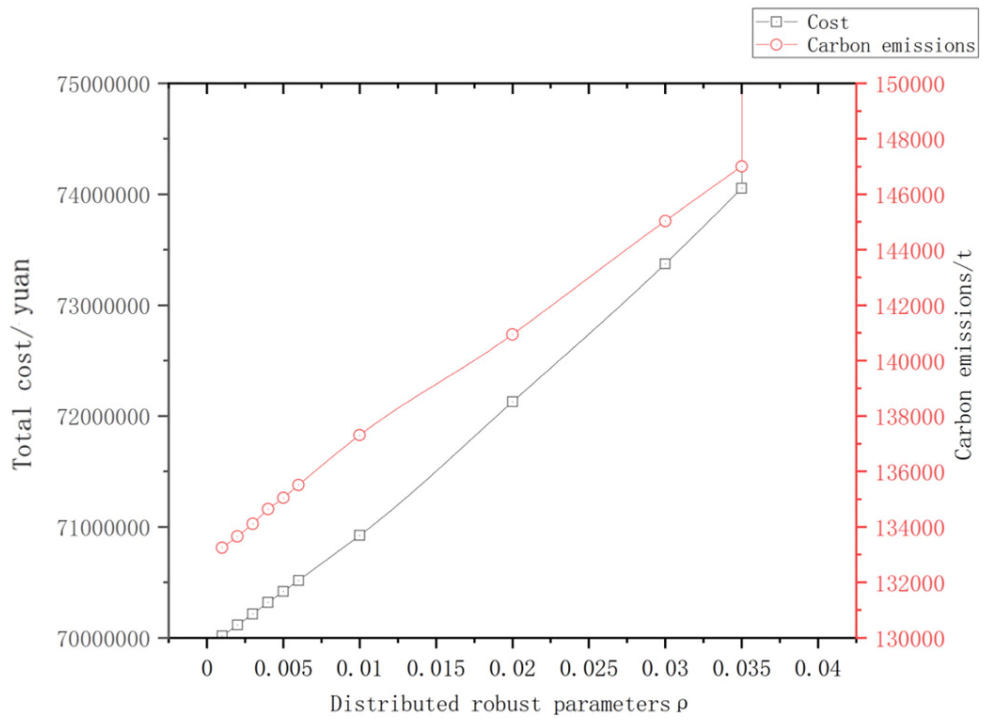
(2)

With the enhancement of carbon trading price, the total operating cost of the system first rises and then falls; the enhancement of load shedding price will lead to an increase in carbon emissions, and when the cost of load shedding is too high, it will no longer be adopted as a way of emission reduction; within a certain range, the distribution robustness parameter d has a small impact on the system cost and carbon emissions, and the reasonable adjustment of this parameter is conducive to the promotion of the system’s economic and low-carbon operation.

The next step of this work will be to conduct an in-depth study of the carbon trading mechanism and consider adding new carbon emission reduction measures to the system to further enhance its emission reduction capability.

References

1. Zhang, H.; Lan, X.; Ye, J.; Huang, H.; Xu, Y.; Ji, A.; Hu, X. The goal and path of source network load storage coordination and interaction to help the construction of a new power system. J. Phys. Conf. Ser. 2023, 2636, 012013. [Google Scholar] [CrossRef]
2. Zhang, X.; Zhao, X.; Zhong, J.; Ma, N. Low carbon multi-objective scheduling of integrated energy system based on ladder light robust optimization. Int. Trans. Electr. Energy Syst. 2020, 30, e12498. [Google Scholar] [CrossRef]
3. Meng, Z.; Dong, F.; Chi, L. Optimal dispatch of integrated energy system with P2G considering carbon trading and demand response. Environ. Sci. Pollut. Res. Int. 2023, 30, 104284–104303. [Google Scholar] [CrossRef] [PubMed]
4. Babahammou, R.H.; Merabet, A.; Miles, A. Technical modelling and simulation of integrating hydrogen from solar energy into a gas turbine power plant to reduce emissions. Int. J. Hydrogen Energy 2024, 59, 343–353. [Google Scholar] [CrossRef]
5. PraveenKumar, S.; Kumar, A. Thermodynamic, environmental and economic analysis of solar photovoltaic panels using aluminium reflectors and latent heat storage units: An experimental investigation using passive cooling approach. J. Energy Storage 2025, 112, 115487. [Google Scholar] [CrossRef]
6. Zhang, J.; Liu, Z. Low carbon economic dispatching model for a virtual power plant connected to carbon capture system considering green certificates-carbon trading mechanism. Sustain. Energy Technol. Assess. 2023, 60, 103575. [Google Scholar] [CrossRef]
7. Su, Z.; Yang, L. Peak shaving strategy for renewable hybrid system driven by solar and radiative cooling integrating carbon capture and sewage treatment. Renew. Energy 2022, 197, 1115–1132. [Google Scholar] [CrossRef]
8. Boré, A.; Dziva, G.; Chu, C.; Huang, Z.; Liu, X.; Qin, S.; Ma, W. Achieving sustainable emissions in China: Techno-economic analysis of post-combustion carbon capture unit retrofitted to WTE plants. J. Environ. Manag. 2023, 349, 119280. [Google Scholar] [CrossRef]
9. Li, M.; Qin, J.; Han, Z.; Niu, Q. Low-carbon economic optimization method for integrated energy systems based on life cycle assessment and carbon capture utilization technologies. Energy Sci. Eng. 2023, 11, 4238–4255. [Google Scholar] [CrossRef]
10. Talaie, M.; Jabari, F.; Foroud, A.A. Modeling and economic dispatch of a novel fresh water, methane and electricity generation system considering green hydrogenation and carbon capture. Energy Convers. Manag. 2024, 302, 118087. [Google Scholar] [CrossRef]
11. Kumar, T.R.; Beiron, J.; Biermann, M.; Harvey, S.; Thunman, H. Plant and system-level performance of combined heat and power plants equipped with different carbon capture technologies. Appl. Energy 2023, 338, 120927. [Google Scholar] [CrossRef]
12. Li, M.; Gao, H.; Abdulla, A.; Shan, R.; Gao, S. Combined effects of carbon pricing and power market reform on CO2 emissions reduction in China’s electricity sector. Energy 2022, 257, 124739. [Google Scholar] [CrossRef]
13. Wang, H.-r.; Feng, T.-T.; Zhong, C. Effectiveness of CO2 cost pass-through to electricity prices under “electricity-carbon” market coupling in China. Energy 2023, 266, 126387. [Google Scholar] [CrossRef]
14. Ma, X.; Pan, Y.; Zhang, M.; Ma, J.; Yang, W. Impact of carbon emission trading and renewable energy development policy on the sustainability of electricity market: A stackelberg game analysis. Energy Econ. 2024, 129, 107199. [Google Scholar] [CrossRef]
15. Ou, Z.; Yang, K.; Lou, Y.; Peng, S.; Li, P.; Zhou, Q. Consider Carbon Emission Flow Analysis of Power System with Regards to Power Loss and Wind Power Uncertainty. J. Phys. Conf. Ser. 2023, 2584, 012107. [Google Scholar] [CrossRef]
16. Wang, G.; Ma, H.; Wang, B.; Alharbi, A.M.; Wang, H.; Ma, F. Multi-Objective Optimal Power Flow Calculation Considering Carbon Emission Intensity. Sustainability 2023, 15, 16953. [Google Scholar] [CrossRef]
17. Chen, S.; Sun, B.; He, Z.; Wu, Z. Calculation method of carbon emission flow in power system based on the theory of power flow calculation. In Proceedings of the 2015 6th International Conference on Manufacturing Science and Engineering, Begawan, Brunei, 1–2 June 2015. [Google Scholar]
18. Huang, J.; Duan, W.; Zhou, Q.; Zeng, H. Methodology for carbon emission flow calculation of integrated energy systems. Energy Rep. 2022, 8, 1090–1097. [Google Scholar] [CrossRef]
19. Wang, C.; Liu, X.; Lee, Y.K. Two-Layer Robust Distributed Predictive Control for Load Frequency Control of a Power System under Wind Power Fluctuation. Energies 2023, 16, 4714. [Google Scholar] [CrossRef]
20. Li, J.; Xiao, Y.; Lu, S. Optimal configuration of multi microgrid electric hydrogen hybrid energy storage capacity based on distributed robustness. J. Energy Storage 2024, 76, 109762. [Google Scholar] [CrossRef]
21. Zhao, X.; Xu, Q.; Yang, Y.; Zhou, G. Distributed distributionally robust optimization of distribution network incorporating novel battery charging and swapping station. Int. J. Electr. Power Energy Syst. 2024, 155 Pt B, 109643. [Google Scholar] [CrossRef]
22. Li, M.; Furifu, C.; Ge, C.; Zheng, Y.; Lin, S.; Liu, R. Distributed Robust Optimal Dispatch for the Microgrid Considering Output Correlation between Wind and Photovoltaic. Energy Eng. 2023, 120, 1775–1801. [Google Scholar] [CrossRef]
23. Wang, J.; Wu, H.; Duan, H.; Zillante, G.; Zuo, J.; Yuan, H. Combining life cycle assessment and Building Information Modelling to account for carbon emission of building demolition waste: A case study. J. Clean. Prod. 2018, 172, 3154–3166. [Google Scholar] [CrossRef]
24. Wang, Y.; Pan, Z.; Zhang, W.; Borhani, T.N.; Li, R.; Zhang, Z. Life cycle assessment f combustion-based electricity generation technologies integrated with carbon capture and storage: A review. Environ. Res. 2022, 207, 112219. [Google Scholar] [CrossRef] [PubMed]
25. Ordoudis, C.; Nguyen, V.A.; Kuhn, D.; Pinson, P. Energy and reserve dispatch with distributionally robust joint chance constraints. Oper. Res. Lett. A J. Oper. Res. Soc. Am. 2021, 49, 291–299. [Google Scholar] [CrossRef]
Figure 2. Comparison chart of wind power forecast.
Energies 18 03522 g002
Figure 3. Comparison chart of photovoltaic prediction.
Energies 18 03522 g003
Figure 4. Optimized system output and load diagram.
Energies 18 03522 g004
Figure 5. Wind and solar uncertainty and energy storage output diagram.
Energies 18 03522 g005
Figure 6. Impact of carbon emission trading price on cost and carbon emissions.
Energies 18 03522 g006
Figure 7. Map of the impact of load-shedding prices on costs and carbon emissions.
Energies 18 03522 g007
Figure 8. The impact of distributed robust parameters on cost and carbon emissions.
Energies 18 03522 g008