Dynamic Identification Method of Distribution Network Weak Links Considering Disaster Emergency Scheduling

Abstract

With the deterioration of the global climate, the losses caused by distribution network failures during natural disasters such as typhoons have become increasingly serious. In the whole process of disaster resistance, it is very important to effectively identify the weak links in distribution networks during typhoon disasters. In this paper, the weak links in distribution networks during typhoons are identified dynamically from four indexes: real-time failure rate, load loss caused by line disconnection, line degree, and line betweenness. First, the Batts typhoon model is established to simulate the whole process of the typhoon and obtain the real-time failure rate of the distribution network. Secondly, the distribution network is powered by distributed generators when there are line disconnections, and a mixed integer linear programming model is established to solve the problem. Then, the line degrees and the line betweenness are calculated to obtain the structure indexes of the line, both of which are dynamically related to the power flow and the loads of the distribution network. Finally, the four indexes are comprehensively analyzed, and the dynamic identification of the weak links in the distribution network are realized by the analytic hierarchy process (AHP)—entropy weight (EW)—technique for order preference by similarity to an ideal solution (TOPSIS) method. The results of the case study show that the proposed method can effectively identify the weak links in a distribution network during a typhoon and provide a reference to resist extreme disasters.

1. Introduction

With the intensification of global climate change, the number of power system accidents caused by extreme disasters has been increasing in recent years. As an important link between power users and the transmission network, the distribution network is a key part of safe and reliable transmission of power. The occurrence of typhoon disasters brings great challenges to the stable operation of distribution networks. The increase of wind speed makes many weak links appear in the distribution network, and these weak links will shift with the change of wind speed caused by the typhoon’s movement. It is very important to adopt appropriate methods to identify the weak links in distribution networks in the process of wind speed change in real time.

The current research on the weak links in distribution networks is mainly divided into three categories: the weak links caused by cyber attacks, the weak links under normal operations and the weak links caused by natural disasters. As for the weak links caused by cyber attacks, [1] proposes a new high-dimensional data-driven cyber-physical attack detection and identification method aimed at the new potential weaknesses introduced by emerging renewable energy, and identifies the risks through the electrical waveform data measured by waveform sensors in the distribution network. The system security of the industrial internet of things has been studied using a machine learning method, and the network vulnerability identified by discussing the industrial internet of things protocol and related vulnerabilities [2]. In [3], a recognition scheme combining dynamic, static and spatial pruning search strategies is proposed to effectively identify critical lines from multiple perspectives in response to malicious attacks on critical lines. As for the weak links in the normal operation of the distribution network, [4] puts forward the concept of the inherent structural characteristics of the power network on the basis of the basic circuit theory, and identifies the weak lines of the system through fast voltage stability index technology based on power flow. In [5], aiming at the operational constraints and uncertainty characteristics of renewable energy power generation, a new schedulable domain method is proposed, which uses the step-to-step search method to process the observation data set and effectively construct the system schedulable domain. In [6], a point estimation method is used to process the overload probability of the line, and the severity function is established to quantify the fluctuation of the line flow. Moreover, the Cholesky method is used to decompose the correlation between simulated load and generation to realize the overload risk assessment of the power line including the wind power system

This paper mainly studies the dynamic identification of the weak links in distribution networks during typhoons. For this research, the effective modeling of the process of a typhoon attacking a power system should first be considered. Based on the storm grade and wind speed, references [7,8] analyze the damage caused by different storm intensities to the power system, and establish the impact assessment model of disasters. Reference [9] analyses the storm events in the database and obtains the influence rule of the storm events by using mathematical statistics. Reference [10] analyses the probabilistic wind model and the assessment of the failure probability of distribution network caused by climate change, and proposes to use a simplified vulnerability curve to represent the impact of extreme disasters on distribution network components. In [11], the topology of a distribution network under extreme weather events is modeled as a Markov state to effectively describe the stochastic process of disasters.

After modeling the disaster process, some studies have identified the weak links in the distribution network under the disaster by various methods. For the study of ice disasters affecting distribution networks, reference [12] combines ice weather events with power system dynamics to propose a numerical simulation method for ice disaster event simulation, which can effectively expand the simulation function of power systems. In [13], by analyzing the relationship between frozen precipitation and wind speed, the Copula function is used to consider the correlation of ice and wind load, and the probability distribution of a line break and tower fall in a distribution network during ice disasters is derived through the connection function. In response to typhoon disasters, reference [14] also considers the weather intensity, fault location, recovery resources, and system scheduling plan when evaluating the resiliency of a transmission system, so as to effectively evaluate the performance of the transmission system during a typhoon. Reference [15] adopts a two-layer programming method to study the vulnerability of power systems, considering both the fault information of the transmission system at the upper level and the emergency operations taken by the grid dispatcher to deal with system faults at the lower level. Similar to reference [4], reference [16], it analyzes the operational domain of power systems during extreme events by using the method of sequential steady-state safety domain. Reference [17], aiming at the characteristics of information–physical interconnection in an active distribution network, takes the shortest path length as the bus vulnerability index, and proposes a bus vulnerability assessment method based on the shortest path function period. Reference [18] also considers the power network interconnection characteristics of the information physical system, and proposes a static analysis method of power system vulnerability based on complex network theory. Reference [19] focuses on the correlation of two-stage failures of distribution network lines, and realizes vulnerability assessments during typhoons based on the multi-scale matrix method. Reference [20] proposes a vulnerable line identification method based on an electrical distance search, which establishes the grid structure by impedance matrix and trims it by connection relation. In [21], the disaster process is regarded as a dual time-dimensional process including weather line break and cascade failure, considering the influence of extreme weather cascading faults. Reference [22] puts forward a method based on current path geometry to realize vulnerable point locations and probability calculations in a power system by constructing a power flow index and a vulnerability index. Reference [23] proposes a vulnerability assessment framework based on the application life of wooden poles, aiming at the impact of the service life of wooden poles on their disaster-bearing capacity, taking into account decay factors and disaster invasion.

For the comprehensive evaluation method, reference [24] proposes a quantitative evaluation framework based on the analytic hierarchy process (AHP) to analyze the effectiveness of the recovery strategy it adopts. Reference [25] evaluates the adaptability of distributed resources to the distribution network through the AHP–entropy weight (EW) method, and verifies the effect of this method through examples. Reference [26] identifies the vulnerable links in the communication network of the power system through the AHP—technique for order preference by similarity to ideal solution (TOPSIS) method. Reference [27] adopts the AHP-EW-TOPSIS method to identify the weak links in a distribution network that is subject to network attacks. The simulation results show that the method can effectively identify vulnerable buses and lines in the distribution network. The comprehensive evaluation method adopted in this paper is applied in the power system and its effectiveness is verified.

As it can be seen from the above, there have been many studies on the identification of weak links in distribution networks during extreme disasters, but most of the existing studies have considered the results of extreme disasters and have not analyzed the dynamic changes in weak links in distribution networks along with the development of disasters during the disaster attack process. The method proposed in this paper is to analyze dynamic changes in weak links in the course of a typhoon according to the pre-disaster typhoon warning. First of all, the Batts model is used to analyze the real-time change in the line failure rate in the distribution network caused by the typhoon, and to establish a line failure model of such a distribution network during typhoons. Then, according to the importance of the location of each line in the distribution network to the transmission of electric energy, the distribution network line degree and line betweenness indexes are calculated. Then, considering the effect of distributed power supply emergency scheduling in the distribution network on the emergency power supply of the isolated island buses during the disaster attack process, the load loss index under the fault of each line of the distribution network is established, the established indexes are comprehensively weighted by AHP-EW-TOPSIS, and the comprehensive index for weak link identification is established. Through the analysis of the results of case studies, the distribution network weak links identification method proposed in this paper can effectively identify the weak links in the distribution network during the typhoon, realize disaster early warning, and enhance the resilience of the distribution network.

2. The Real-Time Failure Rate Index of Distribution Network Lines

In this part, the Batts typhoon model is used to simulate the whole disaster process, obtain the real-time wind speed information of the line, and calculate the real-time failure rate according to the fault characteristics of the line.

2.1. Batts Typhoon Model

In order to effectively simulate the whole effect of a typhoon on the distribution network, the calculation of wind speed at each point of the typhoon is important. This part adopts the Batts typhoon model described in [28].

2.2. Distribution Network Line Fault Model During Typhoon

Faults in distribution network lines during typhoons are mainly caused by the collapse of overhead line poles. The fault model of distribution network pole collapse during a typhoon is mainly calculated through the following equations [29].

2.2.1. Wind Load on Overhead Line Conductors

The model of the wind load on overhead line conductors is

$$w_x=({V_x}^2\alpha {\mu }_s{\mu }_{z}d{l}_x{\sin }^2\theta )/1600$$

(1)

where $w_x$ is the horizontal wind load of the overhead line wire (kN) and $V_x$ is the horizontal wind speed at the overhead line (m/s). Considering that the scale of the typhoon influence range is much larger than the length scale of the distribution network line, unified value processing is adopted for the wind speed on a single line of the distribution network. $\alpha$ is the uneven coefficient of wind pressure, which changes with the change of the wind speed, ${\mu }_s$ is the shape coefficient of the wind load, ${\mu }_z$ is the change coefficient of the wind pressure height, $d$ is the calculated outer diameter of the line (m), $l_x$ is the horizontal span of the line (m), and $\theta$ is the angle between the wind direction and the line.

2.2.2. Wind Load on Overhead Line Poles

The model of the wind load on overhead line poles is

$$w_s={V_s}^2\beta {\mu }_s{\mu }_{z}A/1600$$

(2)

where $w_s$ is the wind load of the distribution pole (kN), $V_s$ is the horizontal wind speed at the overhead line pole (m/s), $\beta$ is the wind vibration coefficient of the line pole, and $A$ is the projected area of the line pole (m²).

2.2.3. Total Load of Overhead Line Poles

The model of the total load is

$$W_s=w_x+w_s$$

(3)

where $W_s$ is the total load of a pole during a typhoon (kN).

2.2.4. Failure Rate of Overhead Line Poles

The failure rate of overhead line poles can be expressed as

$$p(W_s)=\left\{\begin{array}{ccc}{p}_0& & W_s\le W_d\\ {\mathrm{e}}^{[{\displaystyle \frac{\xi (W_s-W_d)}{W_d}}]}-1+p_0& & W_d<W_s\le 2W_d\\ 1& & 2W_d<W_s\end{array}\right.$$

(4)

where $p_0$ is the natural failure probability when the pole is not subjected to a typhoon, $p(W_s)$ is the failure probability of a single overhead line pole, $W_d$ is the design wind load when the pole is manufactured (kN), and $\xi$ is the proportionality coefficient.

2.2.5. Overhead Line Failure Rate

The failure rate of overhead lines is related to the failure rate of poles.

$${\mathcal{P}}_l(V)=1-{\displaystyle \prod _{k=1}^K[1-p_{l,k}(V)]}$$

(5)

where ${\mathcal{P}}_l(V)$ is the failure rate of the line $l$ under typhoon wind speed $V$, $K$ is the total number of poles in the line, and $p_{l,k}(V)$ is the failure rate of pole $k$ in line $l$.

2.2.6. Failure Rate of Overhead Line Based on Monte Carlo Simulation

Monte Carlo simulation mainly determines the probability of event occurrence through random sampling. The failure state of the line can be expressed as

$$F_{l,i}=\left\{\begin{array}{cc}0& Rand\ge {\mathcal{P}}_l\\ 1& Rand<{\mathcal{P}}_l\end{array}\right.$$

(6)

where $F_{l,i}$ denotes the failure state of the line in the first simulation, 1 indicates line failure, and 0 indicates the line has not failed. $Rand$ is the random number generated by the simulation.

$R$ is the number of Monte Carlo samples, and after the simulation, the failure state set of the line is obtained:

$${\Omega }_l=\{F_{l,1},F_{l,2},\dots ,F_{l,R}\}$$

(7)

The line fault probability obtained by Monte Carlo simulation is

$$P_{l,t}^F=n(F_l)/R$$

(8)

where $P_{l,t}^F$ is the line failure probability and $n(F_l)$ is the number of occurrence of line failure under multiple simulations.

3. The Index of Line Degree and Line Betweenness Based on Complex Network Theory

In complex network theory, the line degree and the line betweenness are the key indicators to measure the connectivity of buses and lines in a network. By calculating the line degree and the line betweenness in a distribution network, the importance of lines in the distribution network can be effectively calculated.

3.1. Improved Bus Degrees

The degree index of existing buses mainly considers the number of edges connected to buses [18]. In a distribution network, the location of buses will also affect their importance. Considering the power flow transmission characteristics of the distribution network and its sparsity compared to the transmission network, the inflow power of each bus in the model was set to increase the discrimination. Therefore, the improved degree index of buses is adopted here.

$$D_i^N=P_i{\displaystyle \frac{\sqrt{D_i{\displaystyle \sum _{j\in {\Omega }_i}{D}_j}}}{\overline{D}}}$$

(9)

where $D_i^N$ is the improved bus degree, $D_i$ is the number of lines connected to bus $i$, $\overline{D}$ is the average degree of each bus in the system, ${\Omega }_i$ is the set of adjacent buses, and $P_i$ is the actual incoming power of the bus.

3.2. Line Degrees

Line degrees can be calculated by the formula seen in Equation (10).

$$D_l^L=\sqrt{D_{l1}^N{D}_{l2}^N}$$

(10)

where $D_l^L$ is the degree of the line, and $D_{l1}^N$ and $D_{l2}^N$ are the degrees of improvement in the first and last bus at both ends of the line, respectively.

3.3. Line Betweenness

Line betweenness can be calculated using Equation (11).

$$B_l^L=P_l^L{\displaystyle \sum _{i\in G,j\in N}|\sqrt{P_i{P}_j}{\mathcal{P}}_{ij}(l)|}$$

(11)

where $B_l^L$ is the line betweenness index of the distribution system, $P_l^L$ is the actual transmission active power of the line, $G$ is the set of buses of the distribution network, $N$ is the set of load buses of the distribution network, $P_i$ and $P_j$ are the active power of the corresponding bus, respectively, and ${\mathcal{P}}_{ij}(l)$ is the active power value transmitted by line $l$ when a unit current is separately applied between bus $i$ and bus $j$. The basic model of betweenness can be found in [18].

4. Load Loss Index

After the failure of the distribution network line, the load loss is reduced by island construction and distributed power supply. In this part, the island construction after the fault and distributed power supply optimization are realized by mixed integer linear programming. The load loss after emergency control and optimization is taken as the load loss index caused by a line break.

4.1. Objective Function

The objective function can be expressed as

$$\min L_{l,t}^{Loss}={\displaystyle \sum _{t\in T}{\displaystyle \sum _{i\in N}{\omega }_i(P_{i,t}-P_{i,t}^S})}$$

(12)

where $L_{l,t}^{Loss}$ is the load loss caused by line disconnection at time $t$, $T$ is the number of time periods when the typhoon hits the distribution network, $N$ is the total number of buses in the distribution network, ${\omega }_i$ is the weight of load importance of each bus, $P_{i,t}$ is the load required by the bus, and $P_{i,t}^S$ is the actual power obtained by the bus.

4.2. Constraints

4.2.1. Energy Storage Operation Constraints

These constraints are as follows.

$$0\le P_t^{ch}\le k_t^{ch}{P}^{ch\max }$$

(13)

$$0\le P_t^{dis}\le k_t^{dis}{P}^{dis\max }$$

(14)

$$k_t^{ch}+k_t^{dis}\le 1$$

(15)

$$\left|Q_t^{ES}\right|\le Q_{\max }^{ES}$$

(16)

$$E_{t+1}^{ES}=E_t^{ES}+{\eta }_{ch}{P}_t^{ch}-{\displaystyle \frac{1}{{\eta }_{dis}}}{P}_t^{dis}$$

(17)

$$E_{\min }^{ES}\le E_t^{ES}\le E_{\max }^{ES}$$

(18)

where $P_t^{ch}$ and $P_t^{dis}$, respectively, represent the charging and generating power of the energy storage system; $k_t^{ch}$ and $k_t^{dis}$, respectively, represent the charging and discharging state parameters of the energy storage system; $P^{ch\max }$ and $P^{dis\max }$, respectively, represent the maximum charging and discharging power of the energy storage system; $Q_t^{ES}$ represents the reactive power output of the energy storage system; $Q_{\max }^{ES}$ represents the maximum reactive power output of the energy storage system; $E_t^{ES}$ represents the storage power of the energy storage system; ${\eta }_{ch}$ and ${\eta }_{dis}$, respectively, represent the charging and discharging power factor of the energy storage system; and $E_{\max }^{ES}$ and $E_{\min }^{ES}$ are, respectively, the upper and lower limits of the storage power of the energy storage system.

4.2.2. Gas Turbine Operating Constraints

The constraints are as follows.

$$P^{GT\min }\le P_t^{GT}\le P^{GT\max }$$

(19)

where $P_t^{GT}$ represents the active output of the gas turbine, and $P^{GT\max }$ and $P^{GT\min }$ are the upper and lower limits of the active output of the gas turbine, respectively. In view of the gas turbine output characteristics, only its active output is constrained here.

4.2.3. Bus Power Balance Constraints

Bus power balance constraints encompass both active power balance and reactive power balance.

$$P_{l,t}^{Li}-{\displaystyle \sum _{l\in \Psi \left(i\right)}{P}_{l,t}^L}+P_{i,t}^{GT}+P_{i,t}^{dis}-P_{i,t}^{ch}-P_{i,t}^D=0$$

(20)

$$Q_{l,t}^{Li}-{\displaystyle \sum _{l\in \Psi \left(i\right)}{Q}_{l,t}^L}+Q_{i,t}^{GT}+Q_{i,t}^{ES}-Q_{i,t}^D=0$$

(21)

where $P_{l,t}^{Li}$ and $Q_{l,t}^{Li}$, respectively, represent the incoming active power and reactive power of the superior line of the bus; $\Psi (i)$ represents the line set with the bus as the parent bus; $P_{l,t}^L$ and $Q_{l,t}^L$, respectively, represent the active power and reactive power transmitted by the line; $P_{i,t}^{GT}$ and $Q_{i,t}^{GT}$, respectively, represent the active power and reactive power of the gas turbine at the bus; $P_{i,t}^{ch}$ and $P_{i,t}^{dis}$, respectively, represent the energy storage charging and discharging power at bus $i$; $Q_{i,t}^{ES}$ is the reactive power output of the energy storage device at bus $i$; and $P_{i,t}^D$ and $Q_{i,t}^D$ are, respectively, the active power and reactive power load of bus $i$.

4.2.4. Power Flow Equality Constraints

The Distflow model [30] is used to represent the power flow equality constraints of the distribution network.

$$U_{i,t}-U_{j,t}\le \left(1-X_{l,t}\right)M+2\left(r_l{P}_{l,t}^L+x_l{Q}_{l,t}^L\right)$$

(22)

$$U_{i,t}-U_{j,t}\le \left(X_{l,t}-1\right)M+2\left(r_l{P}_{l,t}^L+x_l{Q}_{l,t}^L\right)$$

(23)

where $U_{i,t}$ represents the voltage squared of bus $i$, and $X_{l,t}$ represents the line state (normal operation is 1, broken line is 0). Here, $M$ is used to relax this constraint into a linearization constraint. $r_l$ and $x_l$ are, respectively, the resistance and reactance of the line.

4.2.5. Voltage Constraints

The bus voltage needs to be maintained within the range required for power grid operation.

$$V_{i\min }^2\le U_{i,t}\le V_{i\max }^2$$

(24)

where $V_{i\max }$ and $V_{i\min }$ are, respectively, the upper and lower limits of the bus voltage.

4.2.6. Line Capacity Constraints

The constraints are as follows.

$${\left(P_{l,t}^L\right)}^2+{\left(Q_{l,t}^L\right)}^2\le X_{l,t}{S}_l$$

(25)

where $S_l$ represents the maximum transmission capacity of the line. In the operation of the distribution network, the line power flow needs to meet the above capacity constraints, but the above constraints are nonlinear constraints, which cannot be solved directly by the solver, and are converted into linear constraints by the following formulas.

$$-X_{l,t}{S}_l\le P_{l,t}^L\le X_{l,t}{S}_l$$

(26)

$$-X_{l,t}{S}_l\le Q_{l,t}^L\le X_{l,t}{S}_l$$

(27)

$$-\sqrt{2}{X}_{l,t}{S}_l\le P_{l,t}^L+Q_{l,t}^L\le \sqrt{2}{X}_{l,t}{S}_l$$

(28)

$$-\sqrt{2}{X}_{l,t}{S}_l\le P_{l,t}^L-Q_{l,t}^L\le \sqrt{2}{X}_{l,t}{S}_l$$

(29)

5. Distribution Network Weak Link Identification Comprehensive Index

5.1. Aggregative Index

After the construction of the aforementioned sub-indicators, a comprehensive indicator for identifying weak links is obtained.

$${\mathfrak{W}}_{L,t}={\lambda }_1{P}_{l,t}^F+{\lambda }_2{L}_{l,t}^{Loss}+{\lambda }_3{D}_{l,t}^L+{\lambda }_4{B}_{l,t}^L$$

(30)

where ${\mathfrak{W}}_{l,t}$ is the weakness index of the line $l$ at the time period $t$, $P_{l,t}^F$ is the failure rate index, $L_{l,t}^{Loss}$ is the load loss index, $D_{l,t}^L$ is the line degree index, $B_{l,t}^L$ is the line betweenness index, and ${\lambda }_1~{\lambda }_4$ are the weights of each sub-index. The proposed distribution network line weakness index takes into account the line failure rate, the load loss caused by line failure, line degree, and line betweenness.

Since all indicators in the weak link identification are positive indicators, the following formula is used to normalize the data of each indicator.

$$x^{std}={\displaystyle \frac{x-x_{\min }}{x_{\max }-x_{\min }}}$$

(31)

where $x^{std}$ represents the normal value of each index after normalization, $x$ is the original value of each indicator, and $x_{\max }$ and $x_{\min }$ are the maximum and minimum value of the evaluation index, respectively.

The normalized matrix $X^{std}$ is as follows:

$$X^{std}=\left[\begin{array}{cccc}{x}_{11}^{std}& x_{12}^{std}& x_{13}^{std}& x_{14}^{std}\\ x_{21}^{std}& x_{22}^{std}& x_{23}^{std}& x_{24}^{std}\\ ⋮& ⋮& ⋮& ⋮\\ x_{m1}^{std}& x_{m2}^{std}& x_{m3}^{std}& x_{m4}^{std}\end{array}\right]$$

(32)

The index evaluation system was constructed through AHP, EW, and TOPSIS.

5.2. Analytic Hierarchy Process

The analytic hierarchy process [25] is a subjective evaluation method in the evaluation of indicators. The importance of indicators is assigned by subjective factors, the comparison matrix is constructed, and the weight of each index is obtained by consistency test.

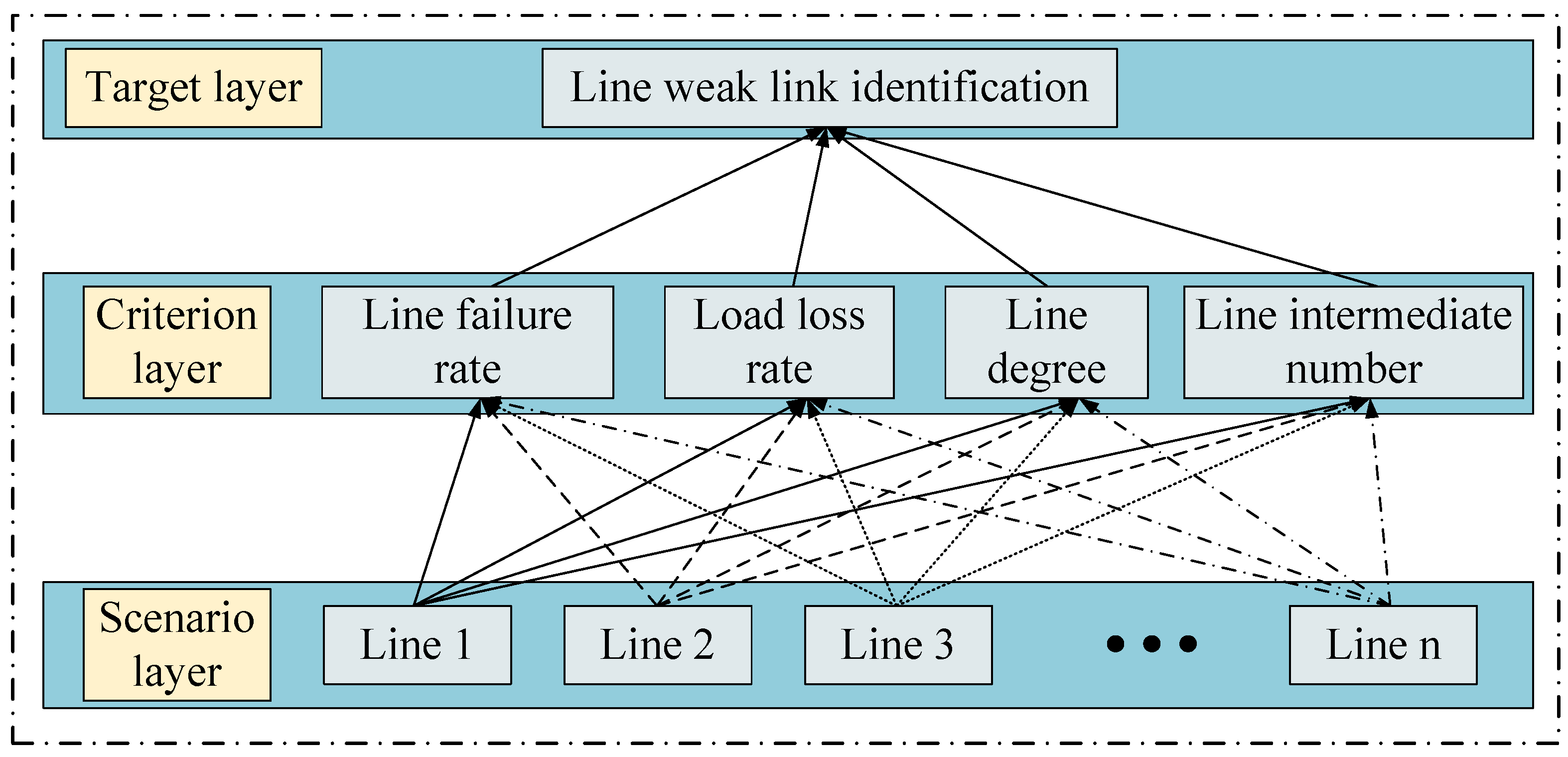
5.2.1. Establishing the Hierarchical Structure Model

In order to locate the weak link in the criterion layer, the probability of line failure, load loss rate caused by line failure, line degree, and line betweenness are considered. Each line failure is taken into account in the analysis scheme, and the hierarchical model is shown in the following Figure 1:

5.2.2. Comparison Matrix Construction

The matrix is

$$\mathcal{C}=\left[\begin{array}{cccc}{C}_{11}& C_{12}& C_{13}& C_{14}\\ C_{21}& C_{22}& C_{23}& C_{24}\\ C_{31}& C_{32}& C_{33}& C_{34}\\ C_{41}& C_{42}& C_{43}& C_{44}\end{array}\right]$$

(33)

where $\mathcal{C}$ is the importance comparison matrix of each indicator and $C_{ij}(i\ne j)$ is the ratio of the importance parameters between the indicator $i$ and the indicator $j$, which is mainly determined by the following

Table 1. The importance of each index is compared.

Comparative Scale	Significance	Comparative Scale	Significance
1	Pairwise comparisons are equally important	7	Pairwise is more important than the former
3	Pairwise is slightly more important than the former	9	Pairwise is more important than the former
5	Pairwise is obviously more important than the former	$2m (m=1,2,3,4)$	The importance is somewhere in the middle

:

The comparison matrix of the four indicators in this part is

$$\mathcal{C}=\left[\begin{array}{cccc}1& 2& 5& 4\\ {\displaystyle \frac{1}{2}}& 1& 4& 3\\ {\displaystyle \frac{1}{5}}& {\displaystyle \frac{1}{4}}& 1& 2\\ {\displaystyle \frac{1}{4}}& {\displaystyle \frac{1}{3}}& {\displaystyle \frac{1}{2}}& 1\end{array}\right]$$

(34)

The matrix shows that the probability of line failure and the load loss rate caused by line failure occupy a higher proportion in the network weakness index than the number of line degrees and the line betweenness, which accords with the judgment logic of the weak link in the actual situation. The sequence of each indicator corresponds to (30).

5.2.3. Weight Matrix Calculation and Consistency Check

The consistency index can be calculated using Equation (35).

$$CI={\displaystyle \frac{{\lambda }_{\max }-N}{N-1}}$$

(35)

where $CI$ is the consistency index, ${\lambda }_{\max }$ is the largest characteristic root of the matrix, and $N$ is the order of the matrix.

$$CR={\displaystyle \frac{CI}{RI}}$$

(36)

where $CR$ is the index test value and $RI$ is the corresponding average random consistency index, values of which are shown in the following

Table 2. Average random consistency index.

N	1	2	3	4	5	6	7	8	…
RI	0	0	0.52	0.89	1.12	1.26	1.36	1.41

.

By calculation, CI = 0.0463; the maximum characteristic root is 4.1389; index test value CR = 0.0520 < 1 meets the requirements; and the weights $\omega$ of the four indexes are 0.4900, 0.3075, 0.1128, and 0.0897, respectively.

5.3. Entropy Weight Method

The entropy weight method [25] is a relatively objective evaluation method among index evaluation methods, which only relies on the discreteness of the data itself, and does not deal with it by subjective assignment.

5.3.1. Index Proportion Calculation

The calculation formula is

$${\eta }_{ij}={\displaystyle \frac{x_{ij}^{std}}{{\displaystyle \sum _{i=1}^m{x}_{ij}^{std}}}}$$

(37)

where $m$ is the number of samples and ${\eta }_{ij}$ is the proportion of the index $j$ of sample $i$.

5.3.2. Entropy Index Value Calculation

The calculation formula is

$$e_j=-{\displaystyle \frac{1}{\ln m}}{\displaystyle \sum _{i=1}^m{\eta }_{ij}\ln {\eta }_{ij}}$$

(38)

where $e_j$ represents the entropy index value of the $j$th index.

5.3.3. Entropy Weight Calculation

The calculation formula is

$${\mu }_j={\displaystyle \frac{1-e_j}{m-{\displaystyle \sum _{i=1}^m{e}_j}}}$$

(39)

where ${\mu }_j$ represents the entropy weight of the $j$th index.

5.3.4. Subjective and Objective Comprehensive Weight Calculation

The calculation formula is

$${\lambda }_j={\displaystyle \frac{\sqrt{{\mu }_j{\omega }_j}}{{\displaystyle \sum _{j=1}^n\sqrt{{\mu }_j{\omega }_j}}}}$$

(40)

where ${\lambda }_j$ represents the subjective and objective comprehensive weights of indicator $j$.

5.4. TOPSIS Method Comprehensive Weight Analysis

5.4.1. Original Matrix Standardization

The TOPSIS method [27] first requires the processing of data.

$$Z^{TOP}=\left[\begin{array}{cccc}{z}_{11}& z_{12}& \dots & z_{1n}\\ z_{21}& z_{22}& \dots & z_{2n}\\ ⋮& ⋮& \ddots & ⋮\\ z_{m1}& z_{m2}& \dots & z_{mn}\end{array}\right]=\left[\begin{array}{cccc}{\displaystyle \frac{x_{11}}{\sqrt{{\displaystyle {\sum }_{i=1}^m{x}_{i1}^2}}}}& {\displaystyle \frac{x_{12}}{\sqrt{{\displaystyle {\sum }_{i=1}^m{x}_{i2}^2}}}}& \dots & {\displaystyle \frac{x_{1n}}{\sqrt{{\displaystyle {\sum }_{i=1}^m{x}_{in}^2}}}}\\ {\displaystyle \frac{x_{21}}{\sqrt{{\displaystyle {\sum }_{i=1}^m{x}_{i1}^2}}}}& {\displaystyle \frac{x_{22}}{\sqrt{{\displaystyle {\sum }_{i=1}^m{x}_{i2}^2}}}}& \dots & {\displaystyle \frac{x_{2n}}{\sqrt{{\displaystyle {\sum }_{i=1}^m{x}_{in}^2}}}}\\ ⋮& ⋮& \ddots & ⋮\\ {\displaystyle \frac{x_{m1}}{\sqrt{{\displaystyle {\sum }_{i=1}^m{x}_{i1}^2}}}}& {\displaystyle \frac{x_{m2}}{\sqrt{{\displaystyle {\sum }_{i=1}^m{x}_{i2}^2}}}}& \dots & {\displaystyle \frac{x_{mn}}{\sqrt{{\displaystyle {\sum }_{i=1}^m{x}_{in}^2}}}}\end{array}\right]$$

(41)

where $z$ is the standardized value and $Z^{TOP}$ is the standardized matrix.

5.4.2. Weighted Index Evaluation Matrix Calculation

The calculation formula is

$$\mathcal{V}=\left[\begin{array}{cccc}{v}_{11}& v_{12}& \dots & v_{1n}\\ v_{21}& v_{22}& \dots & v_{2n}\\ ⋮& ⋮& \ddots & ⋮\\ v_{m1}& v_{m2}& \dots & v_{mn}\end{array}\right]=\left[\begin{array}{cccc}{\lambda }_1{z}_{11}& {\lambda }_2{z}_{12}& \dots & {\lambda }_n{z}_{1n}\\ {\lambda }_1{z}_{21}& {\lambda }_2{z}_{22}& \dots & {\lambda }_n{z}_{2n}\\ ⋮& ⋮& \ddots & ⋮\\ {\lambda }_1{z}_{m1}& {\lambda }_2{z}_{m2}& \dots & {\lambda }_n{z}_{mn}\end{array}\right]$$

(42)

where $v$ is the weighted index value and $\mathcal{V}$ is the weighted index evaluation matrix.

Positive ideal value:

$${\mathcal{V}}^{+}=(v_1^{+},v_2^{+},v_3^{+},\dots ,v_n^{+})=\left\{\max v_{ij}|i=1,2,3,\dots ,m\right\}$$

(43)

where $v^{+}$ is the positive ideal value and ${\mathcal{V}}^{+}$ is the positive ideal value group.

Negative ideal value:

$${\mathcal{V}}^{-}=(v_1^{-},v_2^{-},v_3^{-},\dots ,v_n^{-})=\left\{\min v_{ij}|i=1,2,3,\dots ,m\right\}$$

(44)

where $v^{-}$ is the negative ideal value and ${\mathcal{V}}^{-}$ is the group of negative ideal values.

Distance from single index to ideal value:

$$D_i^{+}=\sqrt{{\displaystyle \sum _{j=1}^n{(v_j^{+}-v_{ij})}^2}}$$

(45)

$$D_i^{-}=\sqrt{{\displaystyle \sum _{j=1}^n{(v_j^{-}-v_{ij})}^2}}$$

(46)

where $D_i^{+}$ and $D_i^{-}$ are the positive distance and negative distance of each index to the ideal value, respectively

Relative fit of each index value:

$$S_i={\displaystyle \frac{D_i^{-}}{(D_i^{+}+D_i^{-})}}$$

(47)

The index of the identified object is sorted by the relative fit degree $S_i$ of each index value.

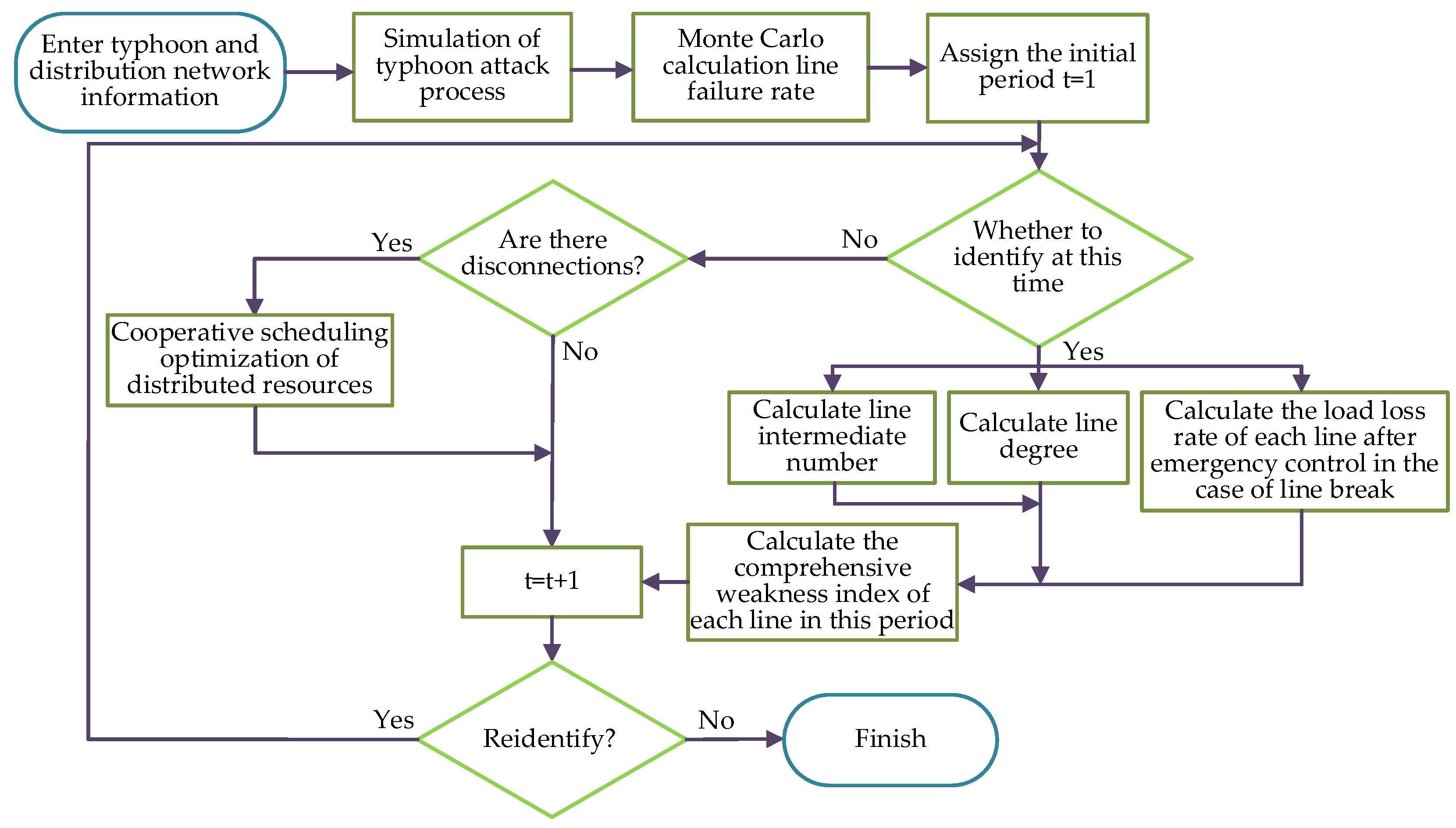
5.5. Solving Process of Identification Model

The model proposed mainly includes the simulation of a typhoon and the calculation of various weak indexes under emergency control. The main solving steps of the model are shown in the following Figure 2:

6. Case Study

In this part, the proposed model is verified and analyzed by taking the IEEE 33-bus system [31] as an example. The enhanced system topology is shown in Figure 3. The numbers in the middle of the lines are the line serial numbers, the numbers beside the buses are the bus serial numbers, the dashed circles indicate the range of the typhoon.

6.1. Introduction of the Case

In the enhanced IEEE 33-bus system, gas turbine equipment is configured on bus 8 and 28, their maximum active power output being 0.3 MW and 0.25 MW, respectively. The energy storage equipment is configured on bus 15, its maximum discharge power being 0.2 MW and its maximum discharge capacity being 0.8 MWh. The period from 22:00 to 4:00 the next day is taken as the typhoon impacting the distribution network, divided into 24 periods of 15 min each. Load data refers to [31]. In terms of load, buses 3, 4, and 10 are first-level loads, with weights of 100; buses 8, 14, 25, and 30 are second-level loads, with weights of 10; and the rest of the loads are third-level loads, weighted 1. The angle between the typhoon moving direction and the horizontal axis is 30°. The initial pressure of the typhoon center is 975 hpa and the typhoon is moving at 35 km/h. The model parameters of overhead line poles all refer to normative documents. The model proposed in this paper was simulated and solved using Matlab R2022b.

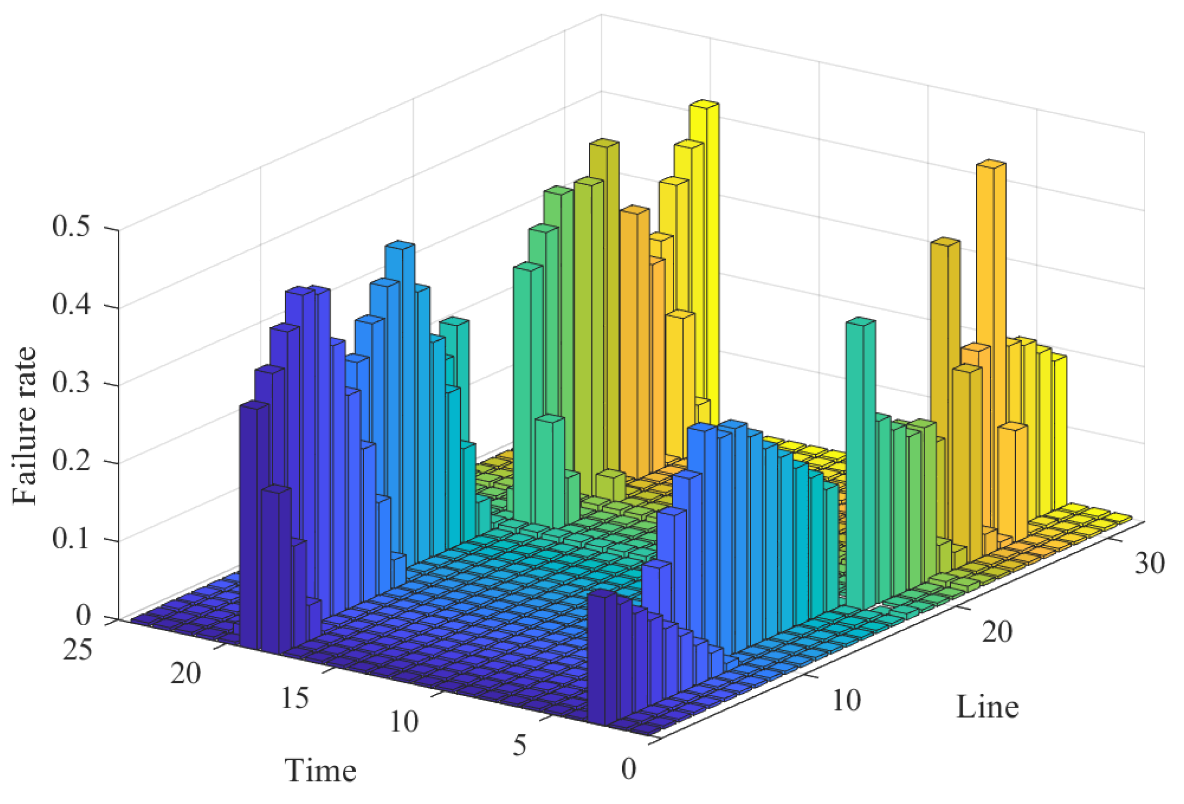
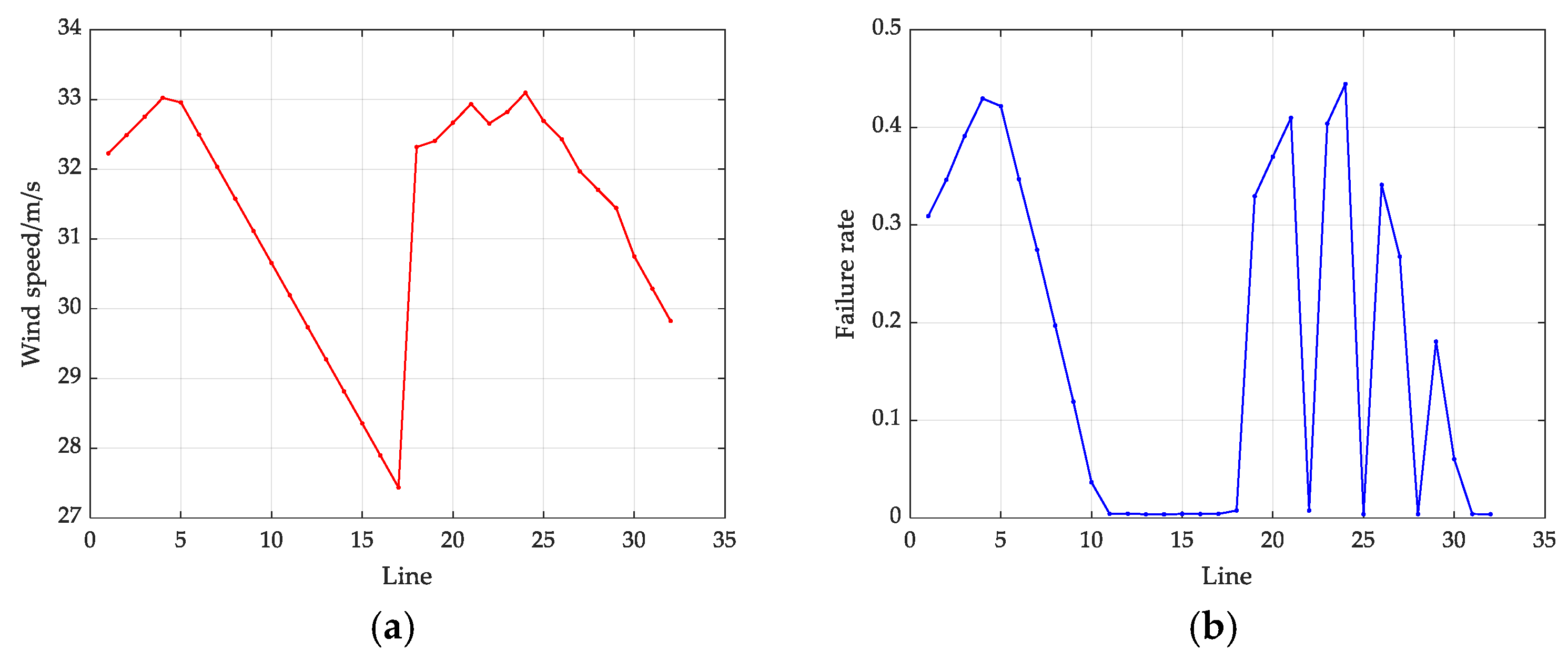
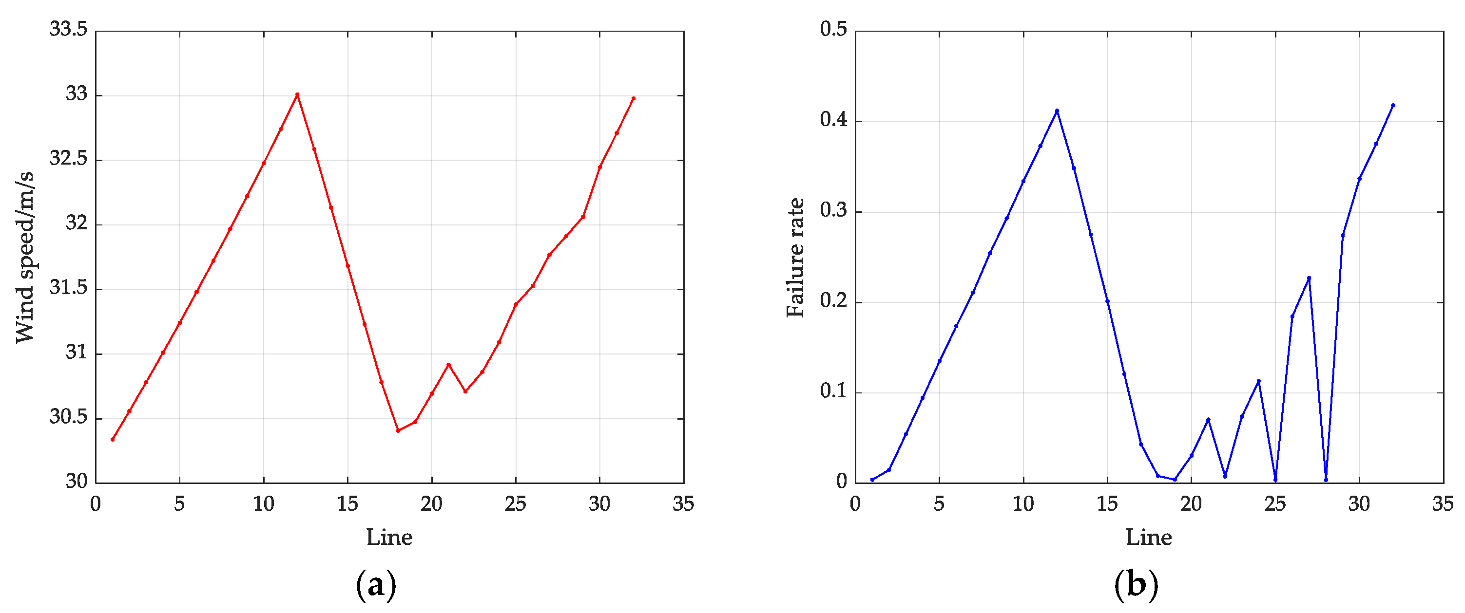
6.2. Real-Time Failure Rate Change Diagram of Each Line

When a typhoon strikes the distribution network, the position of the typhoon changes with time, which leads to the real-time change of the line failure rate. The change curve of the line failure rate of the distribution network is shown in Figure 4. The different color bars in the figure represent the failure rates of different lines.

As can be seen from the figure, there are two peaks in the failure rate of some lines in the distribution network, mainly because during the typhoon, some lines appear twice at the maximum wind speed radius of the typhoon, which is consistent with the actual situation.

6.3. Identification and Analysis of Weak Links in Distribution Network During Existing Line Failures

In the above model, which combines subjective and objective comprehensive identification indicators, the comprehensive weights $\lambda$ of the four indicators are 0.3704, 0.2934, 0.1777, and 0.1584, respectively.

6.3.1. Analysis of Identification Results of Line Weak Links

In this part, the case of line 6 breaks in time period 4 is case 1. Considering the change characteristics of the line failure rate, the difference between the failure rates of various lines in some time periods is lower, so the identification results of the weak links in time period 18 in this case are taken for analysis. The identification ranking and total index values are shown in

Table 3. Identification results in case 1.

Rank	Line	Index Value	Rank	Line	Index Value
1	1	0.1975	17	24	0.0195
2	2	0.1611	18	29	0.0182
3	19	0.0922	19	30	0.0113
4	3	0.0814	20	14	0.0086
5	20	0.0451	21	31	0.0074
6	22	0.0387	22	10	0.0058
7	23	0.0372	23	12	0.0055
8	4	0.0346	24	13	0.0054
9	5	0.0315	25	11	0.0053
10	25	0.0285	26	32	0.0040
11	26	0.0254	27	21	0.0039
12	8	0.0253	28	16	0.0037
13	9	0.0250	29	17	0.0037
14	18	0.0235	30	7	0.0036
15	27	0.0229	31	15	0.0035
16	28	0.0209	32	6	0

.

As can be seen from Table 3, in case 1, the top five lines in terms of vulnerability are line 1, 2, 19, 3, and 20, respectively. Among the comprehensive vulnerability indicators, the failure rate has the greatest weight, and the failure rate curve of each line in the 18th period is shown in Figure 5.

As can be seen from the figure, in the 18th period, the failure rates of lines 1, 19, 2, 20, and 3 are significantly higher than those of other lines, so their weak indexes will also increase to a certain extent. In Table 3, the index rankings of these lines are all within the top ten.

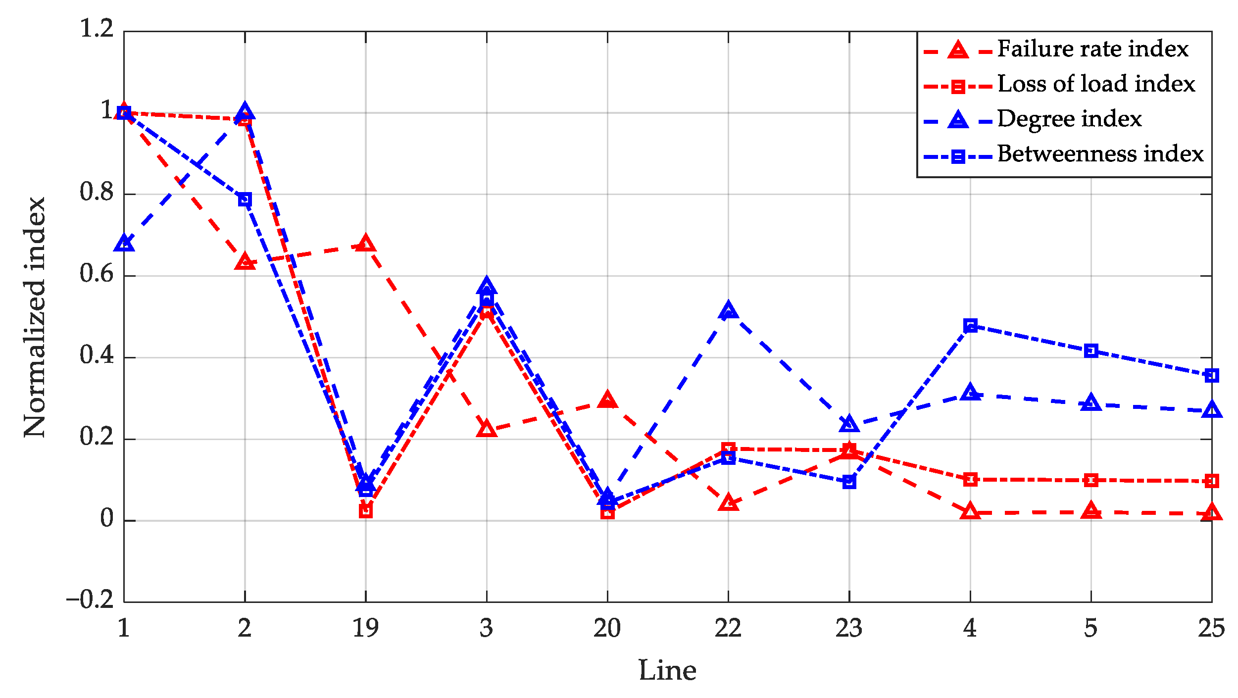
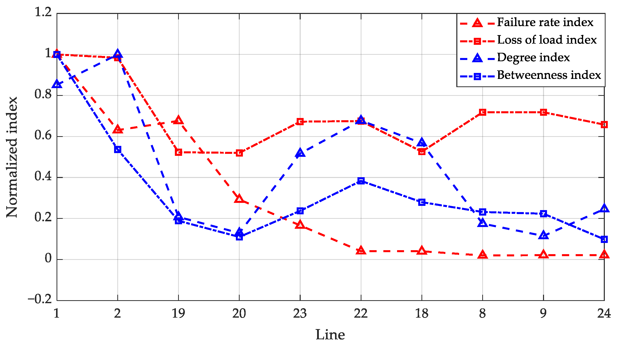
6.3.2. Analysis of Each Index of Line Weakness

The top ten lines of the line weakness identification results in case 1 were selected for analysis, and their sub-index values are shown in Figure 6 below.

It can be seen from the curve in the figure that the factors determining the total index value of each line correspond to each index value. For lines 19 and 20, their top ranking mainly depends on their high failure rate index value. Because of the important position of line 1 and 2 in the network structure, the load loss index, degree index, and interface index are higher, so even in the case of a similar failure rate index, the ranking is higher. Although the failure rate index of line 3 is relatively low, the other three indicators are relatively high, so the ranking is higher than that of line 20. It can be seen that the influence degree of each sub-index value on the total index is closely related to its index weight. The weak link identification method proposed in this paper can effectively identify the weak links caused by the typhoon.

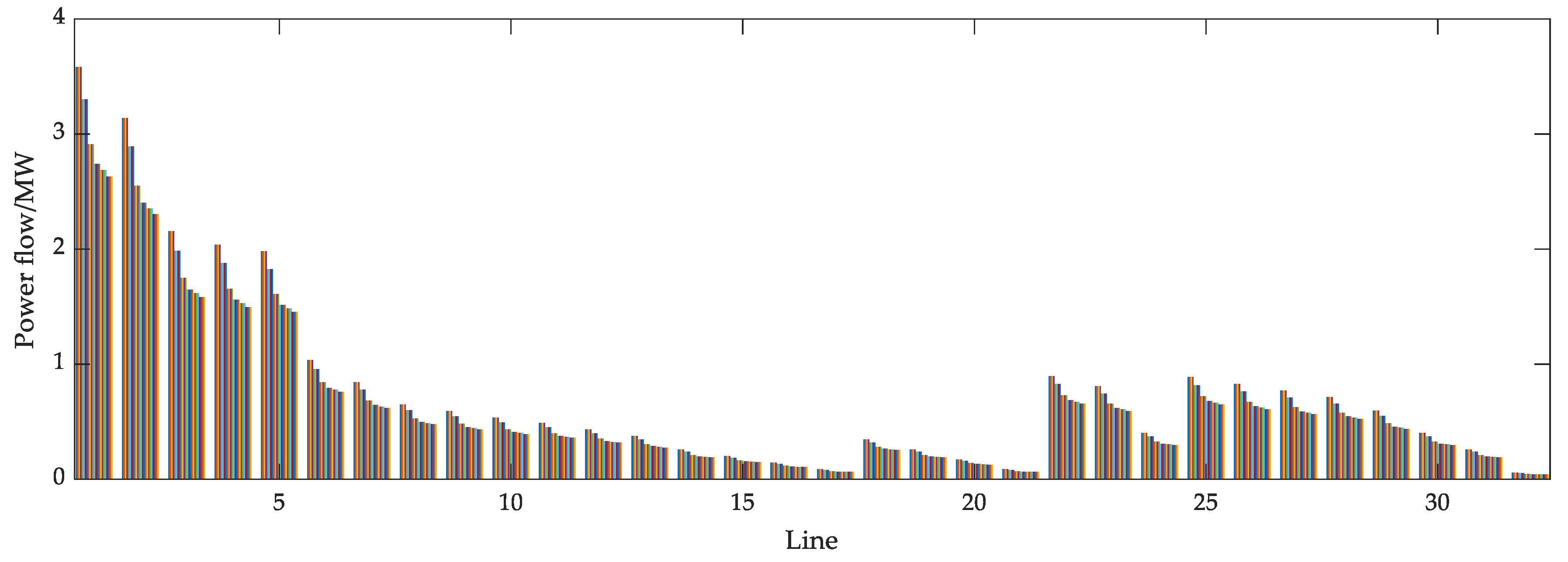
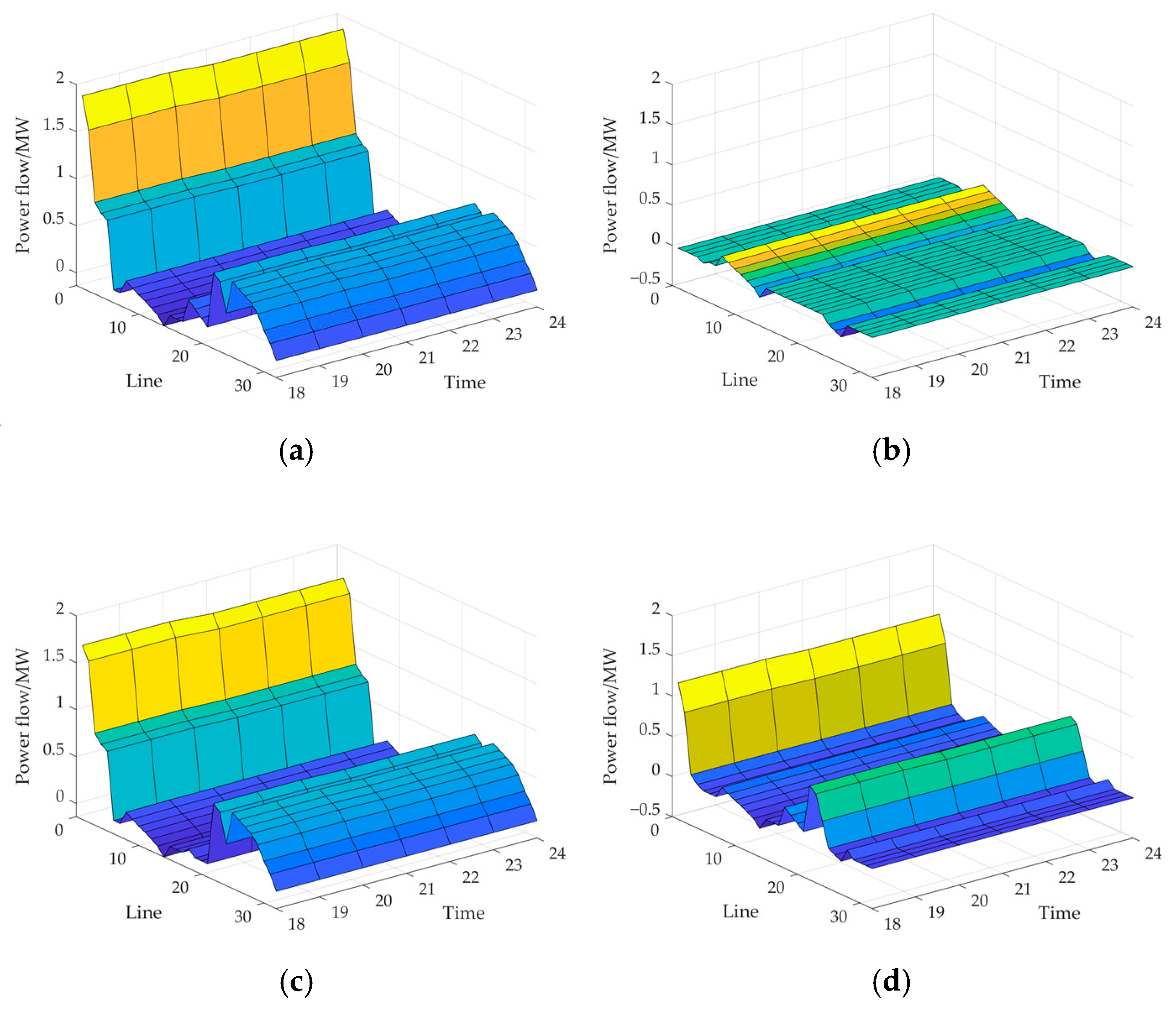
6.3.3. Power Flow Change of Each Line During the Identification Period

The initial power flow distribution of the system without fault is shown in Figure 7. The different color bars in Figure 7 represent the power flow in different time periods. In order to compare the influence of different line breaks on the system power flow change under the identification results in this paper, line 1, line 19, and line 5 among the top 10 weak lines under the identification results of case 1 were selected for comparison. Since the identification period is the 18th period, the remaining line disconnection before the 18th period is not considered, so the comparison period is the 18–24th period. The results are shown as Figure 8. The different colors in Figure 8 represent the power flow of different lines.

As can be seen, for the case in Figure 8a where there is no line break in the 18th period, the system power flow distribution shows a decreasing rule with the structure diffusion. Lines 7–17 lose the power supply of the upper circuit due to the line break, so the line active power transmission is especially small. Although bus 15 has distributed resources, however, distributed resources can only supply power to some buses in some periods, so the transiting power of this part is low. In Figure 8b, the change of power flow output varies greatly compared with the situation without fault, mainly because line 1 is at a key position in the distribution network system, so all buses lose their power supply of the upper circuit due to line 1 disconnection, and only the power flow generated by the distributed resource power supply is present, while line 1 also has a high failure rate, so it is the weakest line during this period. The failure of line 19 and line 5 can only affect the power supply of a few buses, so the difference between the power flow change and the no-fault condition is smaller, and the load loss index is also smaller than line 1. The power flow change of the two lines occurs mainly because the upper line reduces the power supply to the island buses.

6.3.4. The Output Change of Each Distributed Resource After the Identification Period

In order to reflect the dynamic characteristics of coordinated control of distributed resources considered in this paper, the output of distributed resources under the disconnection of each identification line is analyzed. In case 1, there are no distributed resources that can be called in the subordinate lines of line 19, so the disconnection cases of line 9 are selected for comparison. The results are shown in Figure 9.

As can be seen from Figure 9, distributed resources dynamically adjust the active power output strategy according to the power supply path of the system for different line disconnections. In the case of only line 6 breaking, the gas turbine of bus 28 will not output electrical energy. In the case of line 9 breaking, as per Figure 9a, only ESS1 and GT1 output electrical energy, due to the influence of the line break, the island power supply ranges of the two sources are changed, and the outputs of ESS1 and GT1 are also different. In the case of line 1 and line 5 disconnection, all three distributed resources will output power. Due to the large island power supply range of GT2 in both cases, GT2 is in high power operation when line 1 and line 5 are disconnected, and there is no difference between them. The results of the example effectively demonstrate the dynamic coordination characteristics of distributed resources to improve the resilience of power grids.

6.4. Comparison of Identification Results of Weak Links Under Different Failure Conditions

The identification results of the distribution network weak link in case 1 have been analyzed above. In order to reflect the real-time characteristics of the method proposed in this paper, the identification results of different fault situations in the distribution network at the same time are compared. In case 2, line 6 breaks in the 4th period and line 3 breaks in the 15th period. The identification results of the weak links in the 18th period in this case are shown in

Table 4. The identification results in the 18th period in case 2.

Rank	Line	Index Value	Rank	Line	Index Value
1	1	0.1435	17	26	0.0215
2	2	0.1006	18	25	0.0208
3	19	0.0821	19	21	0.0206
4	20	0.0425	20	5	0.0204
5	23	0.0425	21	16	0.0202
6	22	0.0419	22	17	0.0202
7	18	0.0348	23	30	0.0202
8	8	0.0304	24	7	0.0201
9	9	0.0297	25	29	0.0201
10	24	0.0279	26	28	0.0201
11	14	0.0245	27	32	0.0201
12	10	0.0233	28	4	0.0201
13	11	0.0230	29	15	0.0201
14	13	0.0229	30	31	0.0201
15	12	0.0229	31	3	0
16	27	0.0225	32	6	0

.

As can be seen from the above table, the identification results of weak links in the distribution network in the 18th period in case 2 are not much different from those in case 1: some lines still have a higher ranking due to the higher line failure rate, and the disconnection of line 3 mainly affects the line degree and power transmission of its neighboring lines, and also affects the importance of power transmission of its superior lines, so the positions of line 4 and line 5 are switched. For line 6 and line 3, due to the breaking reason, the weakest degree is treated in the identification of the weak links in the 18th period.

In case 2, the sub-index values of the identification results for the 18th period are shown in Figure 10.

It can be seen from Figure 10 that line 3 breakage has an impact on the sub-index value of each line, resulting in the mutual cancellation of the influence on the overall ranking of line weakness, and the change in the ranking of line weakness is small.

6.5. Comparison of Identification Results of Weak Links in Different Identification Periods

Since the model proposed in this paper is the real-time identification of weak links in the distribution network, it is necessary to compare the changes of the weak links in different time periods of the distribution network. The identification results of different time periods in case 1 are taken as an example to illustrate. The identification results of time periods 19 and 20 are shown in

Table 5. Identification results in the 19th period in case 1.

Rank	Line	Index Value	Rank	Line	Index Value
1	2	0.1203	17	9	0.0267
2	1	0.1127	18	25	0.0238
3	3	0.0815	19	18	0.0186
4	4	0.0559	20	28	0.0173
5	5	0.0542	21	30	0.0123
6	24	0.0517	22	14	0.0067
7	23	0.0514	23	10	0.0065
8	26	0.0461	24	31	0.0057
9	21	0.0445	25	13	0.0038
10	20	0.0419	26	11	0.0037
11	19	0.0390	27	12	0.0036
12	27	0.0388	28	32	0.0022
13	8	0.0337	29	17	0.0015
14	7	0.0327	30	15	0.0015
15	22	0.0320	31	16	0.0015
16	29	0.0284	32	6	0

and

Table 6. Identification results in the 20th period in case 1.

Rank	Line	Index Value	Rank	Line	Index Value
1	2	0.0810	17	5	0.0303
2	1	0.0791	18	4	0.0297
3	3	0.0561	19	22	0.0290
4	32	0.0441	20	7	0.0261
5	12	0.0439	21	15	0.0251
6	31	0.0419	22	23	0.0221
7	11	0.0411	23	25	0.0216
8	9	0.0407	24	24	0.0215
9	30	0.0396	25	18	0.0169
10	13	0.0393	26	16	0.0160
11	10	0.0382	27	28	0.0157
12	8	0.0376	28	21	0.0099
13	29	0.0367	29	17	0.0061
14	27	0.0341	30	19	0.0059
15	14	0.0338	31	20	0.0058
16	26	0.0312	32	6	0

, the value of each component index is shown in Figure 11 and Figure 12, and the line failure rate curve is shown in Figure 13 and Figure 14.

It can be seen from the chart that the identification results of this model in the 19th and 20th periods are similar to those in the 18th period. Several lines whose weakness degree changes are mainly due to the change of failure rate caused by typhoon’s movement and the change of load loss caused by the change of line power flow. For the lines whose failure rate does not fluctuate greatly, the weakness degree still depends on the distribution network structure factors.

7. Conclusions

Aiming at the problem of dynamic identification of weak links in distribution network during typhoon disasters, this paper considers typhoon mechanism, distribution network structure characteristics, and load loss. From the perspective of typhoon mechanism, the Batts model is adopted to model the typhoon, and the whole process simulation of line failure rate is realized through Monte Carlo simulation. From the perspective of distribution network topology, the characteristic index of distribution network structure including the number of line degrees and line betweenness is established. From the perspective of load loss, considering the emergency scheduling of distributed resources by operators after line disconnection, a mixed integer linear programming model is established to solve the problem and simulate the load loss after line disconnection. After numerical simulation, the conclusions of this paper are as follows:

(1)

The Batts typhoon model can be used to simulate the whole process of a typhoon impacting the distribution network, and the wind speed variation characteristics of each point in the distribution network can be obtained. Based on the overhead line and pole wind load model, the Monte Carlo method can be effectively applied to the calculation of the failure rate of distribution network lines, taking into account the random characteristics of line failure.

(2)

The subjective and objective comprehensive evaluation method combining AHP, entropy weight, and TOPSIS can not only unify the size of each index value, but also assign a comprehensive weight according to the change characteristics of each index value, which is very suitable for the identification of weak links in the distribution network using multiple indexes.

(3)

The results show that the model proposed in this paper can effectively realize the dynamic identification of distribution network weak links under the consideration of distributed resource emergency power supply, the identification results can be dynamically changed according to different fault situations and different time periods, and the identification results can give more comprehensive early warning information considering the failure rate, distribution network structure, and load loss.

References

1. Li, F.; Xie, R.; Yang, B.; Guo, L.; Ma, P.; Shi, J.; Ye, M.; Song, W. Detection and identification of cyber and physical attacks on distribution power grids with pvs: An online high-dimensional data-driven approach. IEEE J. Emerg. Sel. Top. Power Electron. 2022, 10, 1282–1291. [Google Scholar] [CrossRef] [PubMed]
2. Zolanvari, M.; Teixeira, M.A.; Gupta, L.; Gupta, L.; Khan, K.M.; Jain, R. Machine learning-based network vulnerabilityanalysis of industrial internet of things. IEEE Internet. Things J. 2019, 6, 6822–6834. [Google Scholar] [CrossRef]
3. Wang, M.; Xiang, Y.; Wang, L.; Yu, D.; Jiang, J. Critical line identification for hypothesized multiple line attacks against power systems. In Proceedings of the 2016 IEEE/PES Transmission and Distribution Conference and Exposition (T&D), Dallas, TX, USA, 3–5 May 2016; pp. 1–5. [Google Scholar]
4. Adebayo, I.G.; Jimoh, A.A.; Yusuff, A.A. Detection of weak bus through fast voltage stability index and inherent structural characteristics of power system. In Proceedings of the 4th International Conference on Electric Power and Energy Conversion Systems (EPECS), Sharjah, United Arab Emirates, 24–26 November 2015; pp. 1–5. [Google Scholar]
5. Liu, Y.; Li, Z.; Wei, W.; Zheng, J.; Zhang, H. Data-driven dispatchable regions with valid boundaries for renewable power generation: Concept and construction. IEEE Trans. Sustain. Energy 2022, 13, 882–891. [Google Scholar] [CrossRef]
6. Li, X.; Zhang, X.; Wu, L.; Lu, P.; Zhang, S. Transmission line overload risk assessment for power systems with wind and load-power generation correlation. IEEE Trans. Smart Grid 2015, 6, 1233–1242. [Google Scholar] [CrossRef]
7. Hu, A.; Fan, X.; Huang, D.; Zhang, F.; Shi, S. Risk assessment of distribution lines in typhoon weather considering socio-economic factors. Energies 2023, 16, 6664. [Google Scholar] [CrossRef]
8. Li, D.; Liu, Z.; He, J.; He, L.; Ye, Z.; Liu, Z. Renewable energy real-time carrying capacity assessment method and response strategy under typhoon weather. Energies 2024, 17, 1401. [Google Scholar] [CrossRef]
9. Li, G.; Zhang, P.; Luh, P.B.; Li, W.; Bie, Z.; Serna, C.; Zhao, Z. Risk analysis for distribution systems in the northeast U.S. under wind storms. IEEE Trans. Power Syst. 2014, 29, 889–898. [Google Scholar] [CrossRef]
10. Bjarnadottir, S.; Li, Y.; Stewart, M.G. Hurricane risk assessment of power distribution poles considering impacts of a changing climate. J. Infrastruct. Syst. 2013, 19, 12–24. [Google Scholar] [CrossRef]
11. Wang, C.; Ju, P.; Lei, S.; Wang, Z.; Wu, F.; Hou, Y. Markov decision process-based resilience enhancement for distribution systems: An approximate dynamic programming approach. IEEE Trans. Smart Grid 2020, 11, 2498–2510. [Google Scholar] [CrossRef]
12. Chen, L.; Zhang, H.; Wu, Q.; Terzija, V. A numerical approach for hybrid simulation of power system dynamics considering extreme icing events. IEEE Trans. Smart Grid 2018, 9, 5038–5046. [Google Scholar] [CrossRef]
13. Yang, H.; Chung, C.Y.; Zhao, J.; Dong, Z. A probability model of ice storm damages to transmission facilities. IEEE Trans. Power Deliv. 2013, 28, 557–565. [Google Scholar] [CrossRef]
14. Yang, Y.; Tang, W.; Liu, Y.; Xin, Y.; Wu, Q. Quantitative resilience assessment for power transmission systems under typhoon weather. IEEE Access 2018, 6, 40747–40756. [Google Scholar] [CrossRef]
15. Arroyo, J.M. Bilevel programming applied to power system vulnerability analysis under multiple contingencies. IET Gener. Transm. Distrib. 2010, 4, 178–190. [Google Scholar] [CrossRef]
16. Wang, C.; Ju, P.; Wu, F.; Lei, S.; Pan, X. Sequential steady-state security region-based transmission power system resilience enhancement. Renew. Sustain. Energy Rev. 2021, 151, 111533. [Google Scholar] [CrossRef]
17. Sun, P.; Dong, Y. On vulnerability analysis of nodes against cross-domain cascading failures propagation in active distribution network cyber-physical system. In Proceedings of the 7th International Conference on Dependable Systems and Their Application(DSA), Xi’an, China, 29 November 2020; pp. 355–363. [Google Scholar]
18. Chen, K.; Zheng, N.; Cai, Q.; Li, Y.; Lin, C.; Li, L. Cyber-physical power system vulnerability analysis based on complex network theory. In Proceedings of the 6th Asia Conference on Power and Electrical Engineering(ACPEE), Chongqing, China, 8–11 April 2021; pp. 482–486. [Google Scholar]
19. Darestani, Y.M.; Shafieezadeh, A.; DesRoches, R. Effects of adjacet spans and correlated failure events on sysyem-level hurricane reliability of power distribution lines. IEEE Trans. Power Del. 2018, 33, 2305–2314. [Google Scholar] [CrossRef]
20. Poudel, S.; Ni, Z.; Sun, W. Electrical distance approach for searching vulnerable branches during contingencies. IEEE Trans. Smart Grid 2018, 9, 3373–3382. [Google Scholar] [CrossRef]
21. Liu, H.; Wang, C.; Ju, P.; Li, H. A sequentially preventive model enhancing power system resilience against extreme-weather-triggered failures. Renew. Sustain. Energy Rev. 2022, 156, 111945. [Google Scholar] [CrossRef]
22. Gupta, S.; Kazi, F.; Wagh, S.; Singh, N. Analysis and prediction of vulnerability in smart power transmission system: A geometrical approach. Int. J. Electr. Power Energy Syst. 2018, 94, 77–87. [Google Scholar] [CrossRef]
23. Shafieezadeh, A.; Begovic, M.M.; DesRoches, R. Age-dependent fragility models of utility wood poles in power distribution networks against extreme wind hazards. IEEE Trans. Power Deliv. 2014, 29, 131–139. [Google Scholar] [CrossRef]
24. Chen, W. Quantitative decision-making model for distribution system restoration. IEEE Trans. Power Syst. 2010, 25, 313–321. [Google Scholar] [CrossRef]
25. Huang, Y.; Jiang, Y.; Wang, J. Adaptability evaluation of distributed power sources connected to distribution network. IEEE Access 2021, 9, 42409–42423. [Google Scholar] [CrossRef]
26. Liu, N.; Zhang, J.; Zhang, H.; Liu, W. Security assessment for communication networks of power control systems using attack graph and MCDM. IEEE Trans. Power Del. 2010, 25, 1492–1500. [Google Scholar] [CrossRef]
27. Wen, J.; Lin, S.; Qu, X.; Xiao, Q. A TOPSIS-based vulnerability assessment method of distribution network considering network topology and operation status. IEEE Access 2023, 11, 94358–94370. [Google Scholar] [CrossRef]
28. Batts, M.E.; Cordes, M.R.; Russell, L.R.; Shaver, J.R.; Simiu, E. Hurricane wind speeds in the United States. J. Struct. Div. 1980, 106, 2001–2006. [Google Scholar] [CrossRef]
29. Ministry of Housing and Urban-Rural Development of the People’s Republic of China. Code for Design of 66kV and Below Overhead Electrical Power Line; Ministry of Housing and Urban-Rural Development of the People’s Republic of China: Beijing, China, 2010. [Google Scholar]
30. Baran, M.E.; Wu, F.F. Network reconfiguration in distribution systems for loss reduction and load balancing. IEEE Trans. Power Del. 1989, 4, 1401–1407. [Google Scholar] [CrossRef]
31. Dolatabadi, S.H.; Ghorbanian, M.; Siano, P.; Hatziargyriou, N.D. An enhanced IEEE 33 bus benchmark test system for distribution system studies. IEEE Trans. Power Syst. 2021, 36, 2565–2572. [Google Scholar] [CrossRef]
Figure 1. Hierarchical structure analysis model.
Energies 18 03519 g001
Figure 2. Operation flowchart.
Energies 18 03519 g002
Figure 3. Topology of the enhanced IEEE 33-bus system during a typhoon.
Energies 18 03519 g003
Figure 4. Distribution network line failure rate change bar chart.
Energies 18 03519 g004
Figure 5. The wind speed and failure rate curves of each line during the 18th period. (a) Wind speed of each line. (b) Failure rate of each line.
Energies 18 03519 g005
Figure 6. The results of sub-index values in case 1.
Energies 18 03519 g006
Figure 7. The initial power flow distribution of the system without fault.
Energies 18 03519 g007
Figure 8. Power flow under different fault conditions in case 1. (a) No line breaks in 18th period. (b) Line 1 breaks in 18th period. (c) Line 19 breaks in 18th period. (d) Line 5 breaks in 18th period.
Energies 18 03519 g008
Figure 9. Active capacity of distributed sources under different disconnection conditions in case 1. (a) No line breaks in 18th period. (b) Line 1 breaks in 18th period. (c) Line 5 breaks in 18th period. (d) Line 9 breaks in 18th period.
Energies 18 03519 g009
Figure 10. The index values of the identification results in the 18th period in case 2.
Energies 18 03519 g010
Figure 11. The sub-index value of the identification results in the 19th period of case 1.
Energies 18 03519 g011
Figure 12. The sub-index value of the identification results in the 20th period of case 1.
Energies 18 03519 g012
Figure 13. The wind speed and failure rate curves of each line during the 19th period. (a) Wind speed of each line. (b) Failure rate of each line.
Energies 18 03519 g013
Figure 14. The wind speed and failure rate curves of each line during the 20th period. (a) Wind speed of each line. (b) Failure rate of each line.
Energies 18 03519 g014