Abstract
This study investigates aerodynamic degradation and power loss mechanisms in iced wind turbine blades using a hybrid methodology integrating high-fidelity CFD simulations (ANSYS Fluent, FENSAP-ICE, STAR-CCM+ with SST k-ω turbulence model and shallow-water icing theory) with controlled wind tunnel experiments (10–15 m/s). Three ice accretion types, glaze, mixed, and rime, on NACA0012 airfoils are quantified. Glaze ice at the leading edge induces the most severe degradation, reducing lift by 34.9% and increasing drag by 97.2% at 10 m/s. STAR-CCM+ analyses reveal critical pressure anomalies and ice morphology-dependent flow separation patterns. These findings inform the optimization of anti-icing strategies for cold-climate wind farms.
1. Introduction
The International Energy Agency (IEA) highlights in its recent report that renewable energy is becoming an increasingly significant portion of global energy consumption, with wind power accounting for 36% of this growth [1]. As the global energy transition accelerates, wind energy has emerged as the primary renewable generation system vital for achieving decarbonization goals. Statistical analyses indicate a 70% increase in global wind power installations from 2015 to 2019, highlighting the central role of wind energy in transforming sustainable energy infrastructure [2]. Cold-climate regions present unique advantages for wind farm development, offering high-quality wind resources and low population densities. In high-altitude and high-latitude environments, atmospheric conditions can increase the air density by approximately 10%, theoretically enhancing wind energy capture potential. However, winter operations in these regions expose turbine blades to significant icing risks due to the combination of subzero temperatures (≤0 °C), high relative humidity, and turbulent wind flows [3]. These environmental conditions, characterized by extended low temperatures, high moisture content, and frequent fluctuations in wind speed and direction, create an ideal scenario for ice accretion on blade surfaces. The accumulation of ice not only imposes additional aerodynamic loads but also induces excessive vibrations, thereby diminishing operational efficiency and compromising structural integrity. Moreover, ice-covered blades undergo localized geometric deformation (e.g., leading-edge protrusions) that disrupts airflow dynamics over the airfoil and significantly degrades aerodynamic performance. Experimental observations [4] demonstrate that these geometric changes can reduce wind turbine power output by as much as 30% due to increased drag and reduced lift. To optimize wind turbine blade design and operations in these regions, the proactive integration of ice prevention and mitigation strategies is essential. These measures enhance the reliability and cost-effectiveness of wind energy systems in harsh environments, ensuring the efficient and sustainable utilization of renewable energy resources.
The prediction of ice accretion on wind turbine blades represents a critical research domain for ensuring the operational efficiency of wind farms in cold-climate regions. Existing studies predominantly investigate ice formation mechanisms and their aerodynamic impacts through computational fluid dynamics (CFD) simulations and machine learning-driven neural network models. Villalpando et al. [5] developed a 2D ice accretion modeling framework using ANSYS-Fluent and MATLAB. This approach incorporates droplet impingement efficiency and heat transfer dynamics to predict ice morphology under subzero conditions. but the simplified thermodynamics limit the accuracy of droplet freezing time predictions. proposing a numerical scheme to simulate ice accumulation on airfoil sections of wind turbine blades. Manatbayev et al. [6] utilized the specialized ice accretion tool FENSAP-ICE to simulate ice shapes on vertical-axis wind turbines (VAWTs) across an angle of attack range from −25° to 25°. The study established a parametric method for predicting ice geometries, highlighting the sensitivity of VAWT blades to turbulent flow-induced icing at extreme angles, yet it assumed homogeneous ice distribution contrary to field observations. Son et al. [7] developed the WISE (Wind turbine Ice Shape Evolution) solver based on OpenFOAM, a 3D ice accretion simulation tool capable of quantitatively predicting ice thickness distributions and leading-edge ice protrusions under varying icing conditions (e.g., droplet size, wind velocity), although the validation was restricted to small-scale laboratory conditions. Cao et al. [8] conducted a comparative sensitivity analysis using FLUENT (Version 20.2.0, ANSYS Inc., Canonsburg, PA, USA) and FENSAP-ICE (Version 20.2.0, ANSYS Inc.) to characterize ice formation on offshore wind turbine blades. The research quantified the effects of key meteorological parameters—liquid water content (LWC), median volume diameter (MVD), wind speed, and air temperature—on rime and glaze ice morphology, identifying the LWC as the dominant factor influencing ice density and aerodynamic drag but neglecting time-dependent ice roughness evolution. Kreutz et al. [9] investigated convolutional neural network (CNN) architectures for ice detection on rotor blades using RGB imagery. The study demonstrated that transfer learning-based CNN models can achieve high accuracy in identifying ice-covered regions, outperforming traditional image processing techniques in low-contrast winter environments. Ezzat et al. [10] proposed a sensor-fusion machine learning framework for real-time icing prediction. By extracting principal features from multi-variable turbine data (e.g., vibration, temperature, power output), the model achieved sub-hourly prediction of icing onset with a power loss prediction error of <5%, validating its utility for proactive maintenance scheduling; however, these data-driven models lack physical interpretation of flow separation mechanisms. Cheng et al. [11] proposed an ice prediction method for wind turbine blades integrating a CNN-Attention-GRU algorithm. This model employs Recursive Feature Elimination (RFE) to extract key features and utilizes the Focal Loss function to address class imbalance between ice and non-ice samples. The experimental results demonstrate that this approach outperforms traditional neural network models in terms of prediction accuracy and F1-score, achieving average improvements of 6.41% and 4.27%, respectively. Zhang et al. [12] established a mathematical model for blade icing based on the conservation laws of mass, momentum, and energy. The validity of the numerical method was verified using experimental data obtained from the NASA Lewis Icing Research Tunnel. The model accounts for the droplet distribution, water film flow, and ice accretion processes, achieving a maximum error of merely 1.2%. Martini et al. [13] reviewed the application of Quasi-3D modeling approaches for wind turbine icing prediction. This methodology integrates computational fluid dynamics (CFD) with a Boundary Element Momentum Theory (BEMT) solution, iteratively correcting flow induction factors to generate power curves (P(V)) for iced blades. It is suitable for performance assessment under complex meteorological conditions.
The aerodynamic performance of wind turbines represents a core technical parameter in wind energy capture and conversion, directly influencing blade system lift-to-drag ratios and the flow field distribution, thereby significantly constraining wind-to-electricity conversion efficiency, and it determines turbine power output characteristics and operational economy. Current research on the impact of ice accumulation on wind turbine blade aerodynamic performance predominantly relies on computational fluid dynamics (CFD) simulations: Bazilevs et al. [14] employed CFD to calculate the aerodynamic characteristics of the NREL 5 MW wind turbine and analyzed the variations in aerodynamic parameters at different wind speeds; Srinath et al. [15] studied airfoil shape effects on aerodynamic performance parameters; and Lagdani et al. [16] employed finite element methods to show that leading-edge ice accumulation degrades turbine aerodynamic performance. Complementary physical experiments have also been conducted: Askan et al. [17] studied the aerodynamic performance and separation characteristics of Boeing 737-Classic airfoils through numerical–experimental comparisons across lift coefficient ranges from −4° to the maximum lift point; Chen et al. [18] performed experimental and numerical studies on the three-dimensional flow and aerodynamic characteristics of the NACA0003 airfoil at an aspect ratio of 1 and Reynolds number of 1.0 × 10⁵; and Bragg et al. [19] identified increased drag sensitivity to surface roughness due to unclear ice angle features in deposits, supported by measured data. Blasco et al. [20] quantitatively analyzed power loss for a 1.5 MW turbine under icing conditions, linking the ambient temperature, droplet diameter, and liquid water content to distinct aerodynamic degradation patterns, including an 8–12% loss in temperature-dominant regimes and 15–20% loss in moisture-dominant regimes, with a critical LWC⋅D m threshold (>60 g·μm/m3) triggering nonlinear performance decline.
Current statistical methods are the primary approach for estimating power loss caused by icing in wind turbines. Davis et al. [21] developed a modeling system that integrates statistical techniques with physical icing processes and numerical weather prediction models, validating its accuracy against two years of observed icing-induced power loss data from six wind farms. Zhang et al. [22] proposed a data-driven framework using SCADA (Supervisory Control and Data Acquisition) data for icing prediction, achieving an average prediction accuracy of 77.6% with real-world turbine operational data. Ezzat et al. [10] introduced a machine learning framework that quantifies “icing power loss error,” providing a realistic estimate of the power loss associated with ice accretion. Scher et al. [23] employed random forest regression, a statistical method trained on historical predictions and measurements, to forecast production losses from ice growth. Their approach demonstrated superior performance over simple persistence models, reducing absolute prediction errors and matching the accuracy of physics-based icing models. Kreutz et al. [24] combined historical weather data, SCADA records, and supervised machine learning to predict icing risks, providing a data-driven tool for risk assessment. Chuang et al. [25] employed Fensap-ice to simulate ice accretion on wind turbine blades. The resulting ice profiles were then input into WTIC for integrated simulation and analysis of the wind turbine. Using computational results from WTIC, simulated SCADA data were generated and fed into the ILM to calculate the power loss, enabling a comprehensive analysis of the overall impact of icing on power output. Abbasi et al. [26] conducted a numerical assessment of the impact of ice formation on the rotor blades of a Straight-Bladed Vertical Axis Wind Turbine (SB-VAWT) with three blades featuring an NACA 0021 airfoil, using ANSYS FLUENT (Version 20.2.0, ANSYS Inc.). Their experimental results concluded that ice accretion led to a 94.2% reduction in the blade power coefficient and significantly deteriorated the flow field by increasing turbulence and vortex intensity. Kollár et al. [27], considering wind turbine operation under icing conditions, developed a methodology for determining the two-dimensional sectional shape of wind turbine blades. Their inverse design approach uses correction factors to optimize blade shapes, enhancing their robustness for operation in icing environments. Concurrently, international standards bodies, including the International Organization for Standardization (ISO) [28], the International Electrotechnical Commission (IEC) [29], and Germanischer Lloyd (GL) [30], have published wind turbine certification criteria that include aerodynamic performance evaluation metrics for ice-affected blades, ensuring standardized assessments of icing impacts on turbine design and operation.
Current research on wind turbine output power predominantly relies on numerical simulations; however, oversimplified models or unrealistic assumptions can lead to substantial discrepancies between simulated and actual results. A lack of experimental data or theoretical benchmarks often hinders the validation of numerical simulation accuracy. Moreover, insufficient consideration of practical operational conditions and environmental factors—such as turbulent flow dynamics, time-varying ice morphology, and multiphysical coupling—results in incomplete and imprecise explanations of power performance degradation. While existing studies offer valuable insights into icing mechanisms and power loss estimation, critical gaps persist: (1) many CFD approaches rely on idealized ice morphology or lack experimental validation under controlled conditions; and (2) machine learning models predict power loss but often decouple it from direct aerodynamic degradation mechanisms. This study bridges these gaps by integrating high-fidelity CFD simulations (STAR-CCM+, FENSAP-ICE (Version 23.1.0, ANSYS Inc.) with synchronized wind tunnel experiments to quantitatively correlate ice-induced flow separation patterns—specifically pressure anomalies and vortex dynamics—with real-time aerodynamic losses across three ice types (glaze, mixed, rime).
To address these gaps, this study systematically investigates the effects of ice accretion on the wind turbine power generation efficiency through controlled model experiments. Utilizing a DC wind tunnel facility, real-world icing conditions are simulated to quantify power efficiency changes resulting from ice morphology variations (e.g., rime/glaze ice thickness, leading-edge protrusion geometry). High-resolution flow measurements (e.g., particle image velocimetry) and power output monitoring are integrated to establish multi-parameter correlations between the icing characteristics and energy conversion efficiency, providing a comprehensive theoretical foundation for optimizing wind turbine design and operation in cold-climate environments. This paper proceeds from theoretical foundations to the numerical and experimental methodology, analyzes the aerodynamic performance impacts of icing, quantifies power generation losses, and concludes with implications for turbine design in cold climates.
2. Theory Related to Wind Turbine Airfoil Ice Coverage
2.1. Aerodynamic Theory of Airfoils
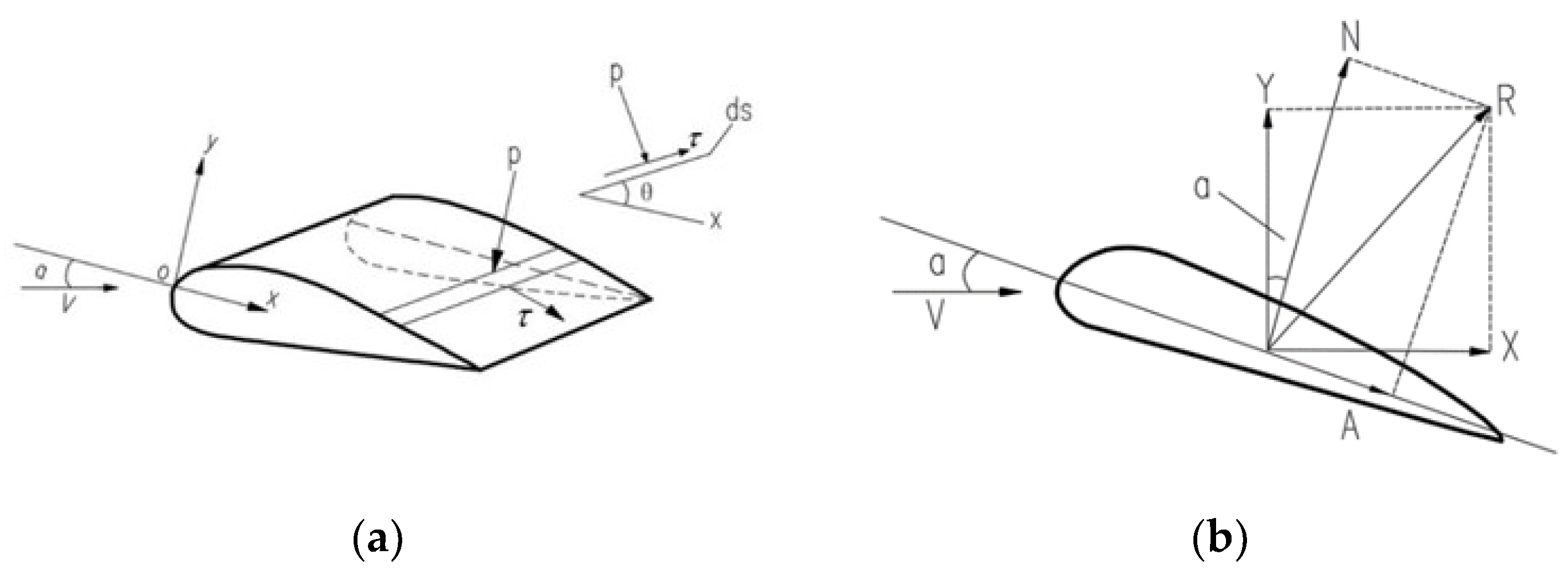
An airfoil generates varying pressures on its upper and lower surfaces under the action of an airflow. The force analysis diagram for an airfoil is shown in Figure 1. In the airfoil plane, the angle between the freestream velocity V and the airfoil chord line is defined as the geometric angle of attack α, and the pressure and frictional shear stresses on the airfoil surface generate a resultant force R, which can be resolved into a component N perpendicular to the chord line and a component A parallel to the chord line.

Figure 1.
Airfoil force analysis diagram: (a) airfoil surface pressure and friction shear stresses; (b) airfoil lift drag and synthesis.
The normal force N, axial force A, and resultant force R are defined in Equation (1).
where: P is the pressure perpendicular to the airfoil surface, τ is the frictional shear stress tangent to the airfoil surface
Lift Y and drag X are defined in Equation (2).
To study the two-dimensional aerodynamic properties, an airfoil is approximated as an infinitely long wing in the spanwise direction. In this approximation, the aerodynamic forces of an airfoil at any cross-section of the wing could be represented by two-dimensional data. However, in reality, both airplane wings and wind turbine blades have finite lengths, and the aerodynamic forces acting on any airfoil section are influenced by the air circulation at the spanwise cutoff, which exhibits distinct three-dimensional characteristics. By correcting the angle of attack using the wing trailing vortex system, localized two-dimensional aerodynamic data can be effectively combined with wind tunnel experimental data to calibrate and design wings or blades [31].
2.2. Blade Element Momentum Theory
Wind turbine blades are analyzed by considering blade elements (or foliations) of radius r and length dr. Bernoulli’s principle states that the pressure is lower in regions of higher flow velocity and higher in regions of lower flow velocity within the airflow field. Under relative motion between the element and the airflow, lift and drag forces are generated on the element, with drag aligned with the relative velocity direction and lift perpendicular to it. Furthermore, the resultant force R generates a moment about the airfoil’s aerodynamic center, known as the pitching moment. The angle between the relative airflow direction and the geometric chord of the blade airfoil was known as the angle of attack. Blade Element Momentum (BEM) theory [31] combines momentum conservation and blade element aerodynamics to analyze wind turbine performance. The key equations are derived as follows:
For a blade element at radial position r, the axial induction factor a and tangential induction factor a′ are defined by:
where
ø: Inflow angle between relative wind velocity Vrel and the rotor plane.
Σ: Solidity ratio, σ = Bc/2πr (B: number of blades; c: local chord length).
Cl, Cd: Lift and drag coefficients of the blade element.
The aerodynamic forces on a blade element are calculated using local flow conditions:
Relative wind velocity:
Lift force L and drag force D:
where is the air density and dr is the element width.
The torque dQ and power dP generated by a blade element are:
where Ω is the rotor angular velocity.
Ice accretion on wind turbine blades alters the blade geometry, affecting the flow characteristics over the surface and consequently influencing aerodynamic performance. Within the BEM framework, key factors must be considered: Firstly, the shape and distribution of the ice have a significant impact on the aerodynamic performance of the blade. Ice morphology varies (e.g., cylindrical, spherical horns) and is often inhomogeneous, concentrating in specific regions. These factors modify the blade surface geometry, altering the aerodynamic characteristics along the airfoil. Secondly, ice thickness significantly impacts blade aerodynamic performance. Increased ice thickness increases the blade surface area and alters airflow patterns, thereby affecting the lift and drag forces.
Accounting for these factors, BEM theory provides a framework for predicting the aerodynamic performance of ice-covered blades. It enables the construction of mathematical models and numerical simulations to calculate the aerodynamic parameters (e.g., lift, drag) for ice-covered blades. These parameters facilitate the assessment of icing-induced performance degradation and provide insights for optimizing blade design and operational strategies. However, actual icing conditions are highly complex, and BEM represents a simplified model of the phenomenon. Consequently, practical research requires combining experimental and numerical simulation methods to gain a comprehensive understanding of the blade icing impacts on wind turbine performance.
2.3. Similarity Theory
By Newton’s law of internal friction:
F: Viscous forces (in fluid mechanics);
μ: Dynamic viscosity of the fluid;
A: Area of internal friction action;
dy: Thickness of friction layer;
dv/dy: Velocity gradient.
Requiring that the viscous forces between the prototype and the model are satisfied to be similar, we have
v: Kinematic viscosity of the fluid.
Viscous force similarity requires that the prototype and model satisfy the following:
Vm: Kinematic viscosity of the model;
lm: Feature lengths of the model.
Then, it is required to satisfy Re equality between the prototype and the model, i.e., the viscous force similarity criterion, also known as the Reynolds criterion [32].
3. Numerical Simulation of Wind Turbine Blade Surface Ice Coverage
3.1. NACA0012 Airfoil Boundary Conditions and Meshing
The NACA0012 airfoil was utilized as the prototype for the experimental model, which has the following curve equations:
The upper surface of the airfoil is defined by the following equation [33]:
The lower surface of the airfoil is defined by the following equation:
To ensure accuracy in modeling ice accretion, three numerical simulation cases for the NACA0012 airfoil were designed, as detailed in Table 1. An airfoil chord length of 0.5334 m, consistent with the NASA test airfoil [26], was used. The ambient temperatures of −5.56 °C, −11.11 °C, and −26.11 °C were selected, and the ice types of glaze ice, rime ice, and mixed ice were fully considered. Model I features leading-edge glaze ice, Model II features leading-edge mixed ice, and Model III features leading-edge rime ice.

Table 1.
NACA0012 surface icing design conditions.
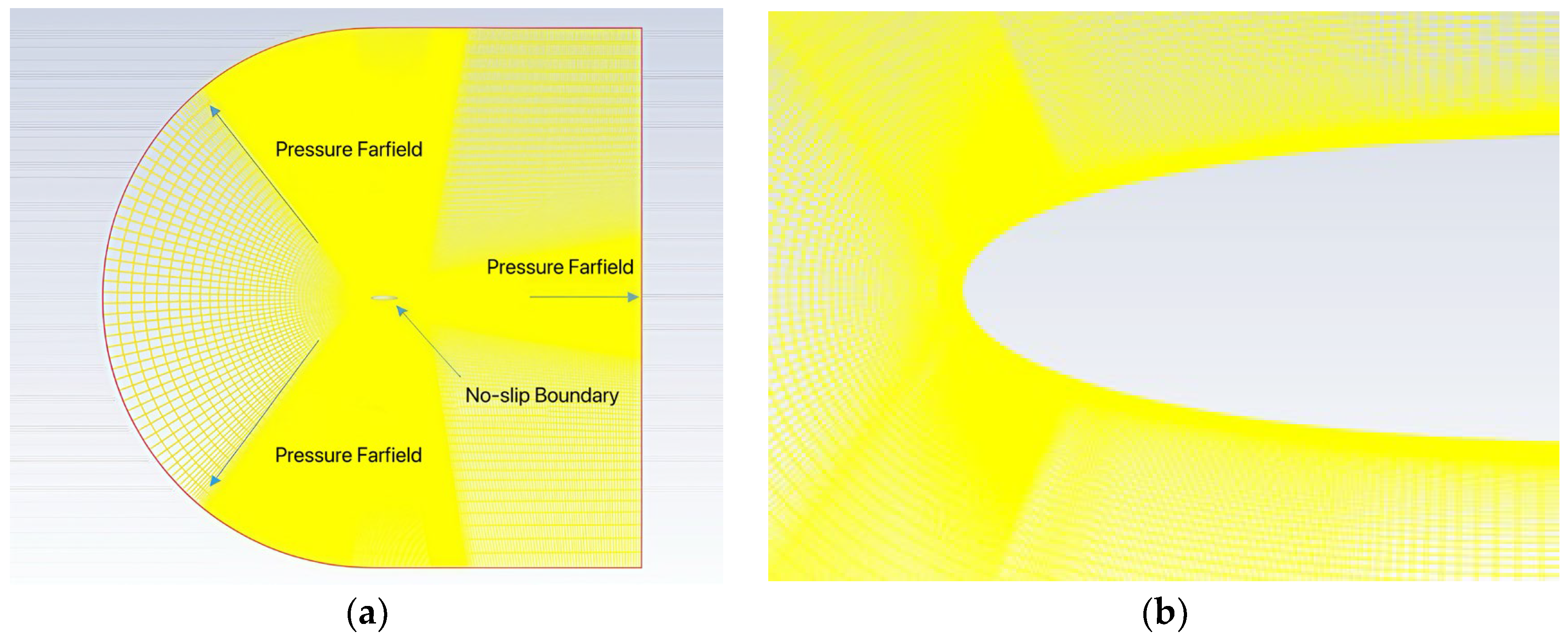
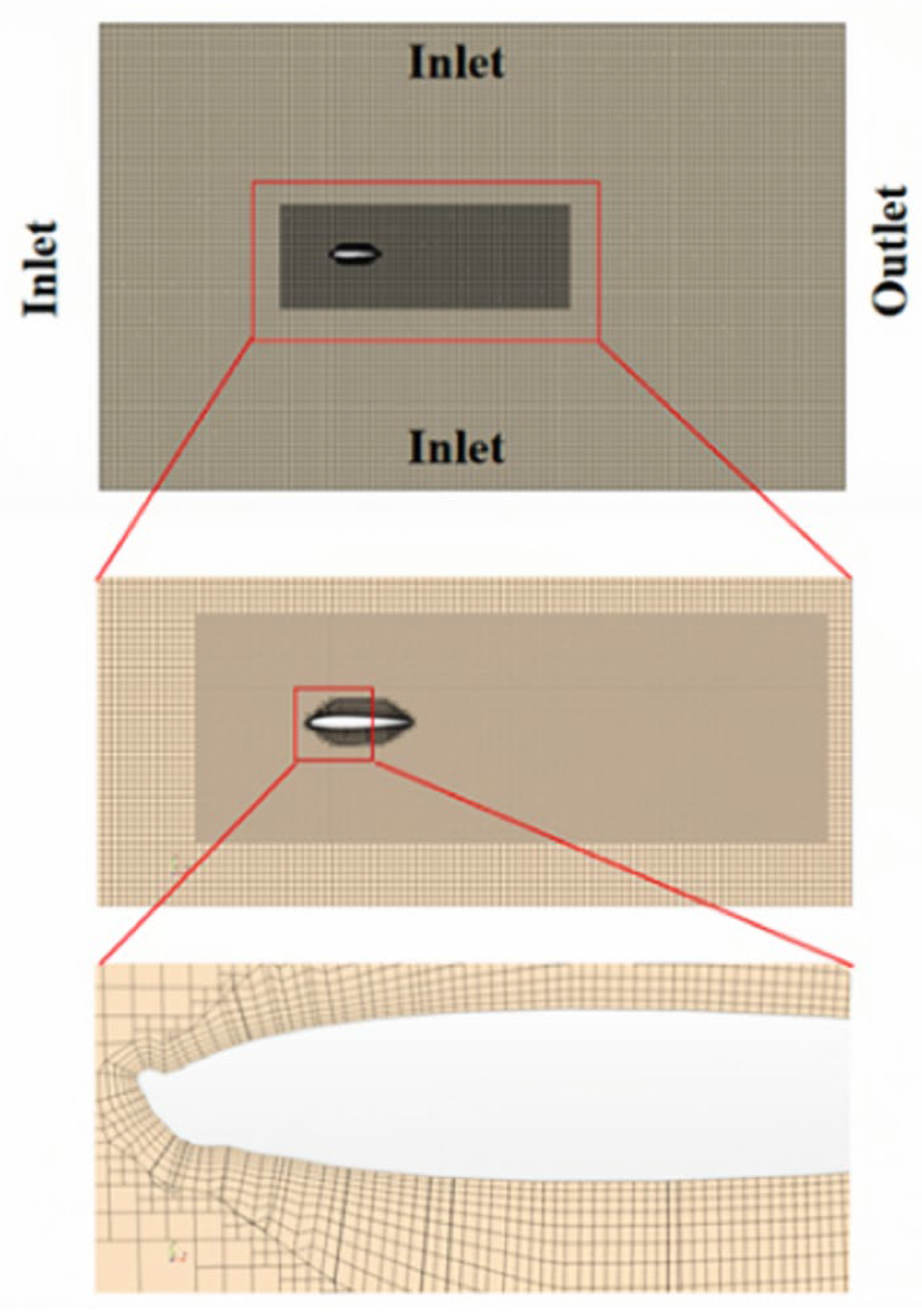
As shown in Figure 2a, the boundary conditions were set as follows: the curved left boundary, upper boundary, lower boundary, and right boundary were pressure farfields; boundaries perpendicular to the plane (front/rear) were symmetry planes; and the airfoil surface was a no-slip wall. To prevent backflow at the outlet, the outlet boundary was positioned more than 15 chord lengths downstream of the trailing edge. Due to the constant airfoil profile in the spanwise direction, only one cell layer (2 mm thick) was used in that direction. The height of the first cell layer adjacent to the airfoil wall was 0.001 mm, ensuring y+ < 1 for all conditions. The near-wall mesh is shown in Figure 2b.
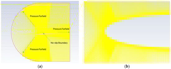
Figure 2.
Airfoil computational domain and meshing: (a) calculation domain and boundary conditions; (b) airfoil computational domain and meshing.
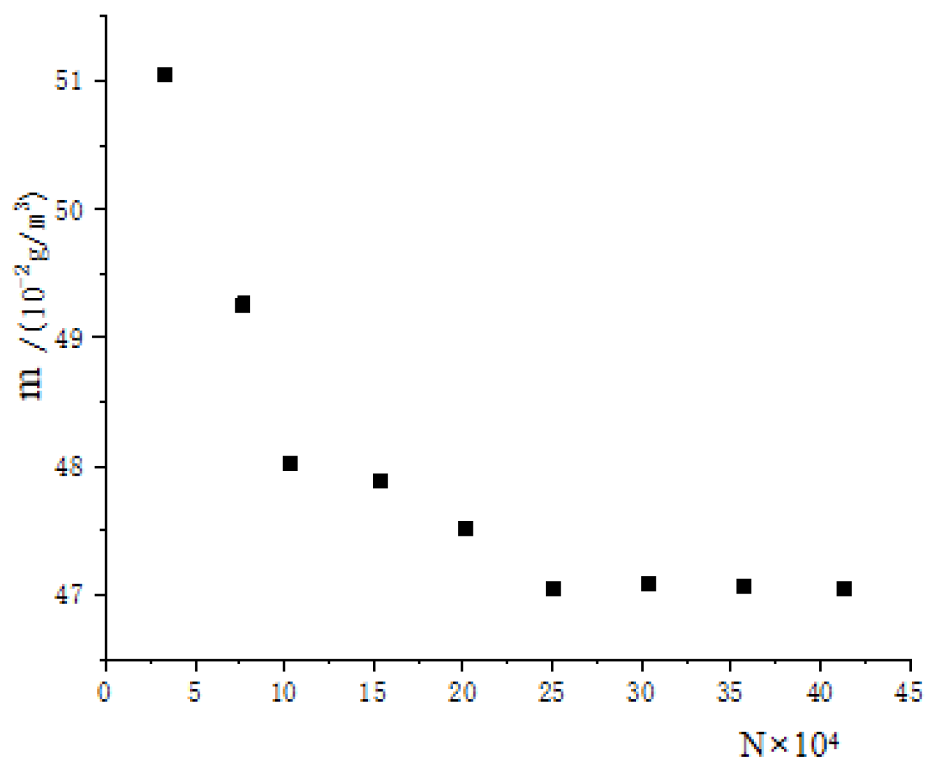
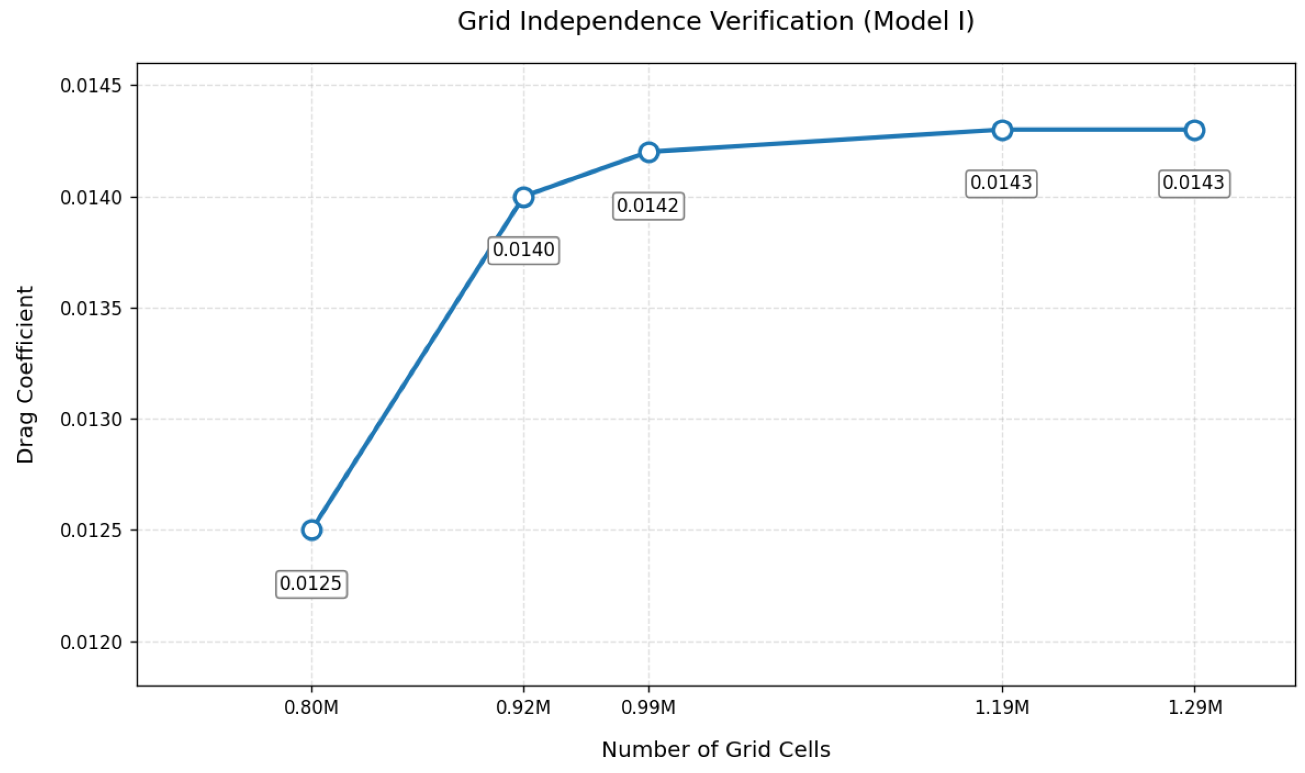
The mesh quality and density determine computational accuracy and efficiency. To ensure accuracy while minimizing computational cost, a grid independence study was conducted for Model I. The effect of cell count on predicted ice mass is shown in Figure 3. Ice mass stabilized for grids exceeding 250,000 cells.
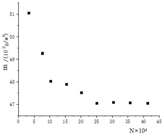
Figure 3.
Relationship between the number of grids and the mass of ice.
3.2. NACA0012 Wing Ice Cover Simulation Validation Study
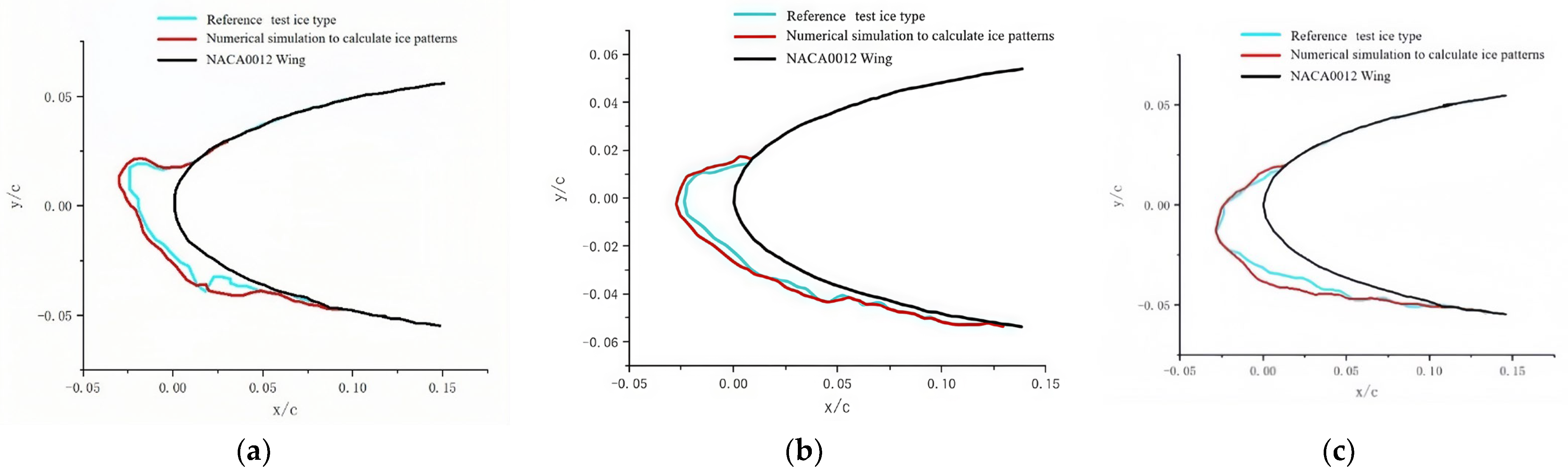
Ice accretion on the NACA0012 airfoil was simulated using ANSYS Fluent and FENSAP-ICE. The SST k-ω turbulence model was employed to resolve the flow field dynamics, while the shallow-water icing model was adopted to simulate ice accretion under varying thermodynamic conditions. Simulations clarified the accretion shapes for glaze, mixed, and rime ice types. The numerical results for the three models were compared with NASA icing test data [26], as shown in Figure 4 (c denotes chord length).
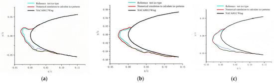
Figure 4.
Comparison of numerical simulation results with NASA test data: (a) Model I surface ice cover; (b) Model II surface ice cover; (c) Model III surface ice cover.
Figure 4 shows strong agreement between the simulated and experimental ice morphologies. The maximum ice thickness errors for the three models are summarized in Table 2. Notably, Model I exhibited a relatively higher maximum ice thickness error (7.98%). This discrepancy primarily stems from challenges in resolving droplet impingement dynamics—specifically, the interaction between supercooled droplets and the airfoil surface during accretion. The Navier–Stokes (N-S) equations, when coupled with icing thermodynamics, inherently involve simplifications in modeling droplet impingement efficiency and phase-change heat transfer, which can lead to localized inaccuracies in predicting ice growth near the leading edge. Despite this, the overall error remained acceptable, validating the numerical framework’s robustness for engineering applications.
Table 2.
Relative error of numerical simulation of maximum ice thickness.
4. Experimental Methodology for Aerodynamic Performance Assessment
4.1. Experimental Equipment
As shown in Figure 5, the DC wind tunnel system comprised four sections: the rectifier section, the experimental section, the transition section, and the fan section. The overall dimensions of the wind tunnel were 5.2 m (L) × 2.0 m (W) × 2.5 m (H), and the dimensions of the experimental section were 1500 mm (L) × 1000 mm (W) × 800 mm (H), with the effective size of the experimental section being 1200 mm (L) × 800 mm (W) × 600 mm (H). The range of experimental wind speed was from 0 m/s to 35 m/s, and the error of the anemometer was ±0.15 m/s or less. The uniformity of the flow field was ≤1.0%, the stability of the flow field was ≤0.5%, and the turbulence was ≤1.0%. Throughout the experiment, the air temperature was maintained at 16.4 °C, and the air density was 1.22 Kg/m3. Since the air inlet was composed of a honeycomb net and smooth walls, the airflow was treated as uniform along the height direction.
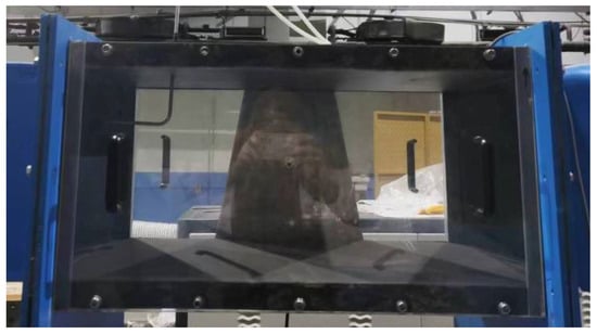
Figure 5.
Direct flow wind tunnel test equipment.
As shown in Figure 5, the DC wind tunnel system incorporated four integrated subsystems:
- 1.
- Test section (1500 × 1000 × 800 mm) with optically transparent walls for flow visualization (Evonik, Germany).
- 2.
- Force measurement: 6-axis transducer (ATI Gamma SI-130-10) with pitch control mechanism (±30°, 0.1° resolution).
- 3.
- PIV system: Dual-cavity Nd: YAG laser (532 nm) (ATI Gamma SI-130-10) and 4MP CCD camera (LaVision Imager Pro X) synchronized via programmable timing unit (LaVision GmbH, Göttingen, Germany).
- 4.
- Data acquisition: NI PXIe-1071 chassis (10 kHz sampling) (National Instruments (NI), Austin, TA, USA).
The experimental setup described qualifies as a wind tunnel due to its structural and functional alignment 4.1 with standardized aerodynamic testing principles. A wind tunnel is defined by its ability to generate controlled airflow for simulating real-world conditions, which this DC (direct-flow) system achieves through four key components: the rectifier section (equipped with a honeycomb mesh and smooth walls to eliminate turbulence and ensure uniform inflow), the experimental section (dimensions 700 mm × 400 mm × 300 mm, effective test area 600 mm × 320 mm × 240 mm), the transition section (minimizing flow disturbances between segments), and the fan section (providing adjustable velocities of 0–35 m/s). Flow quality is rigorously maintained, with uniformity ≤ 1.0%, stability ≤ 0.5%, and turbulence intensity ≤ 1.0%, ensuring precise aerodynamic measurements. Environmental control measures, including constant air temperature and density, isolate the icing effects from thermodynamic variability, while the anemometer accuracy enables detection of subtle aerodynamic changes.
4.2. Experimental Model
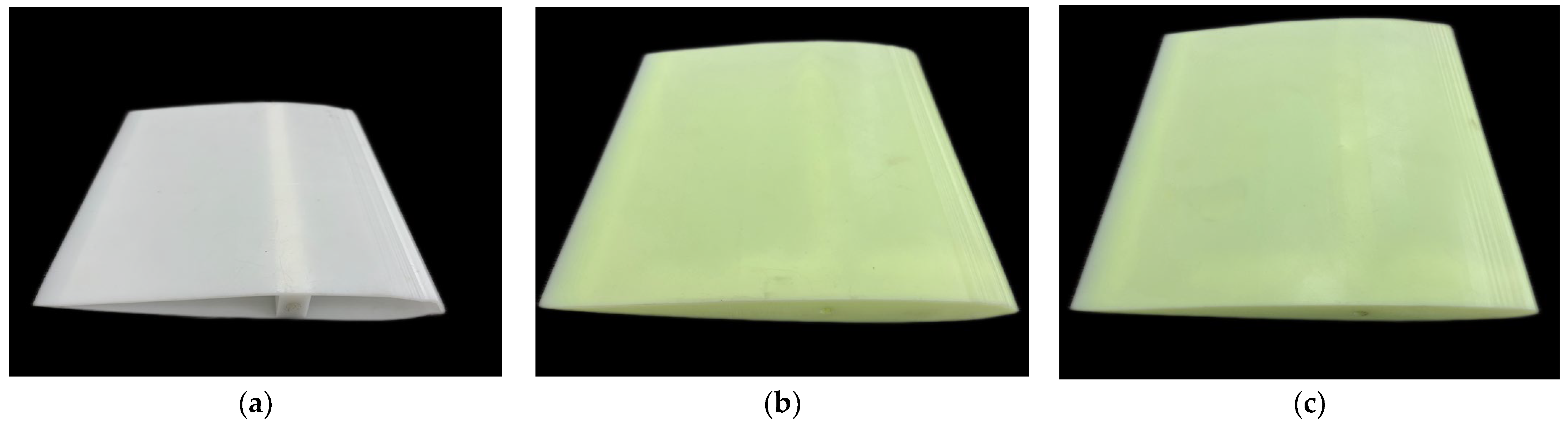
The experimental models were fabricated using 3D printing technology with a specialized resin material to replicate three distinct leading-edge ice accretion morphologies: glaze ice (smooth, transparent ice with sharp protrusions), mixed ice (a heterogeneous combination of glaze and rime ice forming irregular ridges), and rime ice (opaque, granular ice with a porous surface texture).
As shown in Figure 6, each model maintained a chord length of 0.2 m and a spanwise length of 0.2 m. Vertical holes (6 mm diameter) were drilled at the center of gravity of each model to secure them to force sensors via threaded rods. These sensors, connected to a data acquisition system, enabled real-time monitoring and recording of lift and drag forces during wind tunnel testing.

Figure 6.
Ice model experimental figure: (a) Model I experimental figure; (b) Model II experimental figure; (c) Model III experimental figure.
4.3. Design of Experimental Conditions
According to the Reynolds expression:
where
: Incoming flow velocity;
: Characteristic length;
: Kinematic viscosity.
Experimental measurements showed that the ambient laboratory temperature was maintained at 16.4 °C, with a corresponding air kinematic temperature of 16.4 °C. The target Reynolds number was calculated from the chord length to determine the wind speed required for dynamic similarity. Substituting these parameters into the equation yields the experimental wind speed. However, due to limitations in the wind tunnel’s operational range (maximum 35 m/s), this study adopted a scaled Reynolds similarity approach. As summarized in Table 3, adjusted wind speeds for each model (I–III) were derived by accounting for the temperature-dependent variations in air viscosity.
Table 3.
Simulated icing conditions and derived experimental parameters.
Based on the parameter settings in the table above, the appropriate experimental wind speed was determined. However, due to the limitation of the wind speed range of the DC wind tunnel equipment, which could provide a maximum wind speed of 35 m/s, this limitation was considered. This paper was based on the principle of similarity and with reference to the theory of the self-modeling zone.
When the Reynolds number of the fluid medium reached the order of 105, it was in the turbulent layer. Within this region, the kinematic properties of the fluid flow showed remarkable similarity. In the real situation against which the current experiments were benchmarked, the Reynolds number was on the order of 106, and the fluid exhibited both turbulent and laminar flow. However, the experimental conditions made it difficult to carry out physical property studies at this level. Therefore, the approach of simulating the turbulent layer properties was taken by limiting the Reynolds number of the air in the environment in which the model was located to the order of 105, in order to perform the simulation study.
Through detailed calculations, it was concluded that the Reynolds number limitations were satisfied when the wind speed exceeded 10 m/s, thus meeting the experimental requirements. All aerodynamic measurements account for potential blockage effects through established correction protocols. Considering the range of the small wind tunnel equipment, the range of experimental wind speed was finally determined to be between 10 m/s and 15 m/s. The experimental conditions are summarized in Table 4. This adjustment not only ensured the feasibility of the experiment but also maximized the reliability of the experimental results under the restricted conditions. This approach, based on the simulation of turbulent layer properties, provided a reasonable and practical solution for effectively conducting the experiment.
Table 4.
Summary of experimental conditions.
5. Aerodynamic Performance Analysis Based on Numerical Simulation
Numerical Methods
In this paper, the software Star-ccm+ (Version 17.06.012; Siemens Digital Industries Software) was applied to analyze the effect of different types of ice cover on the surface of a wind turbine blade on its aerodynamic performance. Appropriate computational meshes were generated based on the geometric parameters of the airfoil [22]. No-slip wall conditions were set as boundary conditions on the blade surface. The k-ε turbulence model was adopted, utilizing the robust performance of the SST k-ω model near walls to capture the viscous sublayer flow while applying the standard k-ε model in the core flow region to simulate the airflow field. The flow domain constructed for the airfoil was rectangular and based on existing studies in the literature [30]; the computational domain dimensions were set as follows: the inlet boundary was positioned 15 chord lengths (15c) upstream of the leading edge, the outlet boundary 20 chord lengths (20c) downstream of the trailing edge, and the top/bottom boundaries 10 chord lengths (10c) from the airfoil surface. The velocity inlet was located at 5 times the model chord length in front of the leading edge of the airfoil, and the pressure outlet was located at about 10 times the model chord length behind the trailing edge of the airfoil. The upper and lower surface distances from the model of the computed flow domains were both 5 times the model chord length to ensure that there was no backflow phenomenon in the flow field computation. The length of the flow field encrypted in the transverse direction was 6 times the chord length of the model. In order to accurately analyze the gas flow on the surface of the airfoil, a total of 10 prismatic layers were provided, and the expansion ratio of prismatic layers was 1.2. The surface of the airfoil was normal to the airfoil, and the minimum mesh spacing, Y+, was less than 1. Taking Model I as an example, the computational domain and mesh setup are shown in Figure 7.
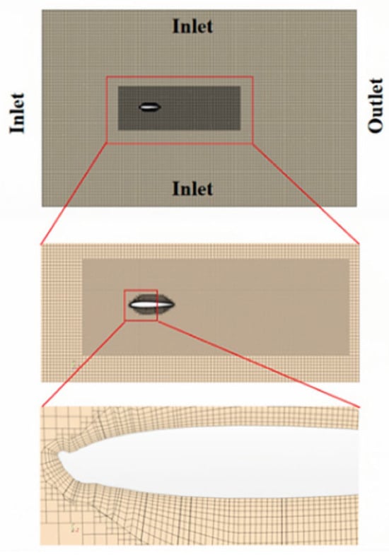
Figure 7.
Model I computational domain and mesh setting.
Considering that the three ice-covering models had only minor differences in the leading-edge part, and in the meshing stage, the number of meshes for the three models were 917,286, 916,828, and 916,643 with the basic size of 0.05 m, respectively; the differences were negligible. Therefore, in the mesh-independence verification stage, Model I was taken as an example for elaboration. Model I based on the resistance and the basic size of the mesh is shown in Figure 8.
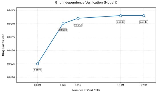
Figure 8.
Resistance-based grid independence verification.
According to Figure 8, the airfoil drag corresponding to different numbers of grids appeared to change, and the magnitude of the change in airfoil drag gradually decreased after the number of grids reached 917,286. In addition, the differences between the drag values corresponding to neighboring grid numbers were less than 5%. It meant that the accuracy of the numerical simulation was fully guaranteed within this range. Considering the guarantee of computational efficiency, a grid generation scheme with a basic size of 0.05 m was chosen for this simulation. This choice could guarantee the accuracy of the simulation results as well as the efficiency of the calculation.
6. Effect of Icing on Wind Turbine Output Power
6.1. Effect of Airfoil Ice Cover on Airfoil Surface Pressure Coefficients
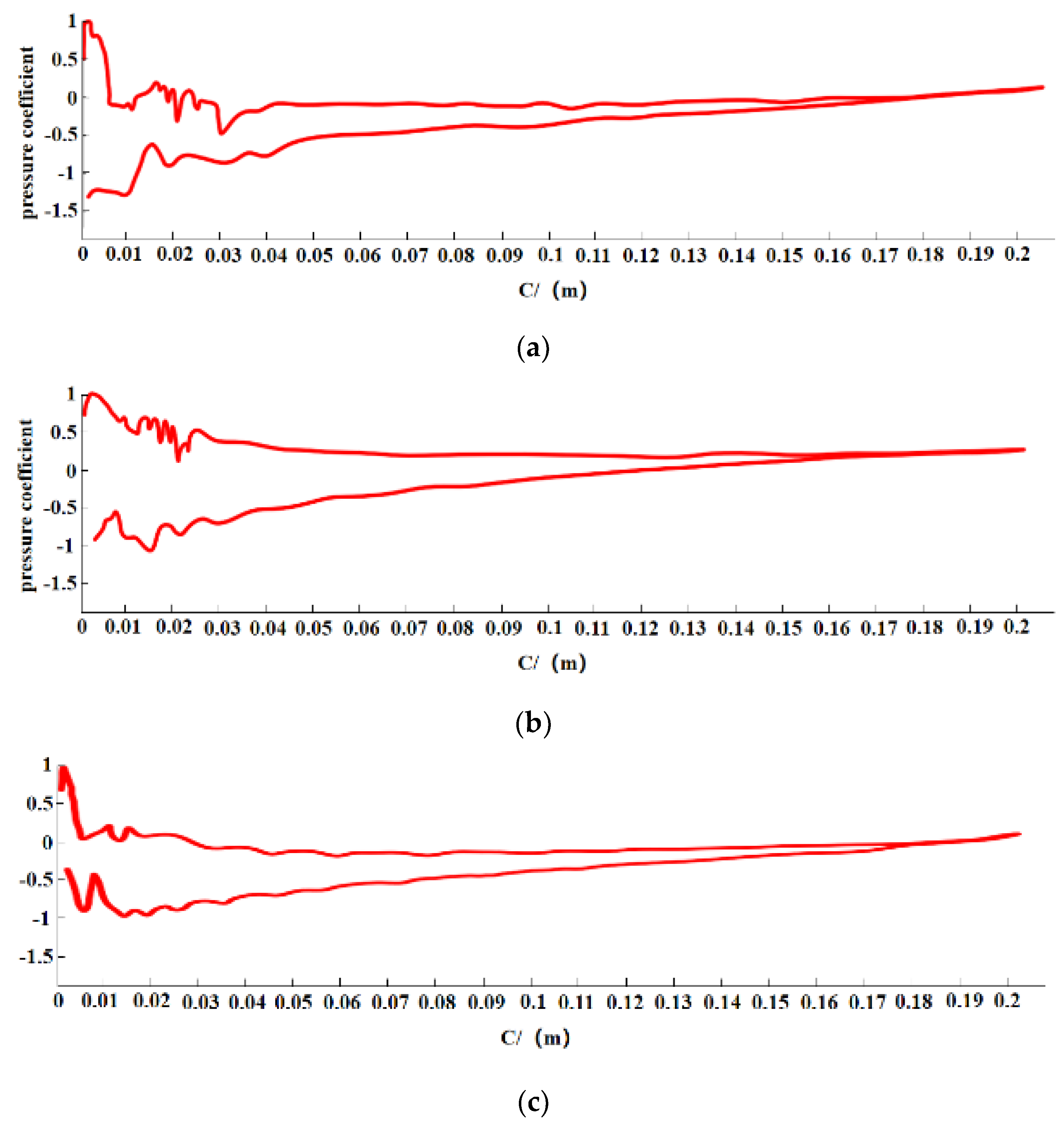
Icing on the leading edge of an airfoil significantly affected the airfoil surface pressure distribution and hence the aerodynamic performance of the airfoil. This effect was due to the presence of ice altering the airflow near the airfoil surface, which led to a change in the pressure coefficient distribution. The pressure coefficients at the leading edge of the airfoil appeared to oscillate after icing compared to the clean airfoil. As an example, the distribution of the pressure coefficients along the airfoil surface for Model I, Model II, and Model III at a base velocity of 10 m/s for the incoming flow velocity of 10 m/s is shown in Figure 9.
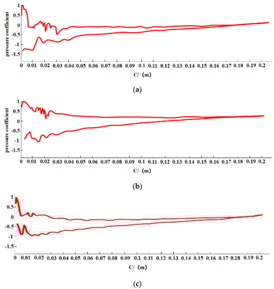
Figure 9.
The pressure coefficient is distributed along the surface of the airfoil: (a) Distribution of pressure coefficients along the airfoil surface for Model I; (b) distribution of pressure coefficients along the airfoil surface for Model II; (c) distribution of pressure coefficients along the airfoil surface for Model III.
The pressure coefficients at the leading edge of the airfoil all exhibited a significant irregular agitation phenomenon when glaze ice, mixed ice, and rime ice were attached to the leading edge of the airfoil. This phenomenon was mainly due to the fact that the ice overlay caused significant geometric irregularities at the leading edge of the airfoil, which increased the surface roughness and thus triggered the pressure coefficient agitation phenomenon. Among the three ice-covered cases, the effect of open ice on the leading edge of the airfoil was the most significant, leading to the most serious irregular oscillations in the pressure coefficient.
6.2. Effect of Airfoil Ice Cover on Airfoil Flow Field
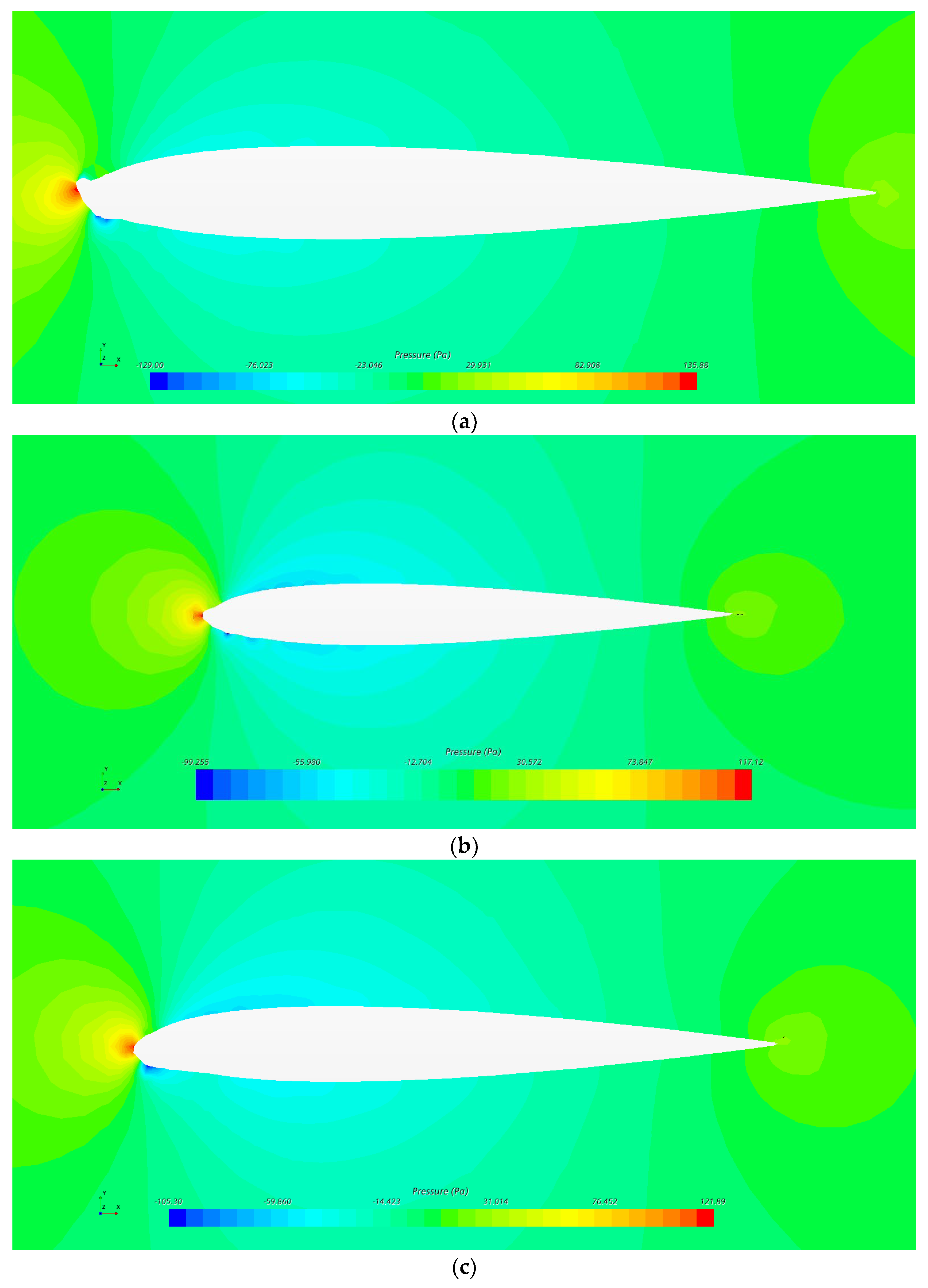
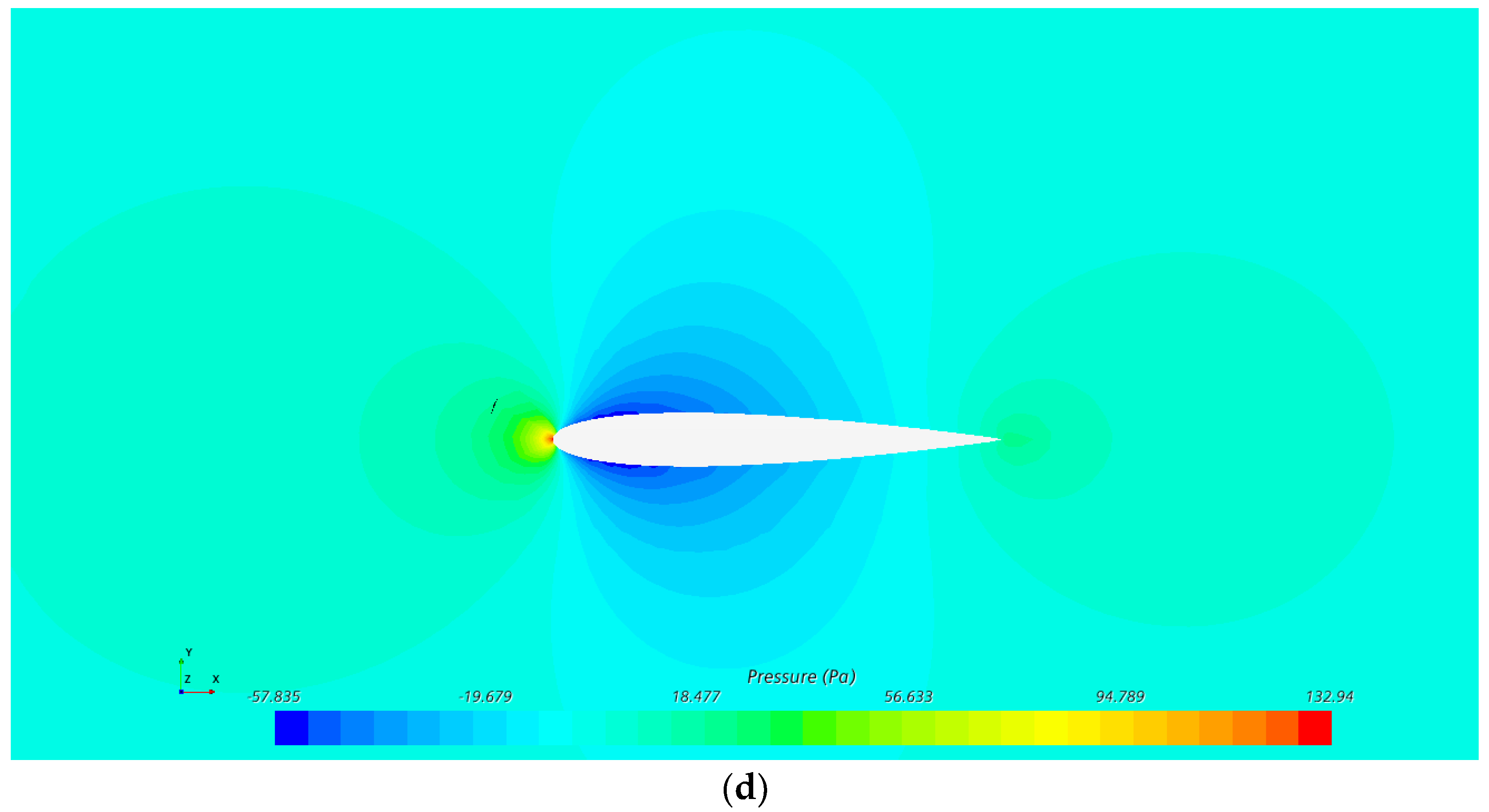
Icing on the leading edge of the airfoil caused the airflow to separate near the leading edge of the airfoil, and the location and nature of the separation point changed due to the presence of ice, which affected the flow pattern of the airflow on the surface of the airfoil. Pressure cloud plots of Model I, Model II, Model III, and the original model at 15 m/s are shown in Figure 10.

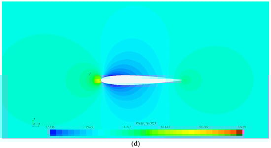
Figure 10.
Pressure image of ice-cover models and original model at incoming flow velocity of 15 m·s−1: (a) Model I pressure at an incoming flow rate of 15 m/s; (b) Model II pressure at an incoming flow rate of 15 m/s; (c) Model III Pressure at an incoming flow rate of 15 m/s; (d) pressure for the original model at an incoming velocity of 15 m/s.
Separation flow occurred when the airflow was stripped from the airfoil surface, and it was exacerbated by the increased surface roughness caused by the ice-covered airfoil, as well as by the resulting shape changes. The inability of the fluid to flow tightly over the airfoil surface created a large separation region and increased the resistance of the airfoil. Separation flow produced unsteady turbulent flow on the surface of the airfoil, exacerbating the generation of aerodynamic noise. As analyzed in Figure 10, the velocity distribution on the upper and lower surfaces of the un-iced airfoil was more uniform, and the aerodynamic characteristics of the airfoil were more stable. The maximum velocity of the iced airfoil appeared at the leading edge of the airfoil, which generated uneven air flow on the upper and lower surfaces of the airfoil, resulting in an increase in drag and a decrease in lift of the airfoil. At the same time, the ice-covered airfoil had a separation vortex at the tail. Both the separation of flow and the generation of vortex weakened the lift generation.
6.3. Effect of Wing Ice Cover on Wing Lift Coefficient of Resistance
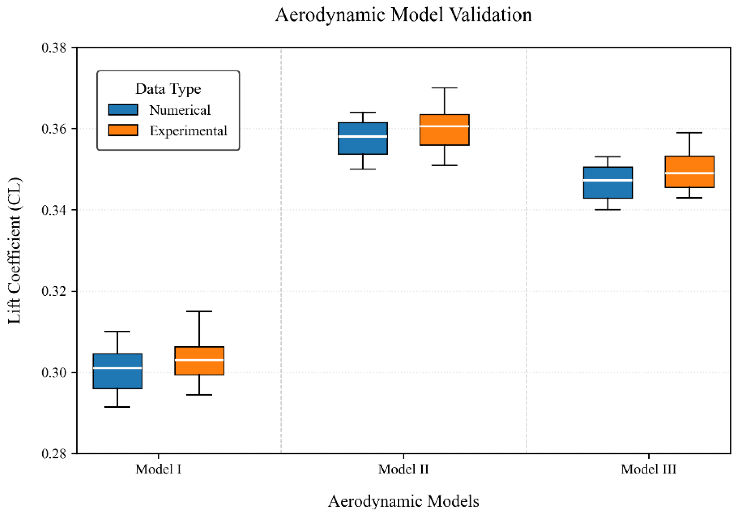
The lift coefficients for the three ice-covered models and clean airfoils at different incoming velocities are shown in Figure 11, and the drag coefficients are shown in Figure 12.
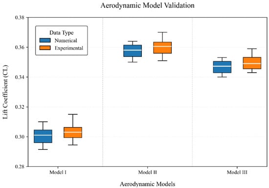
Figure 11.
Lift coefficient of ice-covered models at different incoming flow speeds.
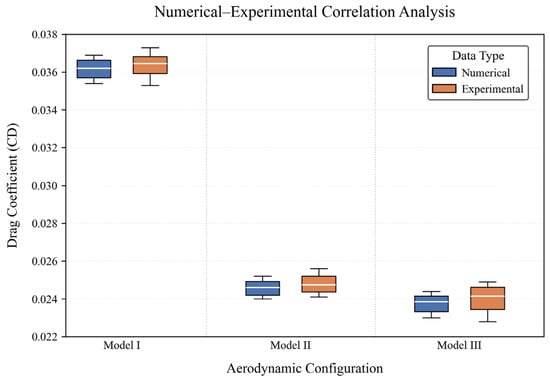
Figure 12.
Drag coefficient of ice-covered models at different incoming flow speeds.
Most experimental results showed higher values than numerical simulation results, yet the trends of the two were roughly consistent, indicating a certain degree of agreement between numerical simulations and experiments. Numerical simulations typically rely on a series of physical models and simplifying assumptions, whereas experiments are affected by factors such as wind tunnel equipment limitations and model imperfections. Experimental data incorporate adjustments for wind tunnel blockage effects to ensure validity.
Analysis suggests that this outcome may be attributed to the lateral stability of the model being compromised by incoming flow velocity fluctuations during experimentation. Uncontrolled deflections of the model, induced by variations in flow velocity, interfered with the precise measurement of the lift–drag coefficients. Notably, while the experimental results exceeded numerical simulation predictions, the congruence in trends validates the consistency between model experiments and computational modeling while underscoring the critical importance of flow velocity stability in wind tunnel testing.
Airfoil icing alters the leading-edge airflow separation point by modifying the surface geometry. Ice accretion on the airfoil leading edge introduces localized topological changes, promoting premature airflow separation at the surface and expanding the boundary layer separation zone. This phenomenon results in lift degradation and drag augmentation, as the enlarged separation area disrupts coherent flow attachment.
Concurrently, the high-velocity region on the airfoil surface shifts forward, with the velocity maximum occurring at the ice-covered leading edge—particularly at angular protrusions formed by ice overlay. In the wake region, separation vortices develop, further attenuating lift generation. Both flow separation and vortex shedding disrupt the aerodynamic loading consistency, leading to reduced energy capture efficiency.
As shown in Figure 11 and Figure 12, the attachment of glaze ice to the airfoil leading edge results in the most irregular ice pattern, which has the greatest impact on the airfoil’s aerodynamic performance: at an incoming velocity of 10 m/s, the lift coefficient decreases by 34.9% and the drag coefficient increases by 97.2% under glaze ice conditions, while mixed ice causes a 33.6% lift reduction and a 22.7% drag increase, and rime ice leads to a 24.1% lift decrease and a 27.2% drag augmentation.
6.4. Effect of Wing Ice Cover on Wind Energy Utilization Factor of Wind Turbines
Ice cover on the surface of wind turbine blades led to a reduction in the power output of the wind turbine due to a decrease in lift and an increase in drag. Ice cover on the blades led to a change in the optimum tip speed ratio of the wind turbine, which prevented the wind turbine from operating at its optimum operating point. The effect of ice cover on the output power of the wind turbine could be described by the following mathematical model.
Pice: Wind turbine output after ice cover;
Cpice: Wind energy utilization factor for wind turbines after ice cover;
ρ: Air density in Kg/m3;
A: Area swept by the blade in m2;
v: Incoming velocity in m/s.
Wind Turbine Wind Energy Utilization Coefficient is a dimensionless parameter that describes the efficiency of a wind turbine in capturing energy from the wind, and is an important indicator of the performance of a wind turbine. The wind energy utilization factor is expressed through the lift coefficient Cl and the drag coefficient Cd when considering the airfoil characteristics.
λ is the wing tip speed ratio; according to relevant information, the tip speed ratio of large horizontal axis wind turbines is usually designed around 8.
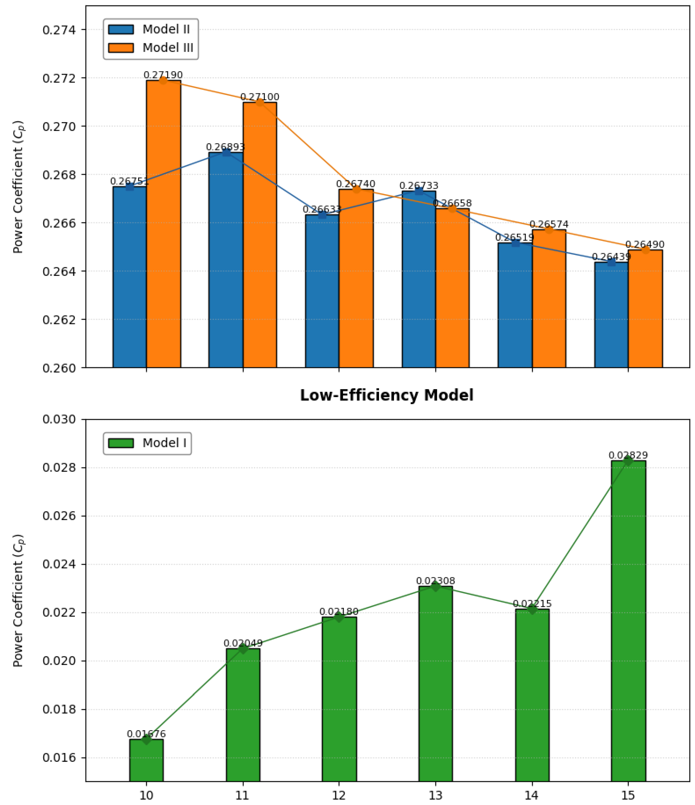
In this study, the wind energy utilization factors of three ice-cover models were compared under wind speeds ranging from 10 m/s to 15 m/s. In Figure 13, the results showed that Model I had the worst performance of wind energy utilization coefficients at all ambient wind speeds. Comparatively, the wind energy utilization coefficients of Model II and Model III were more consistent with each other, and both were stable in the range of 0.26 to 0.28. Specifically, the average increase in the wind energy utilization coefficient Cp for Model II compared to Model I was 91.71%, while the average increase in the wind energy utilization coefficient Cp for Model III compared to Model I was 91.74%. These data indicated that Model II and Model III had significant advantages in wind energy utilization efficiency under ice-covered conditions.
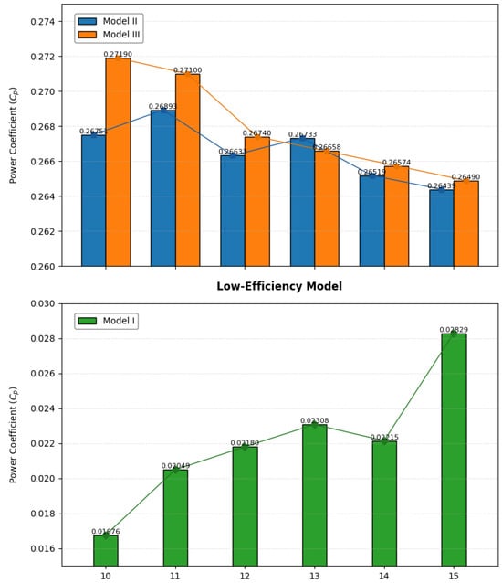
Figure 13.
Wind energy utilization factor for three ice-cover models.
By statistically analyzing the wind energy utilization coefficients of the three models, it was found that the wind energy utilization coefficients of Model I were lower and that their degree of dispersion was relatively high, with the ratio of the standard deviation to the mean being 17.0%, indicating that their data fluctuated a lot. The wind energy utilization coefficients of Model II and Model III were higher, and their degree of dispersion was lower, with the ratio of the standard deviation to the mean being 0.62% and 1.07%, respectively, indicating that the wind energy utilization coefficients of Model II and Model III were more stable under different wind speeds.
The above results showed that the wind energy utilization efficiency of Model I was significantly lower than that of Model II and Model III in ice-covered environments with wind speeds ranging from 10 m/s to 15 m/s. This indicated the poor energy conversion efficiency in the wind power generation process under ice-covered conditions for Model I. In contrast, Model II and Model III showed an average increase of 91.71% and 91.74%, respectively, indicating that these two ice-covered models had better wind energy capture capability under the same environmental conditions.
7. Conclusions
This study comprehensively analyzes the aerodynamic performance of airfoils with leading-edge glaze, mixed, and rime ice accretion through integrated DC wind tunnel experiments and STAR-CCM+ simulations. Key findings from lift-drag coefficients, surface pressure distributions, flow field structures, and power coefficients (Cp) are summarized as follows:
- (1)
- Different types of ice cover have varying effects on airfoil aerodynamic performance, with the most significant impact occurring when ice is attached to the airfoil’s leading edge: at an incoming flow velocity of 10 m/s, glaze ice causes a 34.9% reduction in the airfoil’s lift coefficient and a 97.2% increase in the drag coefficient, accompanied by the most obvious and severe irregular fluctuations in the pressure coefficient at the leading edge due to its angular structure; mixed ice leads to a 33.6% lift coefficient decrease and a 22.7% drag coefficient increase, with moderate pressure coefficient agitation; rime ice results in a 24.1% lift coefficient reduction and a 27.2% drag coefficient increase, with relatively mild pressure coefficient fluctuations. The degree of pressure coefficient irregularity at the leading edge directly correlates with the geometric irregularity of the ice, highlighting that glaze ice with sharp protrusions has the most detrimental effect on aerodynamic performance.
- (2)
- Icing on the airfoil leading edge alters the airflow separation point by modifying the surface geometry, making it easier for airflow to separate from the airfoil surface. This shift in the separation point induces irregular pressure distributions across the airfoil, disrupting its aerodynamic characteristics. The velocity maximum occurs at the ice-covered leading edge—particularly at angular protrusions formed by ice—while separation vortices develop at the trailing edge. Both flow separation and vortex generation diminish lift production by disrupting coherent flow attachment and the pressure differential across the airfoil.
- (3)
- Through an analysis of the wind energy utilization coefficient (Cp) values of three ice-covered airfoils, it was found that under identical environmental conditions, the Cp values were significantly lower for airfoils with glaze ice attached to the leading edge compared to those with rime ice or mixed ice. Specifically, in the wind speed range of 10–15 m/s, the Cp values for airfoils with rime ice and mixed ice on the leading edge were more consistent, stabilizing between 0.26 and 0.28. Notably, the average Cp of airfoils with mixed ice on the leading edge increased by 91.71% compared to those with glaze ice, while the average Cp of airfoils with rime ice increased by 91.74% compared to those with glaze ice. These results highlight the critical impact of ice morphology on the wind energy capture efficiency, with rime and mixed ice demonstrating superior aerodynamic performance over glaze ice in cold-flow environments.
This paper investigates blade icing impacts through model testing and numerical simulations. However, actual wind turbine operations involve complex multi-parameter interactions among external factors including the wind speed, humidity, and temperature that collectively influence icing formation and aerodynamic performance. Due to this inherent environmental complexity, the deterministic prediction of icing effects on power generation efficiency remains challenging through isolated modeling approaches. Consequently, our findings require field validation to ensure reliability, particularly given the methodological constraints involving Reynolds number scaling differences, static ice profile assumptions, and the exclusion of natural environmental cycling. Future research should incorporate operational turbine data capturing transient ice morphology with synchronous meteorological parameters to correlate with experimental and simulation results. Such validation will strengthen the credibility of icing impact mechanisms while enabling comprehensive power efficiency assessment.
Author Contributions
Methodology, C.L.; Software, H.W.; Writing—original draft, Y.J. and J.W.; Writing—review & editing, Y.L. and D.Z. All authors have read and agreed to the published version of the manuscript.
Funding
This work was supported by the National Key Research and Development Program of China (2024YFC2816304) and the High-tech marine scientific research projects (CBG2N21-2-2).
Data Availability Statement
The original contributions presented in this study are included in the article. Further inquiries can be directed to the corresponding author.
Conflicts of Interest
The authors declare no conflict of interest.
References
- Kim, C.; Dinh, M.-C.; Sung, H.-J.; Kim, K.-H.; Choi, J.-H.; Graber, L.; Yu, I.-K.; Park, M. Design, Implementation, and Evaluation of an Output Prediction Model of the 10 MW Floating Offshore Wind Turbine for a Digital Twin. Energies 2022, 15, 6329. [Google Scholar] [CrossRef]
- Clarke, L.; Wei, Y.-M.; De La Vega Navarro, A.; Garg, A.; Hahmann, A.N.; Khennas, S.; Azevedo, I.M.L.; Löschel, A.; Singh, A.K.; Steg, L.; et al. Chapter 6: Energy systems. In Climate Change 2022: Mitigation of Climate Change. Contribution of Working Group III to the Sixth Assessment Report of the Intergovernmental Panel on Climate Change; IPCC, Ed.; Cambridge University Press: Cambridge, UK, 2022; pp. 613–746. [Google Scholar]
- Gao, L.Y.; Hu, H. Wind turbine icing characteristics and icing-induced power losses to utility-scale wind turbines. Proc. Natl. Acad. Sci. USA 2021, 118, e2111461118. [Google Scholar] [CrossRef] [PubMed]
- Wallenius, T.; Lehtomäki, V. Overview of cold climate wind energy: Challenges, solutions, and future needs. Wiley Interdiscip. Rev. Energy Environ. 2015, 5, 128–135. [Google Scholar] [CrossRef]
- Villalpando, F.; Reggio, M.; Ilinca, A. Prediction of ice accretion and anti-icing heating power on wind turbine blades using standard commercial software. Energy 2016, 114, 1041–1052. [Google Scholar] [CrossRef]
- Manatbayev, R.; Baizhuma, Z.; Bolegenova, S.; Georgiev, A. Numerical simulations on static Vertical Axis Wind Turbine blade icing. Renewable Energy 2021, 170, 997–1007. [Google Scholar] [CrossRef]
- Son, C.; Kim, T. Development of an icing simulation code for rotating wind turbines. J. Wind. Eng. Ind. Aerodyn. 2020, 203, 104239. [Google Scholar] [CrossRef]
- Cao, H.; Bai, X.; Ma, X.; Yin, Q.; Yang, X.-Y. Numerical simulation of icing on NREL 5-MW reference offshore wind turbine blades under different icing conditions. China Ocean. Eng. 2022, 36, 767–780. [Google Scholar] [CrossRef]
- Kreutz, M.; Ait Alla, A.; Lütjen, M.; Ohlendorf, J.-H.; Freitag, M.; Thoben, K.-D.; Zimnol, F.; Greulich, A. Ice prediction for wind turbine rotor blades with time series data and a deep learning approach. Cold Reg. Sci. Technol. 2023, 206, 103741. [Google Scholar] [CrossRef]
- Ye, F.; Ezzat, A.A. Icing detection and prediction for wind turbines using multivariate sensor data and machine learning. Renew. Energy 2024, 231, 120879. [Google Scholar] [CrossRef]
- Cheng, T.; Tao, T.; Bai, X.; Liu, Y. A CNN-Attention-GRU-based model for ice accretion prediction on wind turbine blades. J. Renew. Sustain. Energy 2023, 15, 033301. [Google Scholar]
- Zhang, T.; Lian, Y.; Xu, Z.; Li, Y. Effects of Wind Speed and Heat Flux on De-icing Characteristics of Wind Turbine Blade Airfoil Surface. Coatings 2024, 14, 852. [Google Scholar] [CrossRef]
- Fahed, M.; Martini, F.; Ibrahim, H.; Rizk, P.; Ilinca, A. Quasi-3D modeling for ice accretion prediction on wind turbine blades. Wind. Energy Sci. 2022, 8, 123–134. [Google Scholar]
- Bazilevs, Y.; Hsu, M.-C.; Akkerman, I.; Wright, S.; Takizawa, K.; Henicke, B.; Spielman, T.; Tezduyar, T.E. 3D simulation of wind turbine rotors at full scale. Part I: Geometry modeling and aerodynamics. Int. J. Numer. Methods Fluids 2010, 65, 207–235. [Google Scholar] [CrossRef]
- Srinath, D.N.; Mittal, S. Optimal aerodynamic design of airfoils in unsteady viscous flows. Comput. Methods Appl. Mech. Eng. 2010, 199, 1976–1991. [Google Scholar] [CrossRef]
- Lagdani, O.; Tarfaoui, M.; Nachtane, M.; Trihi, M.; Laaouidi, H. A numerical investigation of the effects of ice accretion on the aerodynamic and structural behavior of offshore wind turbine blade. Wind. Eng. 2020, 45, 1433–1446. [Google Scholar] [CrossRef]
- Askan, A.; Tangöz, S.; Konar, M. An investigation of aerodynamic behaviours and aerodynamic performance of a model wing formed from different profiles. Aeronaut. J. 2023, 127, 676–697. [Google Scholar] [CrossRef]
- Chen, P.W.; Bai, C.J.; Wang, W.C. Experimental and numerical studies of low aspect ratio wing at critical Reynolds number. Eur. J. Mech. B-Fluids 2016, 59, 161–168. [Google Scholar] [CrossRef]
- Bragg, M.B.; Broeren, A.P.; Blumenthal, L.A. Iced-airfoil aerodynamics. Prog. Aerosp. Sci. 2005, 41, 323–362. [Google Scholar] [CrossRef]
- Blasco, P.; Palacios, J.; Schmitz, S. Effect of icing roughness on wind turbine power production. Wind Energy 2017, 20, 601–617. [Google Scholar] [CrossRef]
- Davis, N.N.; Pinson, P.; Hahmann, A.N.; Clausen, N.; Žagar, M. Identifying and characterizing the impact of turbine icing on wind farm power generation. Wind Energy 2016, 19, 1503–1518. [Google Scholar] [CrossRef]
- Zhang, Y.J.; Kehtarnavaz, N.; Rotea, M.; Dasari, T. Prediction of Icing on Wind Turbines Based on SCADA Data via Temporal Convolutional Network. Energies 2024, 17, 2175. [Google Scholar] [CrossRef]
- Scher, S.; Molinder, J. Machine learning-based prediction of icing-related wind power production loss. IEEE Access 2019, 7, 129421–129429. [Google Scholar] [CrossRef]
- Kreutz, M.; Ait-Alla, A.; Varasteh, K.; Oelker, S.; Greulich, A.; Freitag, M.; Thoben, K.-D. Machine learning-based icing prediction on wind turbines. Procedia CIRP 2019, 81, 423–428. [Google Scholar] [CrossRef]
- Chuang, Z.; Yi, H.; Chang, X.; Liu, H.; Zhang, H.; Xia, L. Comprehensive Analysis of the Impact of the Icing of Wind Turbine Blades on Power Loss in Cold Regions. J. Mar. Sci. Eng. 2023, 11, 1125. [Google Scholar] [CrossRef]
- Abbasi, S.; Mahmoodi, A.; Joodaki, A. A Numerical Study on Effects of Ice Formation on Vertical-axis Wind Turbine Performance and Flow Field at Optimal Tip Speed Ratio. J. Appl. Fluid Mech. 2024, 17, 1896–1911. [Google Scholar]
- Kollar, L.E.; Mishra, R. Inverse design of wind turbine blade sections for operation under icing conditions. Energy Convers. Manag. 2019, 180, 844–858. [Google Scholar] [CrossRef]
- ISO 12494; Atmospheric Icing of Structures. International Organization for Standardization: Geneva, Switzerland, 2001.
- IEC 61400-12-1; Wind Turbines—Part 12-1: Power Performance Measurements of Electricity Producing Wind Turbines. International Electrotechnical Commission: Geneva, Switzerland, 2005.
- Woebbeking, M.; Argyriadis, K. New guidelines for the certification of offshore wind turbines. In Proceedings of the International Ocean and Polar Engineering Conference, Anchorage, AK, USA, 30 June–5 July 2013. [Google Scholar]
- Cai, X.; Wang, H.; Wang, Y.; Xu, B.; Zheng, Y.; Zhang, L. (Eds.) Wind Power Generation Engineering Technology Series: Wind Turbine Blades, 2nd ed.; China Water & Power Press: Beijing, China, 2022. [Google Scholar]
- White, F.M. Fluid Mechanics, 8th ed.; McGraw-Hill: New York, NY, USA, 2016. [Google Scholar]
- Jacobs, E.N.; Ward, K.E.; Pinkerton, R.M. NACA Report No. 460: Characteristics of 78 Related Airfoil Sections; NACA: Washington, DC, USA, 1933. [Google Scholar]


Disclaimer/Publisher’s Note: The statements, opinions and data contained in all publications are solely those of the individual author(s) and contributor(s) and not of MDPI and/or the editor(s). MDPI and/or the editor(s) disclaim responsibility for any injury to people or property resulting from any ideas, methods, instructions or products referred to in the content. |
© 2025 by the authors. Licensee MDPI, Basel, Switzerland. This article is an open access article distributed under the terms and conditions of the Creative Commons Attribution (CC BY) license (https://creativecommons.org/licenses/by/4.0/).