Numerical Simulation of Treatment Capacity and Operating Limits of Alkali/Surfactant/Polymer (ASP) Flooding Produced Water Treatment Process in Oilfields

Abstract

As an enhanced oil recovery (EOR) technique, alkali/surfactant/polymer (ASP) flooding effectively mitigates production decline in mature oilfields through chemical flooding mechanisms. The breakthrough of ASP chemical agents poses challenges to the green and efficient separation of oilfield produced water. In this paper, sedimentation separation of produced water was simulated using the Eulerian method and the RNG k–ε model. In addition, the filtration process was simulated using a discrete phase model (DPM) and a porous media model. The distribution characteristics of oil/suspended solids obtained through simulation, along with the water quality parameters at each treatment node, were systematically extracted, and the influence of operating conditions on treatment capacity was analyzed. Simulations reveal that elevated treatment loads and produced water polymer concentrations synergistically impair ASP flooding produced water treatment efficiency. Fluctuations of operating conditions generate oil/suspended solids content in output water ranges spanning 13–78 mg/L and 19–92 mg/L, respectively. The interpolation method is adopted to determine the critical water quality parameters of each treatment node, ensuring that the treated produced water meets the treatment standards. The operating limits of the ASP flooding produced water treatment process are established.

1. Introduction

The mature oilfields exhibit the characteristics of formation energy attenuation and recovery rate decline [1,2]. Water flooding is the basic method to enhance oil recovery [3]. Based on water flooding, EOR has become the main method to tap the potential of remaining oil in mature oilfields [4,5]. For mature oilfields, chemical flooding technology represented by ASP flooding has been widely used [6,7,8]. This technology improves oil displacement efficiency by reducing oil–water interfacial tension, improving mobility ratio, and changing rock wettability through the synergistic action of alkali, surfactant, and polymer [8,9,10,11]. However, the breakthrough of ASP chemical agents complicates the produced water quality characteristics, leading to higher polymer concentrations, increased viscosity, and smaller oil droplet sizes [9,12,13,14]. Produced water contains crude oil, suspended solids, and various contaminants. Unrestricted discharge can lead to environmental pollution, while direct reinjection may result in formation plugging and affect oilfield development. Injecting treated produced water back into the formation is also a critical component of ASP flooding [15,16].

The produced water from ASP flooding is typically treated through a combined sedimentation and filtration process to ensure effective treatment and reinjection [17,18]. During sedimentation, oil, water, and suspended solids undergo preliminary separation based on their density differences. The efficiency of this separation depends on both water quality and treatment amount [19,20]. As the last step for produced water treatment, filtration critically determines reinjection water quality. During filtration, the filter material captures and adsorbs suspended particles, achieving further separation. The effect of filtration treatment is affected by the water quality characteristics, filtration rates, and filter material [17,20]. With the continuous innovation and application of oil recovery technology, oilfields adopt diversified treatment processes to deal with increasingly complex water quality. The air flotation method is adopted by some oilfields to treat produced water with strong oil–water stability and substantial emulsified oil content. By injecting dissolved gas into the produced water, dispersed bubbles drive the oil droplets to the surface for separation [21,22]. Utilizing the selective permeability of membranes, the membrane separation method effectively removes salts, organic compounds, and microorganisms in produced water [23,24]. The chemical separation method is to add flocculant, coagulant, and other chemical agents in the produced water, causing suspended solids in the water to gather to form a large flocculation for sedimentation [25,26].

As the main method for studying sedimentation and filtration processes, Computational Fluid Dynamics (CFD) can study the flow process of fluid in sedimentation and filtration tanks, and has become an important method for the design and optimization of wastewater treatment processes. Liu et al. studied the liquid–solid two-phase turbulent flow in a sedimentation tank using the CFD method, and obtained the influence of liquid flow state on the sedimentation process [27]. Tarpugkou et al. adopted a Lagrangian approach to simulate two-way liquid–solid coupling with momentum exchange, computing particle trajectories during sedimentation. Their study analyzed the effects of particle size and volume fraction on settling efficiency [28]. Poletto et al. established a CFD-DEM model to study the particle capture behavior of filter media, elucidating the fundamental mechanism of flow velocity reduction by filter materials [29]. Using CFD methodology, Zhu et al. investigated fluid permeation through porous filter media and particle filtration, elucidating the underlying mechanisms of permeation and filtration in porous media [30]. At present, the CFD method is mostly used to study the liquid flow state and the filtration principle of filter material during the filtration process. However, there is a lack of relevant research on the accumulation state and particle size distribution law of suspended particles in the filter material layer. Moreover, the influence of produced water treatment amount and viscosity (polymer concentration) on the performance of filter material lacks quantitative characterization. This research, utilizing the DPM model and porous media model, studies the distribution state of suspended particles in the filter material layer, as well as the filter material adsorption capacity of particles of different sizes. This study is based on the ASP flooding production water treatment process in the oilfield. The results have better applicability than the existing produced water treatment studies and can be used to guide the real-world production operation.

Sedimentation and filtration are the basic processes for treating ASP floodingproduced water in oilfields, and the quality of output water is always considered the key to measuring the process performance. However, the operations such as oil collection, backwashing, and other operations are supported in the production operation to ensure treatment effectiveness [25,31]. However, the treatment capacity under variable operating conditions and inlet water quality indicators has not been included as the main factors for measuring process performance. This makes the efficiency improvement measures in the treatment process operation lack pertinence and effectiveness. When the inlet water quality indicators fluctuate abnormally, the oil and suspended solids content of the output water frequently exceed the standard limit, which affects the subsequent production of the oilfield. Therefore, considering the process conditions, treatment amount, and water quality characteristics, the study on the treatment capacity and operating limit of the ASP flooding produced water treatment process was carried out. This study aims to further ensure the stability and regulatory compliance of the ASP flooding produced water treatment process.

This study investigates the water treatment process of ASP flooding in oilfields. The study is based on the real-world operating conditions and considers the key factors affecting the treatment capacity, especially the treatment amount and polymer concentration. Through numerical simulation, the process treatment capacity and operating limits for ASP flooding produced water treatment were determined under variable operating conditions.

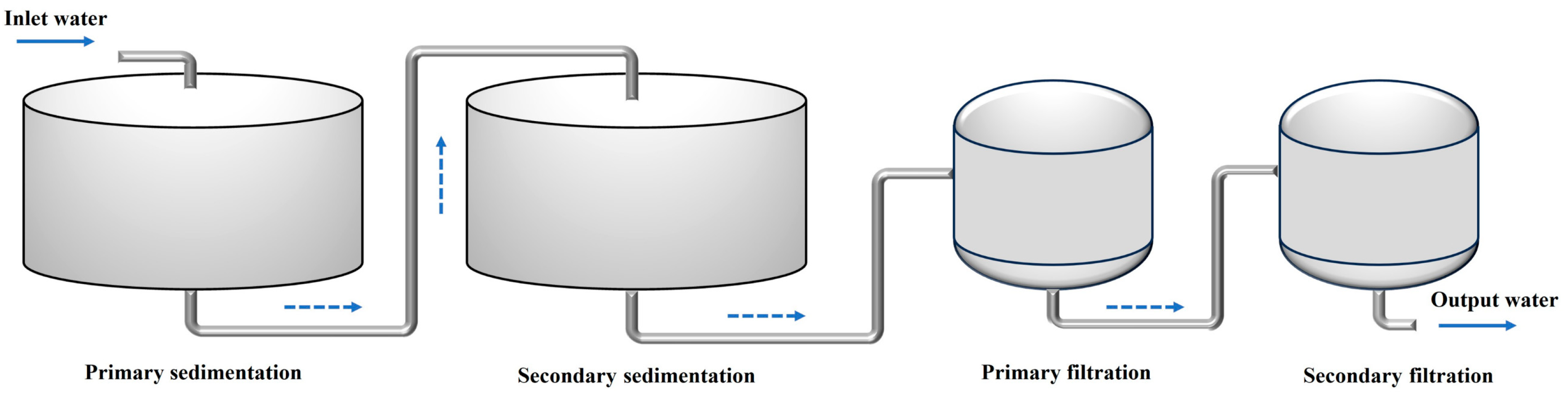
2. Production Description

Oilfield produced water is generally categorized into three types based on the composition and concentration of chemical agents: water flooding, polymer flooding, and ASP flooding. Based on polymer concentration, polymer-flooding produced water can be classified into three categories: low concentration (<150 mg/L), normal concentration (150–450 mg/L), and high concentration (>450 mg/L) [32,33]. In oilfield production, the produced water treatment processes of water flooding and low polymer concentration are similar. The produced water is filtered by walnut shell filter material after two-stage sedimentation treatment. The processes of two-stage sedimentation and one-stage filtration is adopted for common and high polymer concentration produced water. The difference is that quartz sand filter material is used for common polymer concentration produced water, while quartz sand and magnetite double filter material are used for high polymer concentration produced water. The alkali, surfactant, and chemical components in ASP flooding produced water complicate its treatment process. Oilfield employs a treatment process comprising dual sedimentation stages followed by dual filtration stages, utilizing quartz sand and magnetite as filter material. Figure 1 shows the full process flow. The output water from secondary sedimentation flows into the filtration tank, where filter material provides dual mechanisms of interception and adsorption to achieve additional removal of oil and suspended solids [34,35]. The generally accepted treatment standard limit for produced water specifies that both oil content and suspended solids content should be below 20 mg/L [33].

3. Methodology

3.1. Basic Parameters

This research involved sampling and testing ASP flooding produced water from an oilfield in eastern China. Samples were taken from the inlet of the produced water treatment station. The polymer concentrations in the produced water samples were analyzed. Basic parameters, including interfacial tension (35 °C, oil–water), oil/suspended solids content in produced water, and their respective size distributions, were also measured to establish a basis for further investigation [36,37,38,39]. Based on the measurement of oil and suspended solids content, the produced water from ASP flooding can be classified into three classes.

Table 1. The basic parameters of ASP flooding produced water.

Classification	Oil Droplets Average Size, μm	Suspended Solids Average Size, μm	Polymer Concentration, mg/L	Oil Content, mg/L	Suspended Solids Content, mg/L	Interfacial Tension, mN/m
class I	0.742	16.53	358.7	538.0	532.0	0.154
class II	0.767	17.04	276.0	303.0	297.0
class III	0.689	15.09	415.2	138.0	145.0

presents its basic parameters.

3.2. Model Construction

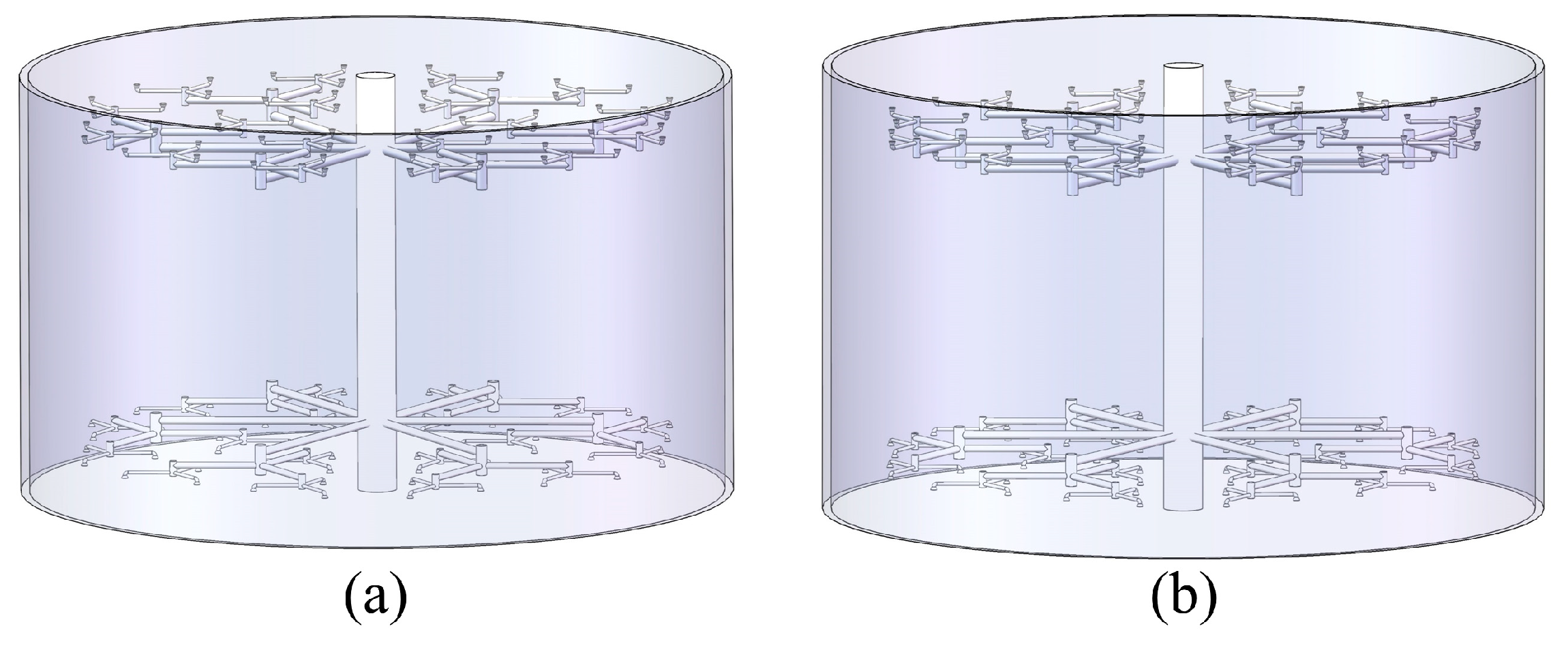
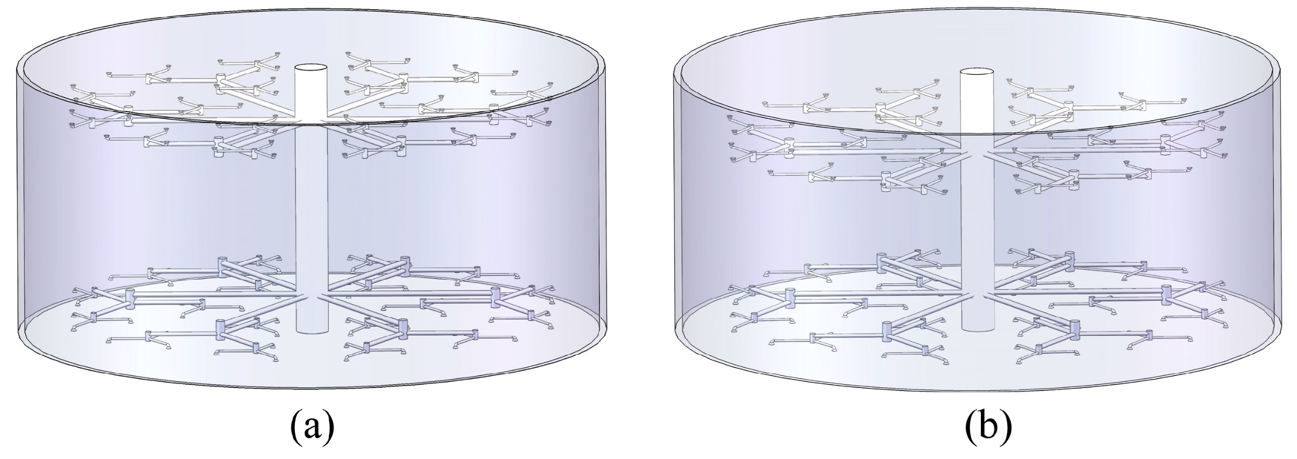
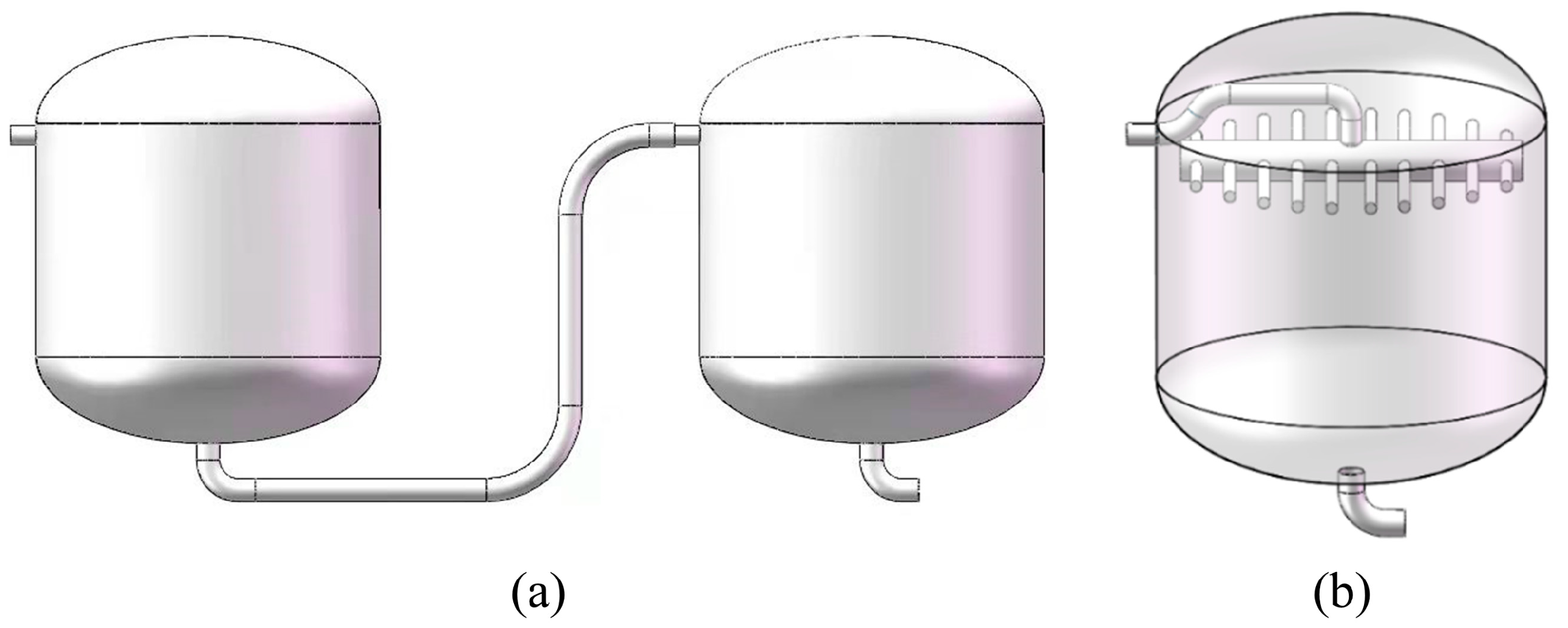
3.2.1. Physical Models

The numerical simulation of the treatment process of class I, class II, and class III ASP flooding produced water was carried out. For the convenience of subsequent discussion, the treatment processes of the three classification ASP flooding produced water were called class I, class II, and class III, respectively.

Table 2. Structural dimensions of sedimentation tanks.

Classification of Treatment Process	Structural Dimensions of Primary Sedimentation Tank	Structural Dimensions of Secondary Sedimentation Tank
class I	Φ32,500 mm × 12,000 mm	Φ32,500 mm × 12,000 mm
class II	Φ16,300 mm × 12,700 mm	Φ16,300 mm × 12,700 mm
class III	Φ27,200 mm × 12,800 mm	Φ27,200 mm × 12,800 mm

presents the structural dimensions of sedimentation tank models designed for various classes of ASP flooding produced water treatment.

For class I, II, and III treatment processes, the corresponding simplified physical models of sedimentation tanks are shown in Figure 2, Figure 3 and Figure 4.

Unlike sedimentation, the ASP flooding produced water treatment process employs filtration tanks of identical size, using the same filter material and grading ratio. Figure 5 displays the physical model of the filtration tank. Both primary and secondary filtration are filled with quartz sand and magnetite double filter material. The quartz sand filter material layer has a thickness of 500 mm, while the magnetite filter material layer is 300 mm thick.

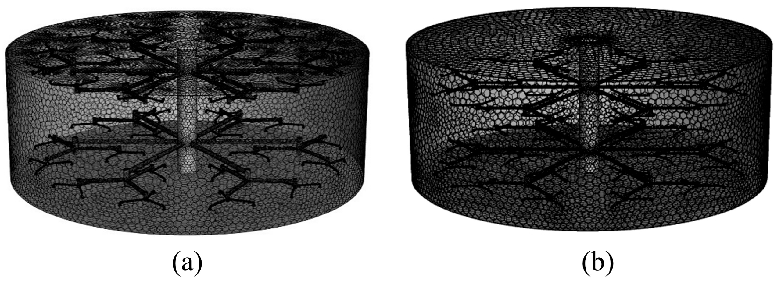
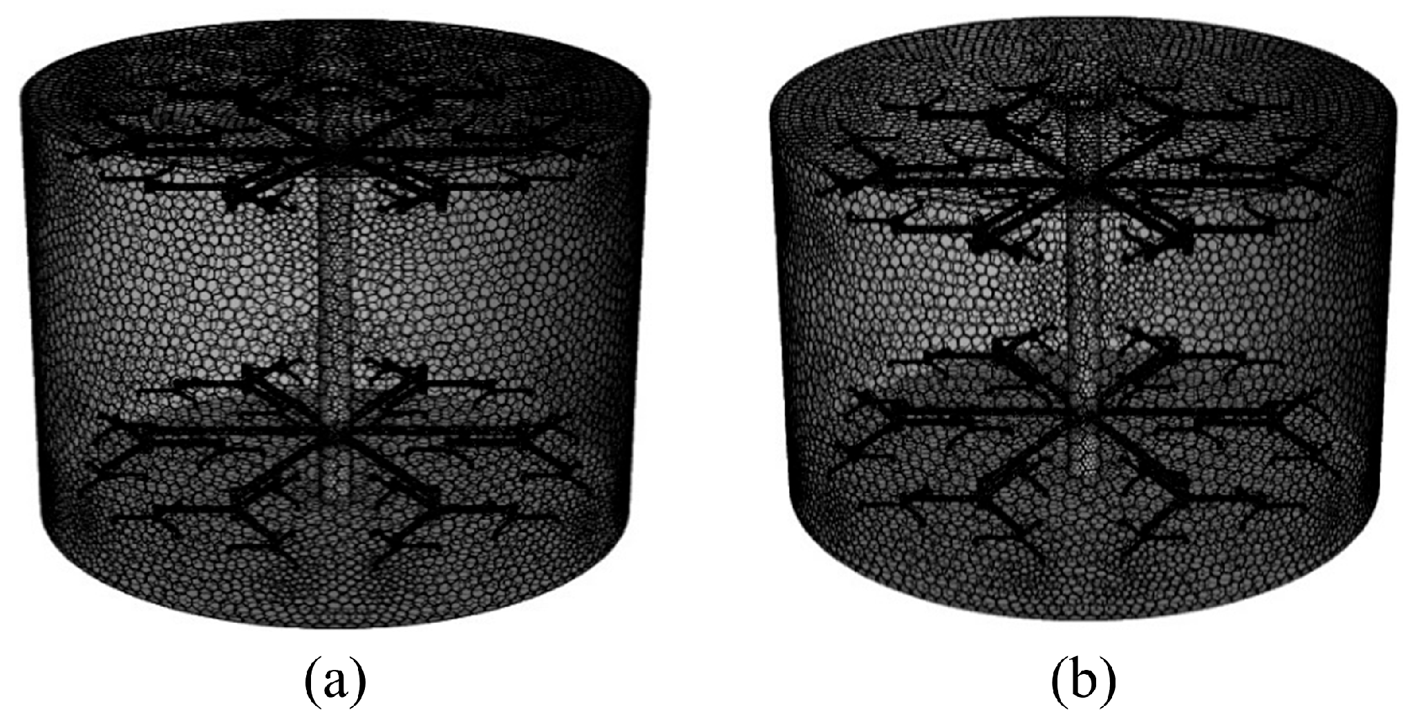
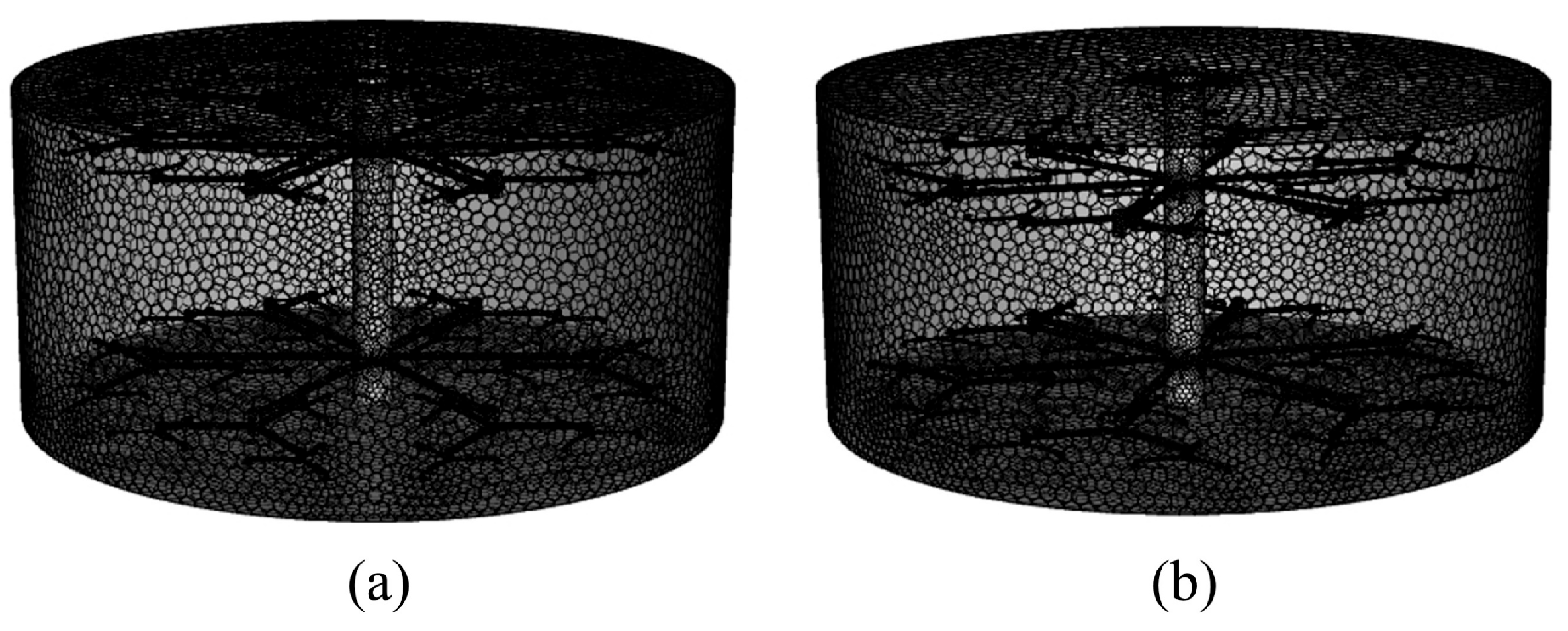
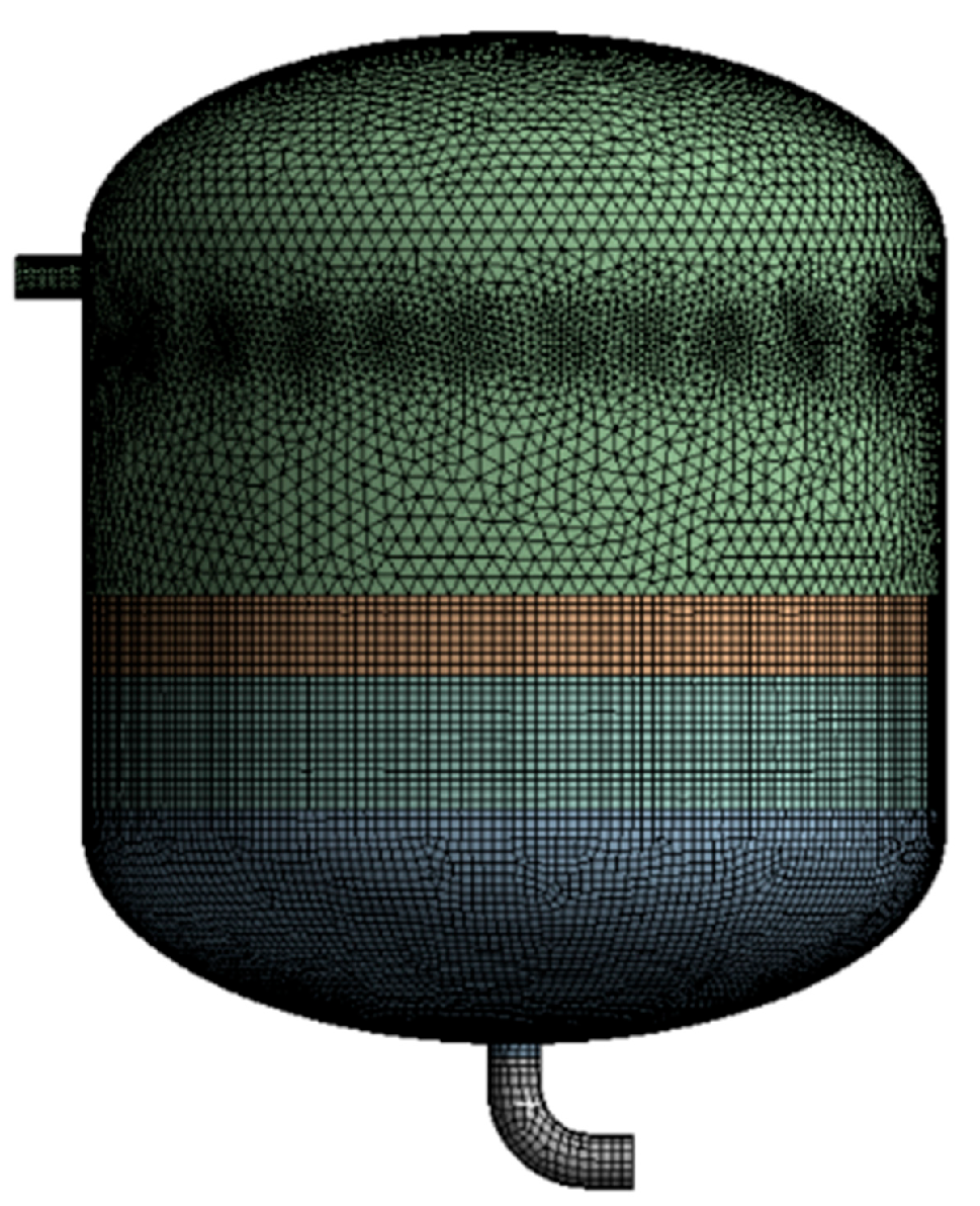
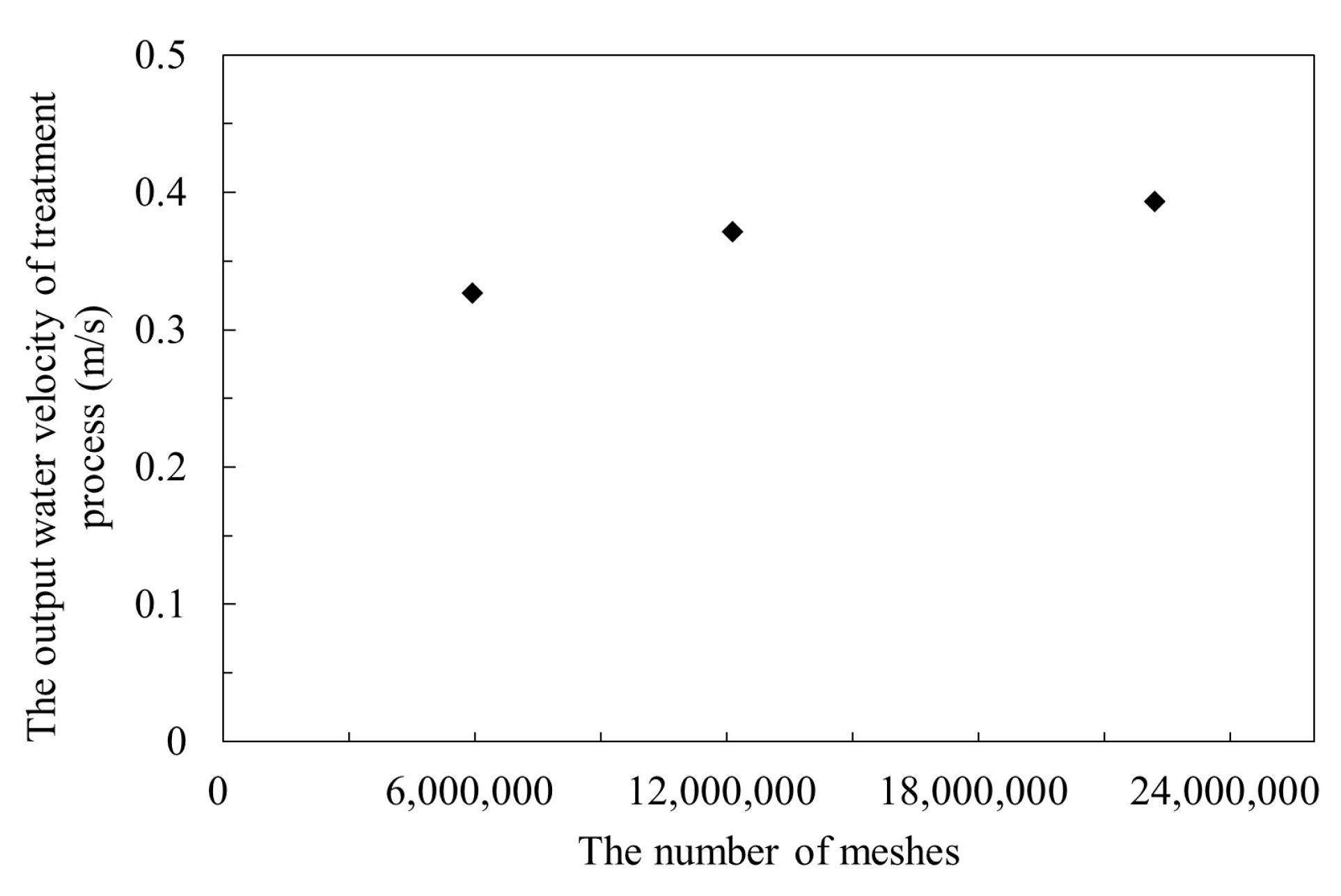
3.2.2. Mesh Generation and Independence Validation

The physical models of the sedimentation tank and the filtration tank were meshed. Figure 6, Figure 7, Figure 8 and Figure 9 display the meshing results. Mesh independence verification was conducted using the physical model of class I produced water treatment process. The inlet water contained 0.08% oil and 0.02% suspended solids, with a treatment amount of 13,600 m³/d and an inlet pressure of 2 MPa. Mesh independence was verified by comparing the output water velocities from simulations using sparse, normal, and refined meshes.

3.2.3. Mathematical Models

Regarding the gravity sedimentation process, the Eulerian approach was employed because all mixture components could be treated as continuous phases. In this study, the RNG k–ε turbulence model was selected to simulate the flow field [18].

The continuity equation is as follows:

$${\displaystyle \frac{\partial }{\partial t}}({\rho }_m)+\nabla ·({\rho }_m{\overrightarrow{v}}_m)=0$$

(1)

The momentum equation is as follows:

$${\displaystyle \frac{\partial }{\partial t}}({\rho }_m{\overrightarrow{v}}_m)+\nabla ·({\rho }_m{\overrightarrow{v}}_m{\overrightarrow{v}}_m)=-\nabla p+\nabla ·\left[{\mu }_m\left(\nabla {\overrightarrow{v}}_m+\nabla {{\overrightarrow{v}}_m}^T\right)\right]+{\rho }_{m}g+\overrightarrow{F}+\nabla ·({\displaystyle \sum _{k=1}^n{\sigma }_k{\rho }_k{\overrightarrow{v}}_{dr,k}}{\overrightarrow{v}}_{dr,k})$$

(2)

$${\overrightarrow{v}}_m={\displaystyle \frac{{\displaystyle \sum _{k=1}^n{\alpha }_k{\rho }_k}{\overrightarrow{v}}_k}{{\rho }_m}}$$

(3)

$${\overrightarrow{v}}_{dr,k}={\overrightarrow{v}}_k-{\overrightarrow{v}}_m$$

(4)

The turbulence model is as below:

$${\displaystyle \frac{\partial }{\partial t}}(\rho k)+{\displaystyle \frac{\partial }{\partial x_i}}(\rho k{u}_i)={\displaystyle \frac{\partial }{\partial x_j}}\left[{\alpha }_k{\mu }_{eff}{\displaystyle \frac{\partial k}{\partial x_j}}\right]+G_k+G_b+S_k-\rho \epsilon -Y_M$$

(5)

$${\displaystyle \frac{\partial }{\partial t}}(\rho \epsilon )+{\displaystyle \frac{\partial }{\partial x_i}}(\rho \epsilon u_i)={\displaystyle \frac{\partial }{\partial x_j}}\left[{\alpha }_{\epsilon }{\mu }_{eff}{\displaystyle \frac{\partial \epsilon }{\partial x_j}}\right]+C_{1\epsilon }{\displaystyle \frac{\epsilon }{k}}(G_k+C_{3\epsilon }{G}_b)+S_{\epsilon }-C_{2\epsilon }\rho {\displaystyle \frac{{\epsilon }^2}{k}}-R_{\epsilon }$$

(6)

$G_k$ and $G_b$ can be obtained from Equations (7) and (8), respectively.

$$G_k=\left({\displaystyle \frac{\partial u_i}{\partial x_j}}+{\displaystyle \frac{\partial u_j}{\partial x_i}}\right){\displaystyle \frac{\partial u_i}{\partial x_j}}{\mu }_t$$

(7)

$$G_b=-{\displaystyle \frac{1}{\rho }}{\displaystyle \frac{\partial \rho }{\partial T}}{g}_i{\displaystyle \frac{{\mu }_i}{p_{r_t}}}{\displaystyle \frac{\partial T}{\partial x_i}}$$

(8)

$${\mu }_t=\rho C_{\mu }{\displaystyle \frac{k^2}{\epsilon }}$$

(9)

where $C_{\mu }$ = 0.0845.

The porous medium model is introduced for filtration numerical simulation, and the momentum source is calculated based on Equation (10) [40,41].

$$S_u=(-{\displaystyle \frac{\mu }{\alpha }}v)+(-C{\displaystyle \frac{1}{2}}\rho |v|v)$$

(10)

where $\mu$ is the hydrodynamic viscosity coefficient, Pa·s; $\rho$ is the fluid density, kg/m³; ${\displaystyle \frac{1}{\alpha }}$ is the viscous resistance coefficient, 1/m²; $C$ is the inertial drag coefficient, 1/m; ${\displaystyle \frac{1}{\alpha }}$ and $C$ can be calculated by Equations (11) and (12), respectively.

$${\displaystyle \frac{1}{\alpha }}={\displaystyle \frac{150{(1-\epsilon )}^2}{D_p^2{\epsilon }^3}}$$

(11)

$$C={\displaystyle \frac{3.5(1-\epsilon )}{D_p{\epsilon }^3}}$$

(12)

where $D_p$ is the particle diameter, m; $\epsilon$ is the porosity.

3.3. Solution Model

3.3.1. Simulate Conditions and Parameters

According to the operational data of the ASP flooding produced water treatment process, scatterplots of treatment amount distribution and output water quality distribution of each treatment process are drawn. The numerical simulation parameters are determined based on the distribution intervals of treatment capacity and treated water quality.

According to the operation data of class I treatment process, the scatterplot of treatment amount distribution and output water quality distribution of each treatment process is drawn. Scatterplots are shown in Figure 10. The maximum and minimum treatment amounts are 16,000 m³/d and 13,600 m³/d, respectively, and the oil and suspended solids content in the output water is significantly higher than 20 mg/L. Add a median of 14,800 m³/d between the maximum and minimum treatment amount as the numerical simulation condition.

The scatterplot in Figure 11 shows the class II treatment amount distribution and output water quality distribution. The treatment amount is distributed between 8000 m³/d and 11,600 m³/d, and the oil and suspended solids content in the output water is significantly higher than 20 mg/L. Based on the extreme value distribution of treatment amount, 4400 m³/d is selected as the numerical simulation condition.

For class III treatment process, Figure 12 illustrates the correlation between treatment amount and output water quality. The maximum and minimum treatment amounts are 14,000 m³/d and 9200 m³/d, respectively, and the output water fails to meet the standard limit of 20 mg/L for both oil and suspended solids content. Add a median of 11,600 m³/d between the maximum and minimum treatment amount as the numerical simulation condition.

Based on the above analysis, numerical simulations were conducted with the treatment amount and inlet water polymer concentration as independent variables. Different numerical simulation conditions were established to investigate the treatment capacity of ASP flooding produced water under varying operational conditions. The simulation scheme is presented in

Table 3. Simulation scheme of treatment capacity for ASP flooding produced water treatment.

Classification of Treatment Process	Treatment Amount, m3/d	Inlet Water Polymer Concentration, mg/L
class I	13,600/14,800/16,000	300/400/500
class II	4400/8000/11,600	200/300/400
class III	9200/11,600/14,000	300/400/500

.

Treatment amount is an important parameter affecting the produced water treatment process of ASP flooding. Therefore, when the polymer concentration of inlet water is constant, the output water quality characteristics under different treatment amounts are explored for a certain content range of oil and suspended solids. Operation limits for the ASP flooding produced water treatment process are established to ensure that the treated water meets oil and suspended solids specifications of 20 mg/L, with the simulation methodology detailed in

Table 4. Simulation scheme of operation limits for ASP flooding produced water treatment.

Classification of Treatment Process	Treatment Amount, m3/d	Inlet Water Oil Content, mg/L	Inlet Water Suspended Solids Content of, mg/L
class I	13,600/14,800/16,000	100/300/500	100/300/500
class II	4400/8000/11,600	100/200/300	100/200/300
class III	9200/11,600/14,000	50/100/150	50/100/150

.

3.3.2. Model Assumptions and Limitations

This study is based on the oilfield site and makes some assumptions to simplify the numerical simulation and improve the solution efficiency. The produced water is assumed to be an incompressible isothermal fluid, and the structure of oil droplets and suspended solids is a regular sphere. The following assumptions are made about the simulation conditions in the filtration process: suspended particles in the inlet water are evenly distributed, and the distribution of the inlet water is uniform. The filter material particles in the filter material layer are regarded as isotropic.

The temperature of produced water in oilfields generally fluctuates slightly within a certain range, and the temperature has an impact on the viscosity of the produced water. In this study, the median of the temperature fluctuation range (35 °C) was selected as the numerical simulation temperature to minimize the influence of temperature fluctuation on the treatment effect.

For the main parameters that affect filtration, such as porosity, viscous resistance coefficient, and inertial resistance coefficient, the simulated parameters are consistent with the actual model. The shapes of quartz sand and magnetite filter materials used in the filtration of produced water from ASP flooding are close to a uniform spherical shape. Therefore, it is assumed that the filter material is isotropic, and the differences in physical properties and arrangement methods of the filter material in different directions are ignored. The influence of this assumption on the simulation results is acceptable.

In the process of oilfield produced water treatment, there may be chemical interactions among oil droplets, suspended solids, and polymers. The polymer forms an adsorption layer on the surface of oil droplets and particles, hindering the collision and aggregation of oil droplets and suspended solids, which affects the treatment effect of the produced water. Ignoring these chemical reactions will make the simulation processing effect slightly better than the actual field. The viscous resistance coefficient and inertial drag coefficient of porous media corresponding to different filter materials are shown in

Table 5. Filter simulation parameters.

Filter Material Type	Particle Size Distribution of Filter Material, mm	Average Particle Size of Filter Material, mm	Viscous Resistance Coefficient, 108 m−2	Inertial Drag Coefficient, 104 m−1
Quartz sand filter material of primary filtration	0.8~1.2	0.8	9.5776	3.1365
Magnetite filter material of primary filtration	0.4~0.8	0.6	11.2732	2.9778
Quartz sand filter material of secondary filtration	0.5~0.8	0.6	17.0268	4.1820
Magnetite filter material of secondary filtration	0.25~0.5	0.4	25.3647	4.4667

.

3.3.3. Solution Methods

The sedimentation process is simulated by a transient with a time step ranging from 0.1 s to 4 s, which is dynamically adjusted according to the size of the simulation residual. The numerical model of sedimentation separation uses a velocity inlet boundary for the inflow and a pressure outlet boundary for the outflow. The simulation adopts the Phase Coupled SIMPLE algorithm, with the gradient discretization term evaluated through Least-Squares cell-based interpolation. The pressure discrete term is selected as Second Order, the momentum discrete term is First Order Upwind, and the time discrete term is First Order Implicit.

The filtration process is simulated by a transient with a time step of 2 s. The filtration simulation utilizes a velocity inlet boundary condition for the inflow and a pressure outlet boundary condition for the outflow. For the DPM model, considering the influence of drag force and virtual mass force, there are random collisions between particles. The particle size distribution of suspended particulates is a Rosin-Rammler distribution. The pressure–velocity coupling adopts the SIMPLE algorithm, with the gradient discretization term being Least-Squares cell-based, and the pressure discrete term being Body Force Weighted.

3.3.4. Data Extraction and Processing

The phase volume fraction distributions are obtained through cross-sectional analyses at multiple locations within the sedimentation tank physical model, facilitating analysis of oil phase and suspended solids concentration variations. Equation (13) calculates the oil/suspended solids removal rate in the sedimentation tank.

$$\phi ={\displaystyle \frac{V_{inlet}-V_{outlet}}{V_{inlet}}}\times 100\%$$

(13)

where $\phi$ is the removal rate, %; $V_{inlet}$ is the inlet water oil/suspended solids content, mg/L; $V_{outlet}$ is the output water oil/suspended solids content, mg/L.

To calculate the filtration removal rate, a sampling plane is established at the bottom boundary of the filter material layer, and the oil droplets and suspended solids passing through the plane during the filtration process are counted. The quantitative assessment of filtration effectiveness is accomplished by computing the oil droplets and suspended solids removal rate according to Equation (14).

$$n_f={\displaystyle \frac{{10}^{-6}\cdot n_0\cdot c-\rho {\displaystyle \sum _{i=1}^n{V}_{fi}}}{{10}^{-6}\cdot n_0\cdot c}}\times 100\%$$

(14)

where $n_f$ is the oil droplets/suspended solids removal rate, %; $n_0$ is the concentration of oil droplets/suspended solids in the inlet water, mg/L; $c$ is the amount of filtered water, L; $V_{fi}$ is the volume of oil droplets/suspended solids passing through the sampling plane during the filtration process, m³; $i$ is the number of oil droplets/suspended solids passing through the sampling plane during the filtration process; $\rho$ is the oil/suspended solid density, kg/m³.

3.4. Model Validation

Eight sets of daily operational data were selected from the class III ASP flooding produced water treatment process, as detailed in

Table 6. Daily production data of produced water treatment process.

Serial Number	Treatment Amount, m3/d	Oil Content, mg/L	Suspended Solids Content, mg/L
1	13,554	146.2	153.6
2	13,782	135.7	140.9
3	13,888	139.5	146.4
4	12,590	143.7	155.9
5	13,246	132.6	146.5
6	14,403	134.3	144.3
7	12,159	145.5	147.7
8	13,692	141.3	143.4

. Taking the data in Table 6 as the numerical simulation parameters, the water treatment process of class III produced water was simulated, and the water quality parameters after treatment were extracted. The simulation results were compared with the real-world production data to verify the accuracy of the simulation models.

4. Results and Discussion

4.1. Result of Independence Validation

As illustrated in Figure 13, the mesh-independence validation demonstrates a solution error of 11.92% between sparse and normal meshes. And the discrepancy between normal and refined meshes diminishes to 5.71%, falling below the 10% tolerance limit. The normal meshes provide an optimal balance between accuracy and efficiency, making them the preferred choice for numerical simulations.

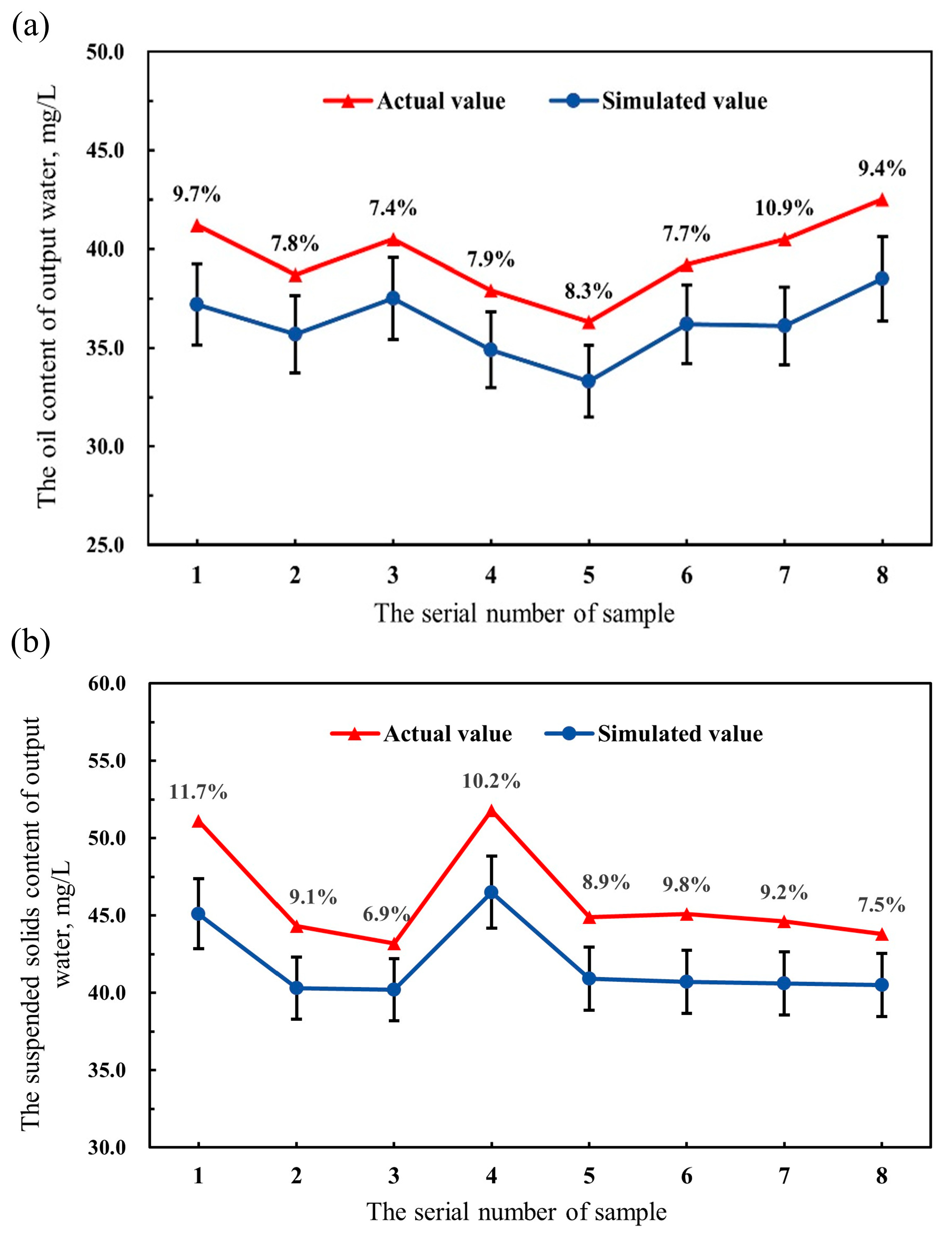
4.2. Result of Model Validation

The comparison between simulated values and actual values is shown in Figure 14. It can be seen that the error range of the oil content is 7.4~10.9%, and the average error is 8.6%. The error range of suspended solids content is 6.9~10.2%, with an average error of 9.1%. Under different operating conditions, the variation trend of simulated output water quality parameters is consistent with the real-world parameters. Moreover, the oil and suspended solids content in the simulation results is lower than that in the actual results. This is because the oil collection of the sedimentation tank and the backwashing of the filter material are not timely in the field production, which affects the water quality and makes it worse than the simulation results. This confirms that the numerical simulation results are in line with the real world, and the predicted operating limits are accurate.

4.3. Sedimentation Operation Characteristics

According to the numerical simulation conditions in Table 3, the sedimentation process of class I, class II, and class III ASP flooding produced water treatment processes was simulated. Corresponding to each operating condition, the oil phase and suspended solids volume fraction distributions were extracted and subjected to quantitative evaluation.

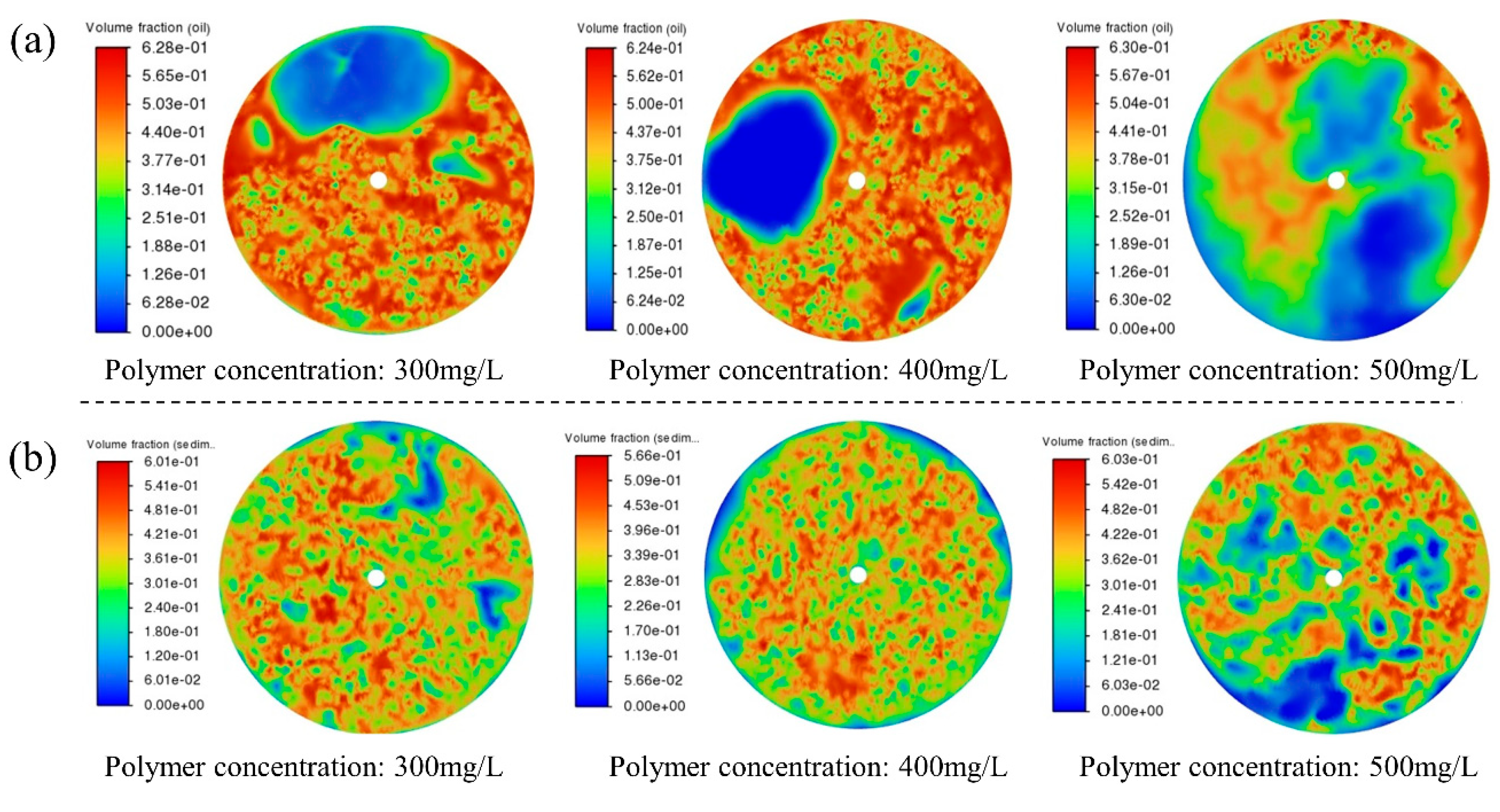
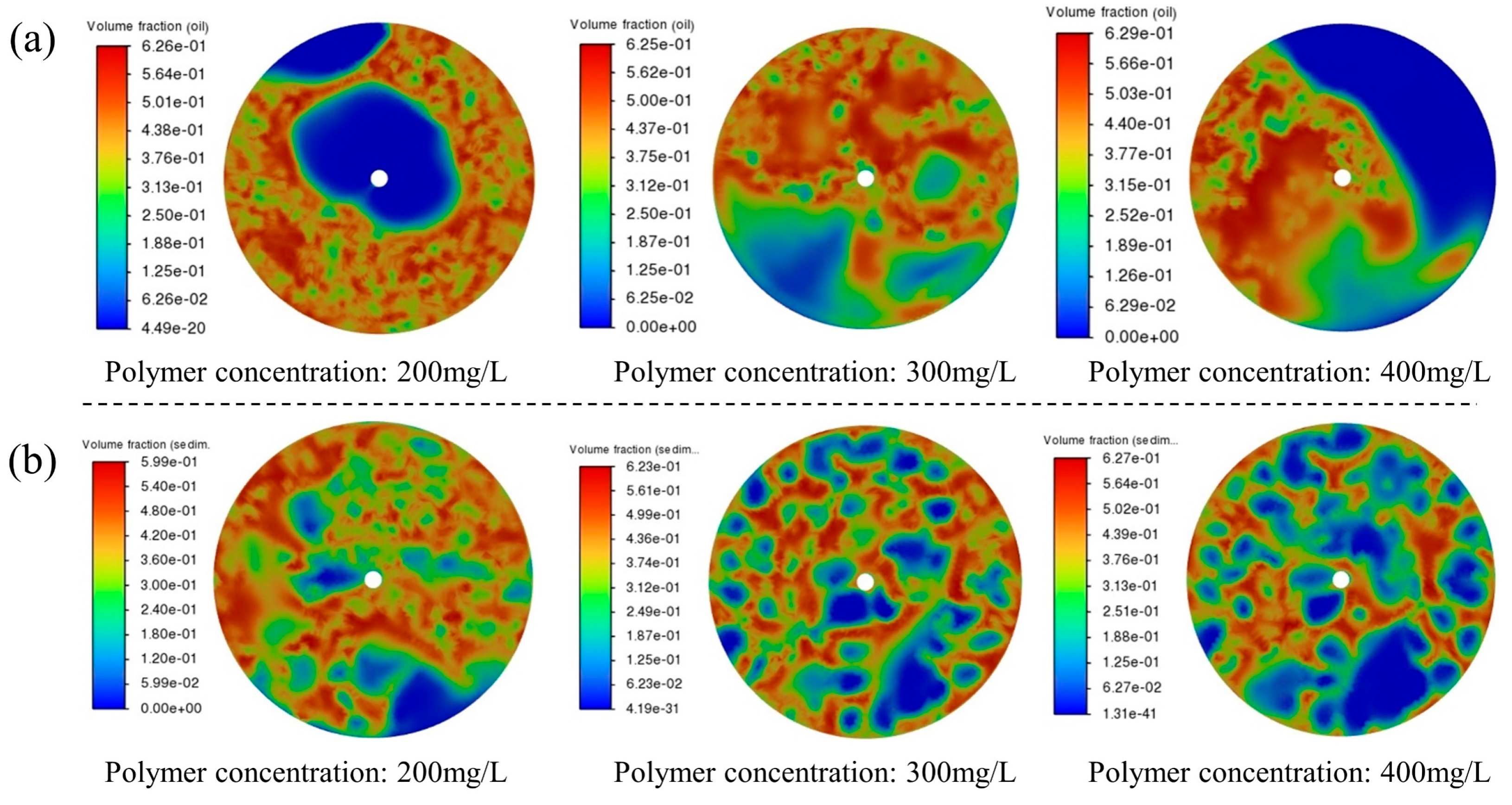
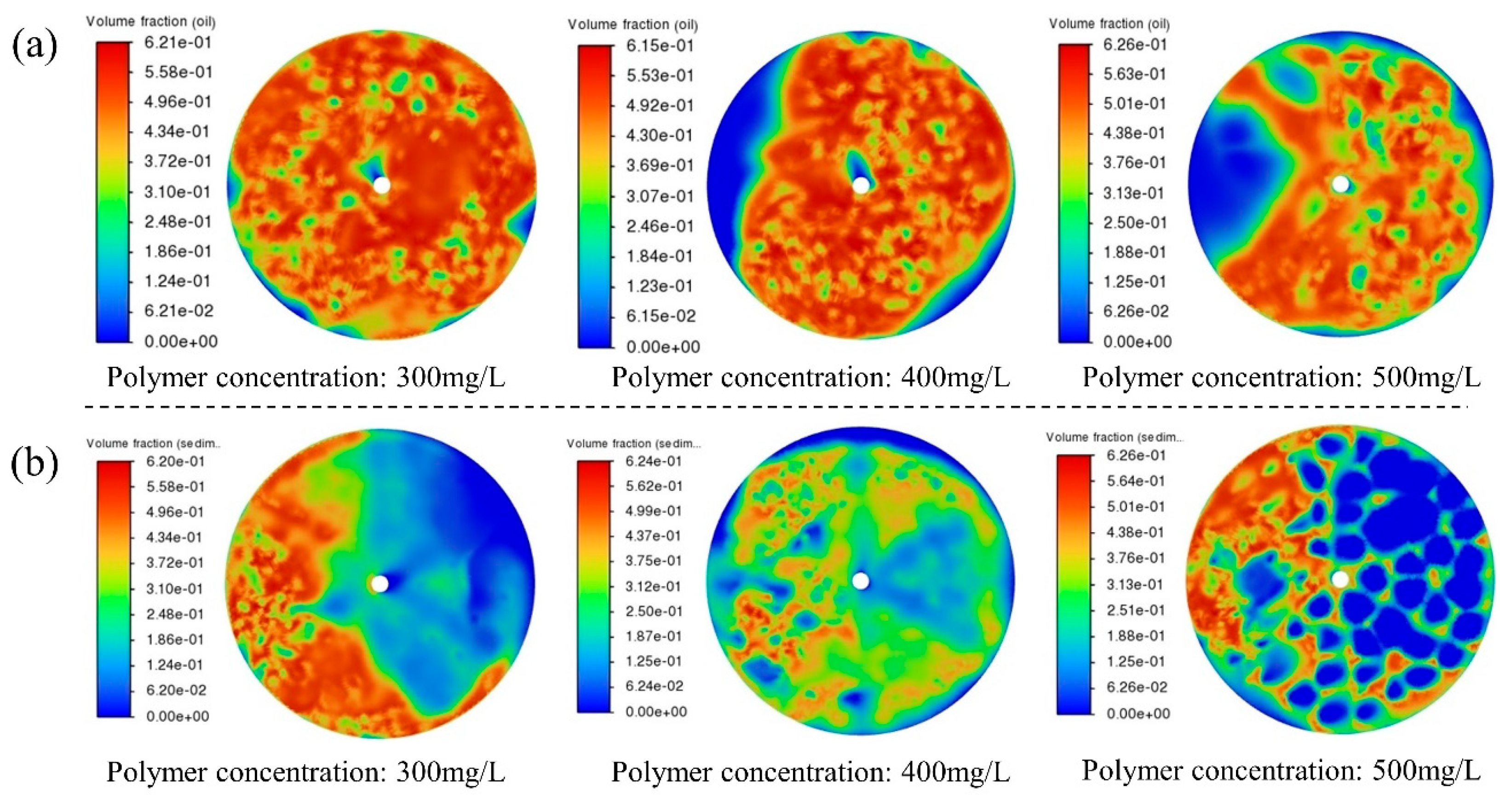
4.3.1. Primary Sedimentation

The oil phase and suspended solids volume fraction distributions were characterized using cross sections positioned 10 mm below the upper surface and 3 mm above the lower surface of the sedimentation tank fluid domain. For the class I treatment process, the oil phase and suspended solids distribution at the treatment amount of 14,800 m³/d are shown in Figure 15. Combined with the distribution characteristics of the treatment amount of 13,600 m³/d and 16,000 m³/d, the following results are obtained. In the oil phase distribution, high-concentration zones predominantly form clustered sheets, and low-concentration zones display dense point patterns. Under identical treatment amounts, the area of high oil phase concentration in the cross section diminishes as the inlet water’s polymer concentration increases. Under consistent inlet water concentration, the oil phase boundary between high and low concentration areas blurred as the treatment amount increases, showing a progressive homogenization of the concentration field. The suspended solids display a discontinuous, scattered arrangement in high-concentration areas, while the low-concentration area shows a continuous distribution. Under the same treatment amount, the suspended solids concentration in the cross section decreases with the increase in inlet water polymer concentration, and the area of the low concentration area increases. For inlet water with the same concentration of polymer, as the treatment amount increases, the distinction between high and low suspended solids concentration areas becomes progressively less defined.

For the class II treatment process operating at 8000 m³/d, distribution characteristics are illustrated in Figure 16. Combined with the distribution characteristics of the treatment amount of 4400 m³/d and 11,600 m³/d, the following results are obtained. Increasing the inlet water’s polymer concentration reduces the high-concentration oil phase area, whereas at fixed polymer concentrations, a greater treatment amount leads to a lower oil phase concentration in the cross section. Similar to the oil phase behavior, higher polymer concentrations in inlet water lead to both decreased high-concentration areas and progressive dispersion of suspended solids into low-concentration zones.

For the class III treatment process operating at 11,600 m³/d, distribution characteristics are illustrated in Figure 17. Combined with the distribution characteristics of the treatment amounts of 9200 m³/d and 14,000 m³/d, the following results are obtained. Under identical treatment amounts, higher polymer concentrations in inlet water lead to a gradual decrease in high-concentration zones for both the oil phase and suspended solids. The boundary between areas of high and low oil phase concentration is less defined as the concentration distribution evens out, whereas the area with high suspended solids concentration migrates toward the tank wall. At fixed polymer concentration in the influent, higher treatment volumes lead to decreased oil and suspended solids concentrations, along with diminished high-concentration regions.

During primary sedimentation, the content of oil and suspended solids is measured in both the inlet and output water. The removal rates are calculated using Equation (13), and the change characteristics of the removal rate in the primary sedimentation process are obtained, as shown in Figure 18. During primary sedimentation, the oil removal efficiency is higher than that of suspended solids under the same operating conditions. Under constant polymer concentration in produced water, the removal efficiency exhibits an inverse relationship with treatment volume. Conversely, at constant treatment amount, higher polymer concentration reduces both oil and suspended solids removal efficiency.

4.3.2. Secondary Sedimentation

The oil phase and suspended solids volume fraction distributions were characterized using cross sections positioned 5 mm below the upper surface and 2 mm above the lower surface of the sedimentation tank fluid domain. For the class I treatment process operating at 14,800 m³/d, the oil phase and suspended solids distribution patterns in the secondary sedimentation are illustrated in Figure 19. Comparative analysis of distribution characteristics was conducted at flow rates of 13,600 m³/d and 16,000 m³/d, with results presented below. The oil phase exhibits concentrated distribution patterns in high-concentration zones and discrete point distribution in low concentration areas. With the increase in polymer concentration of inlet water, both the oil phase concentration and oil phase area in the cross section decrease, while for the same polymer concentration of inlet water, as the treatment amount increases, the oil phase concentration decreases. Suspended solids display a homogeneous distribution pattern, differing from the oil phase, with point-like distribution in high-concentration areas. Under the same treatment amount, as the polymer concentration of the inlet water increases, the high-concentration zones of suspended solids decrease. The volume distribution and variation characteristics of class II and III treatment processes exhibit fundamental consistency with those observed in class I.

The variation characteristics of the removal rate in secondary sedimentation are presented in Figure 20. The secondary sedimentation process demonstrates lower removal rates for both oil phase and suspended solids compared to primary sedimentation, while exhibiting similar variation patterns. However, compared to the primary sedimentation, the influence of polymer concentration on removal efficiency is more significant in the secondary sedimentation.

4.4. Filtration Operation Characteristics

The filtration process of class I, II, and III treatment processes was simulated. After the stable operation of filtration, the distribution characteristics of oil droplets and suspended solids in the filtration process were extracted. And the influence of operating conditions (treatment amount, polymer concentration) on the filtration removal rate was qualitatively analyzed.

4.4.1. Primary Filtration

For the class I treatment process, oil droplets and suspended solids distribution characteristics at the treatment amount of 14,800 m³/d are shown in Figure 21. The following analysis compares oil droplets and suspended solids distribution patterns between treatment amounts of 13,600 m³/d and 16,000 m³/d. In the area above the filter material layer, the oil droplets and suspended solids are in a free state. The filter material layer exhibits a graded particle size distribution: the upper section is dominated by larger droplets of oil and suspended solids, while the deeper layers primarily contain smaller particles. The upper filter material layer shows increased free oil droplets and suspended solids at elevated polymer concentration, with oil droplets representing the larger proportion. This is because oil droplets are less dense and float more easily than suspended solids. Furthermore, elevated polymer concentrations in the influent increase particle breakthrough in the filter material layer due to competitive adsorption between polymers, oil droplets, and suspended solids on filter media surfaces, which reduces overall adsorption efficiency. When the polymer concentration of inlet water remains unchanged, higher treatment amount leads to more and larger particles escaping below the filter media layer, and the majority are suspended solids. This indicates that the increase in the treatment amount can also degrade the performance of the filter material. In both class II and class III treatment processes, oil droplets and suspended solids exhibit distribution and variation patterns similar to the class I process.

The removal efficiency trends for oil droplets and suspended solids in the primary treatment are illustrated in Figure 22. Primary filtration typically removes oil droplets more effectively than suspended solids. At stable polymer concentrations, higher processing volumes resulted in decreased removal performance for both oil and suspended solids contaminants. Similarly, at a fixed treatment amount, higher polymer concentrations in the inlet water resulted in lower removal efficiencies for both contaminants.

4.4.2. Secondary Filtration

Different from the primary filtration, the secondary filtration uses finer filter material particles. For the class I treatment process, the distribution characteristics at the treatment amount of 14,800 m³/d are shown in Figure 23. In the secondary filtration process, the distribution characteristics of suspended particles are similar to those in the primary filtration. However, at the same depth of the filter material layer, the particle size of the suspended particles further decreases. Smaller filter particles increase the material’s specific surface area, thereby expanding the water-contact interface and enhancing the filter layer’s adsorption capacity for fine suspended particles. And for secondary filtration of the class II and class III treatment process, the distribution and variation characteristics of oil droplets and suspended solids are consistent with the class I treatment process.

Figure 24 displays the removal rate characteristics in secondary filtration, as calculated by Equation (14) for oil droplets and suspended solids under various working conditions.

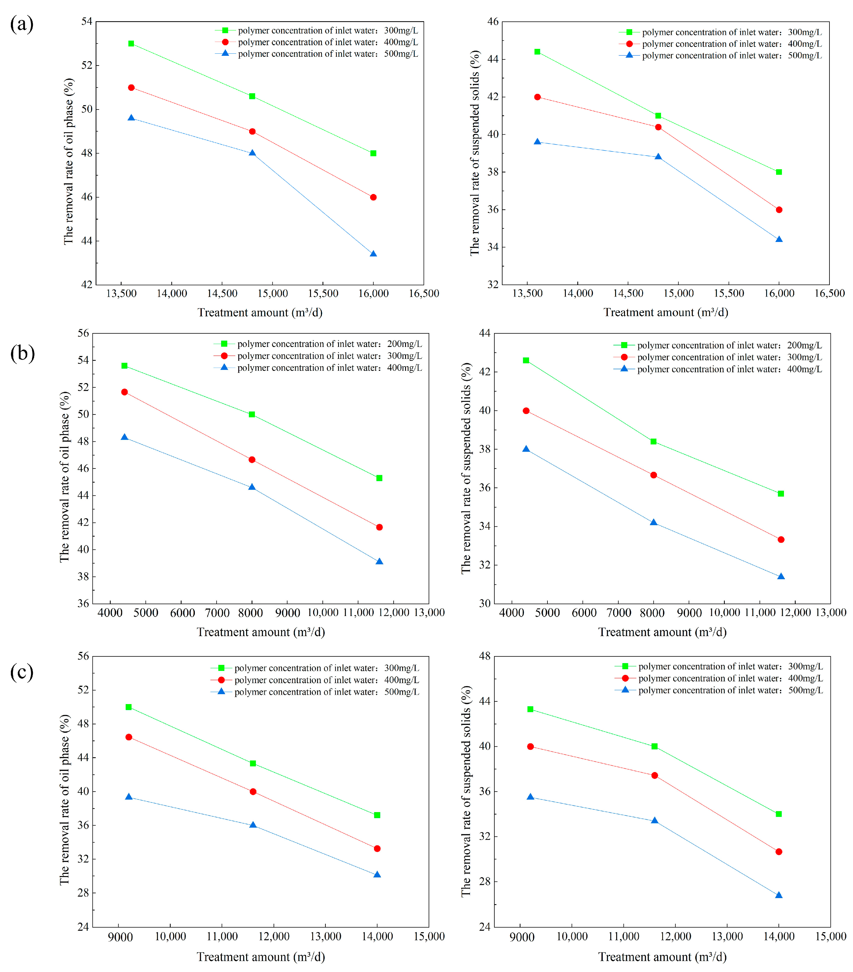
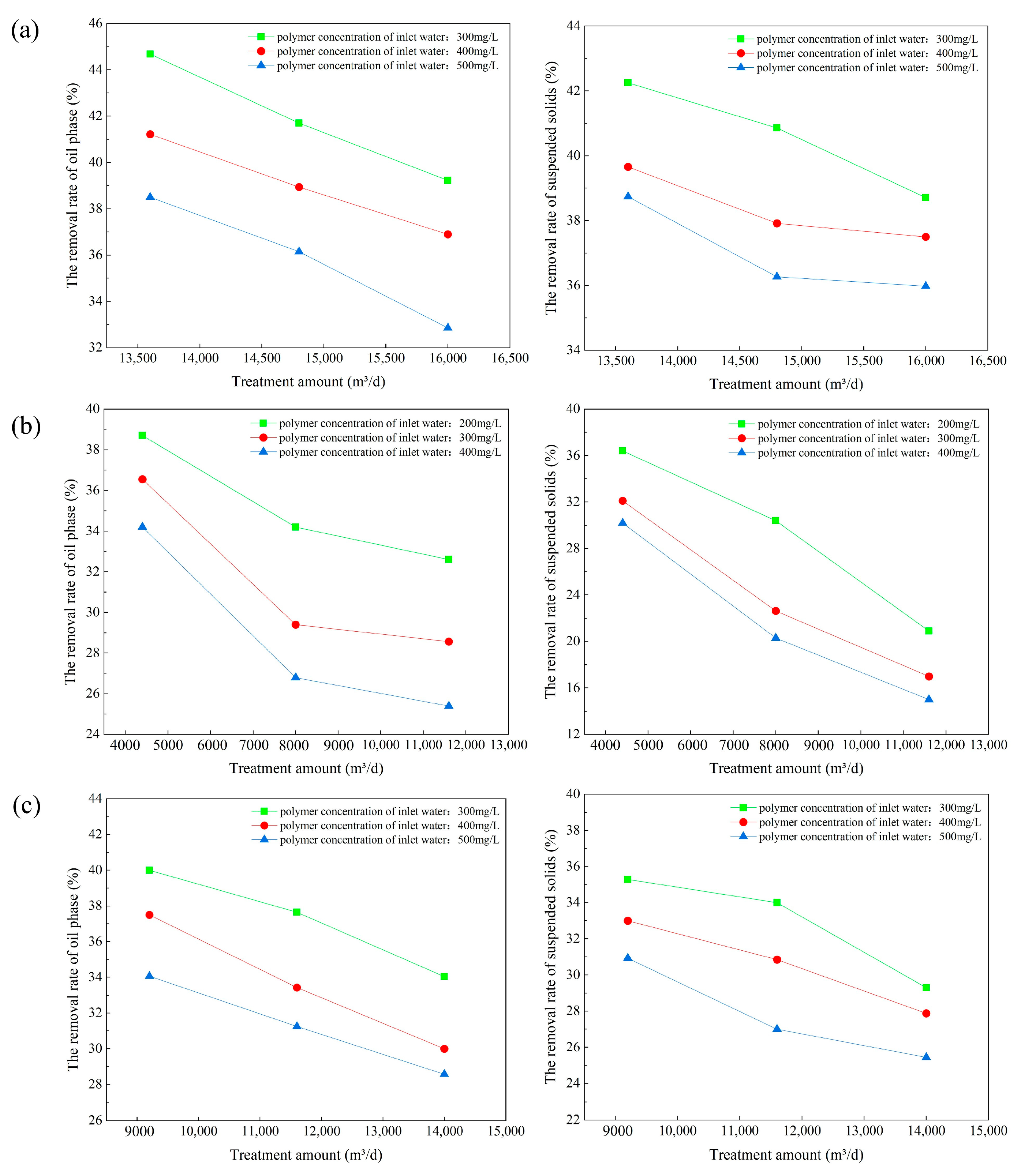
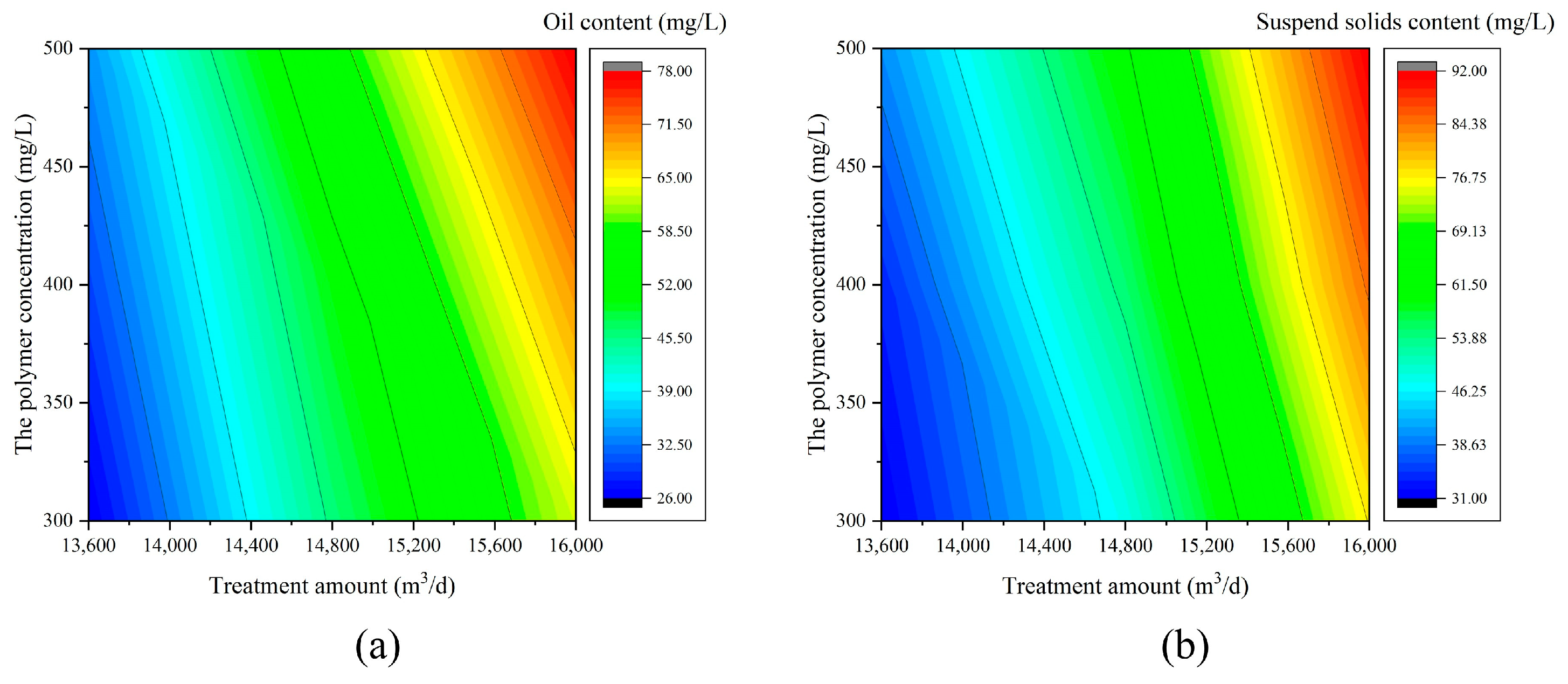
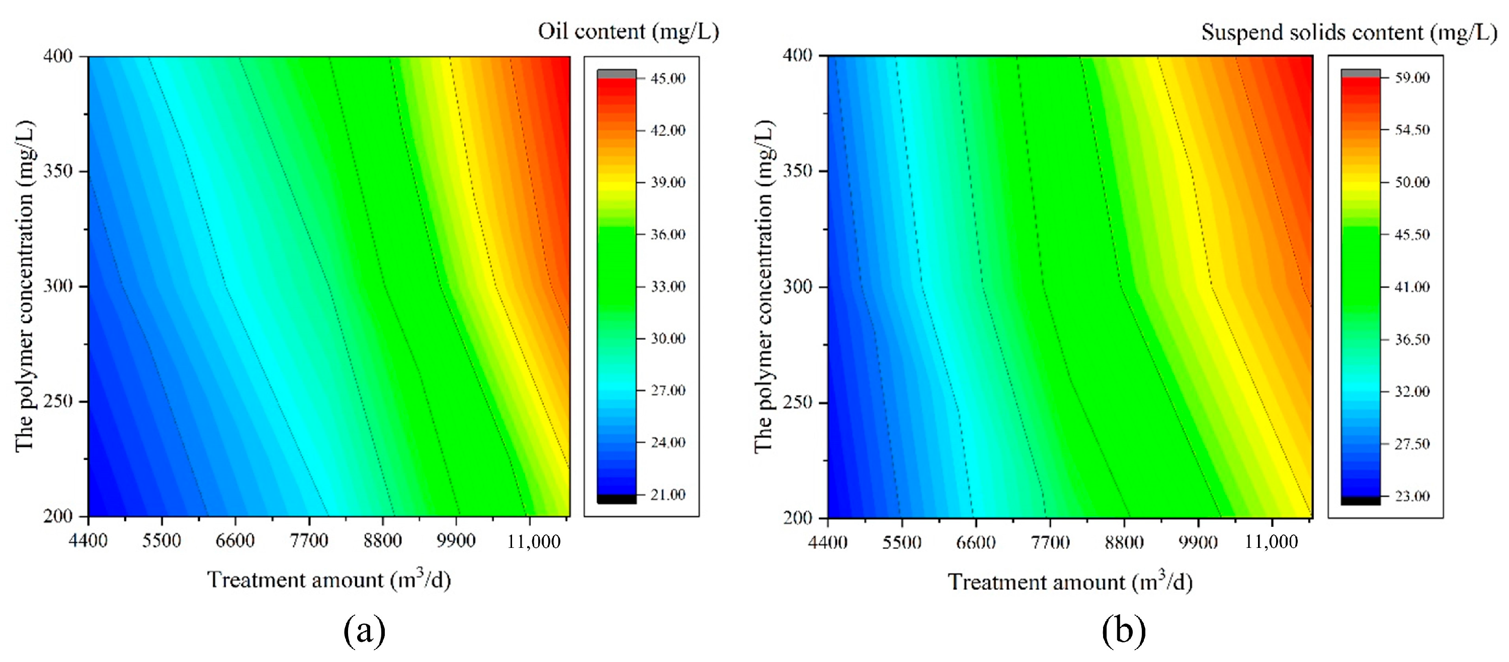
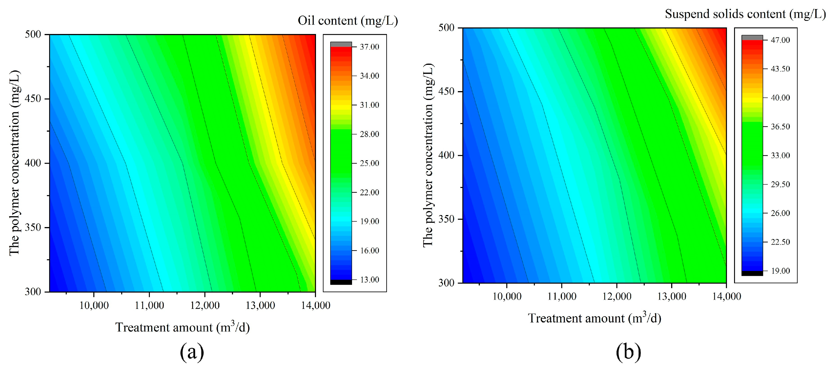
4.5. Treatment Capacity of Treatment Process

The oil and suspended solids content in the secondary filtered water are extracted during numerical simulation. Established the distribution pattern of water quality and studied the treatment capacity of the treatment process. Figure 25 presents the oil and suspended solids content in the output water from the class I treatment process. The oil content ranges from 26 to 78 mg/L, while suspended solids range from 31 to 92 mg/L, both exceeding the 20 mg/L treatment standard limit for water quality. Figure 26 presents the oil and suspended solids content distributions in the class II treatment process treated water. The treated water contains oil concentrations of 21–45 mg/L and suspended solids ranging from 23 to 59 mg/L, which do not meet the treatment standard limit. Figure 27 presents the treated produced water quality from the class III process, showing distributions of both oil content and suspended solids. The oil content varies between 13 and 37 mg/L, and the suspended solids content ranges from 19 to 47 mg/L, which meets the treatment standard limit under some working conditions. Under the influence of polymer, alkali, and surfactant, the oil droplets in ASP flooding produced water exhibit smaller sizes and severe emulsification. In addition, the chord length of suspended solids is also reduced. Due to its elevated polymer content and viscosity, ASP flooding produced water exhibits a strong capacity to carry suspended particles, which severely diminishes the treatment capacity of sedimentation and filtration processes.

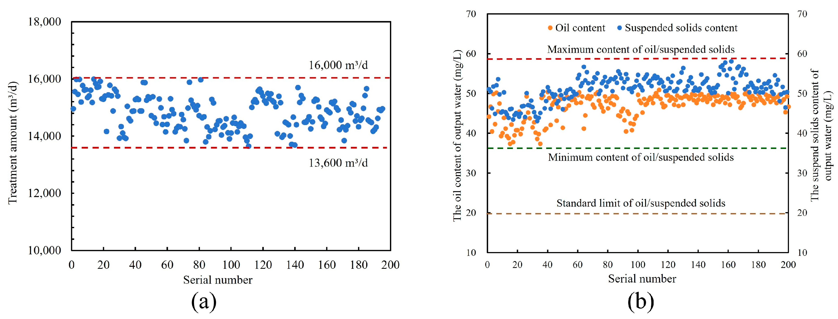
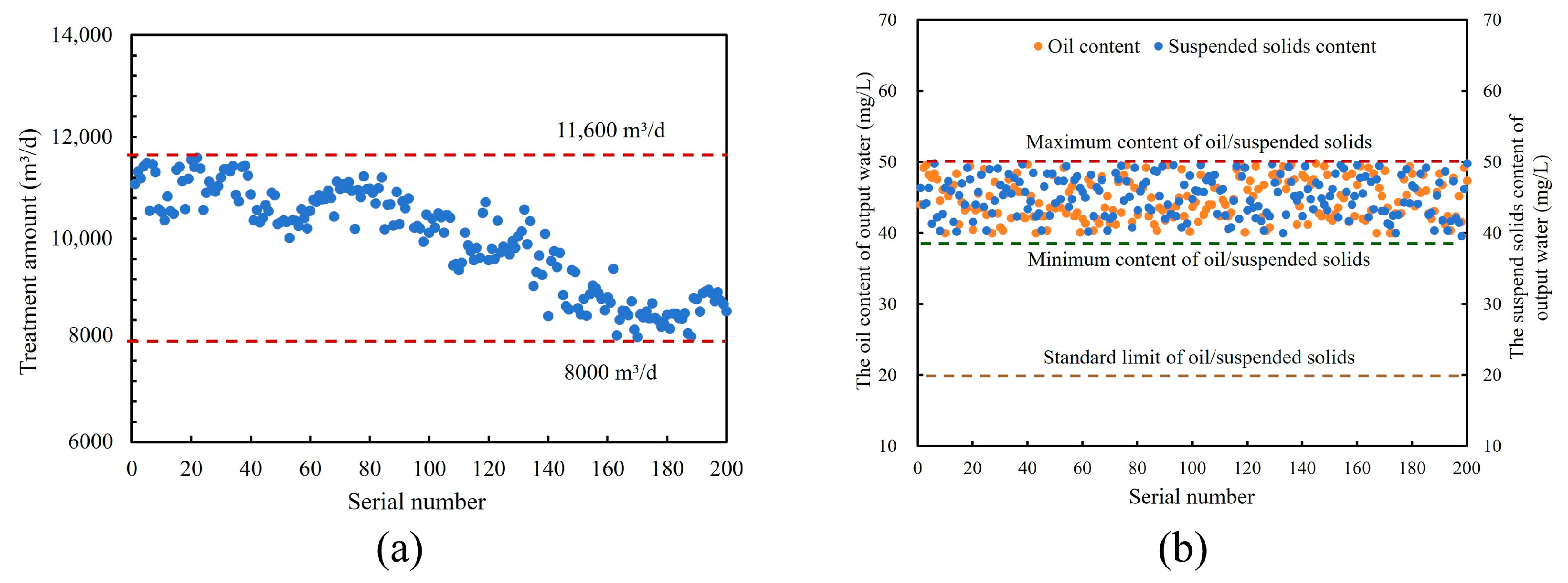
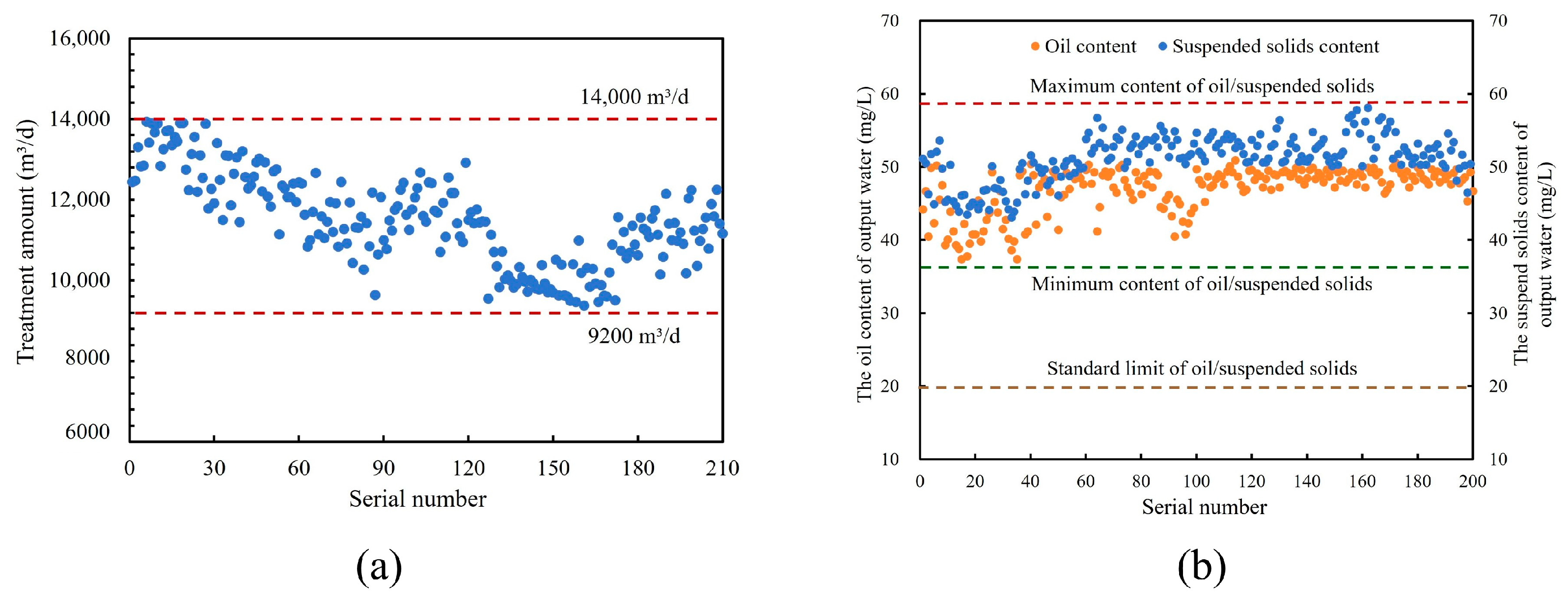
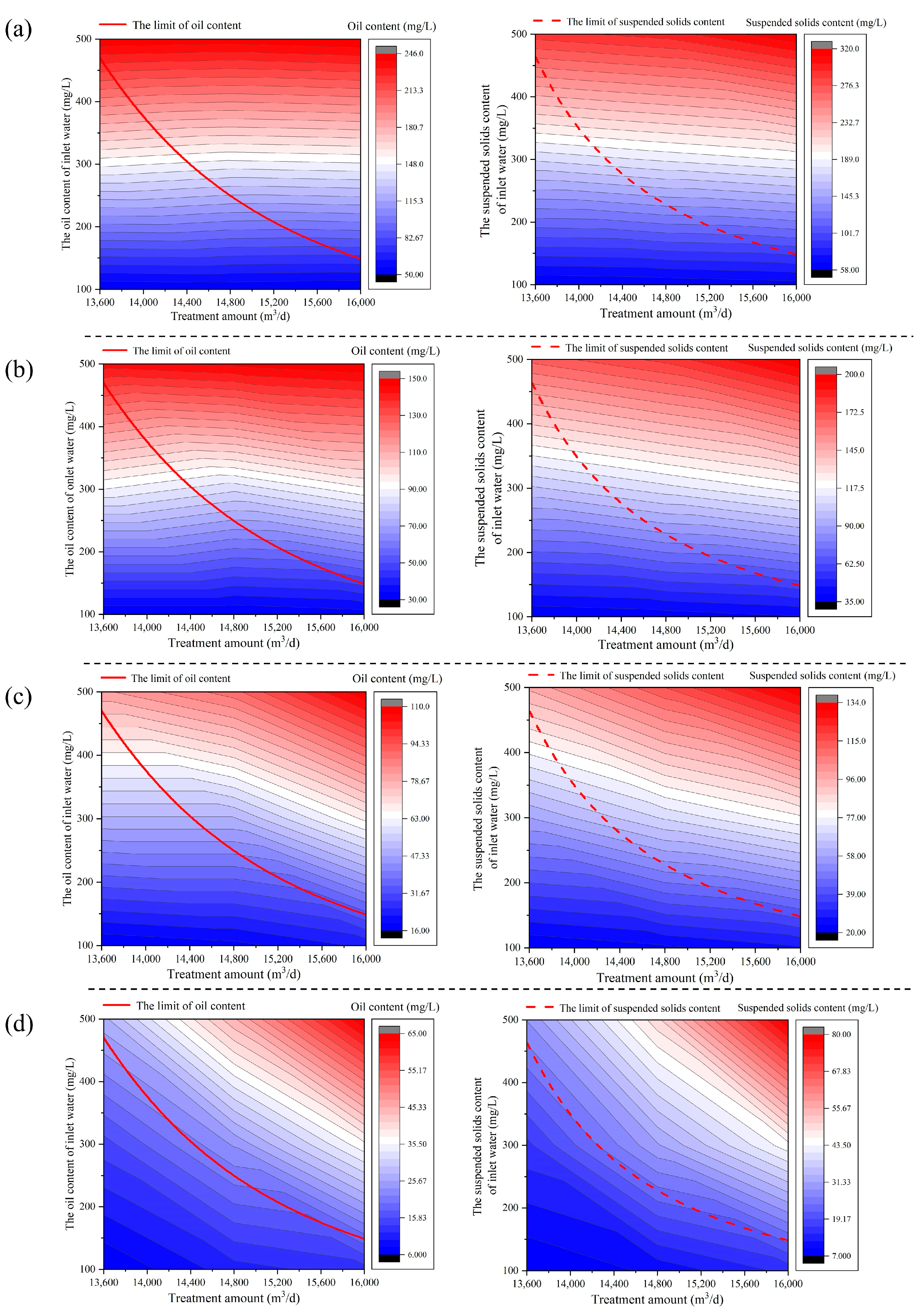
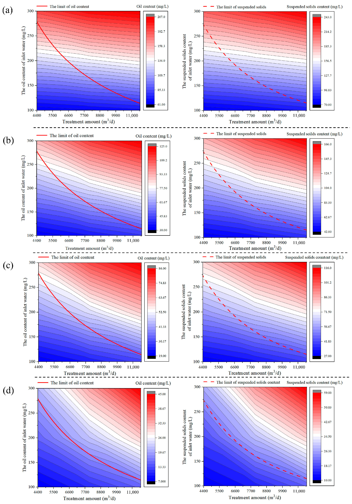
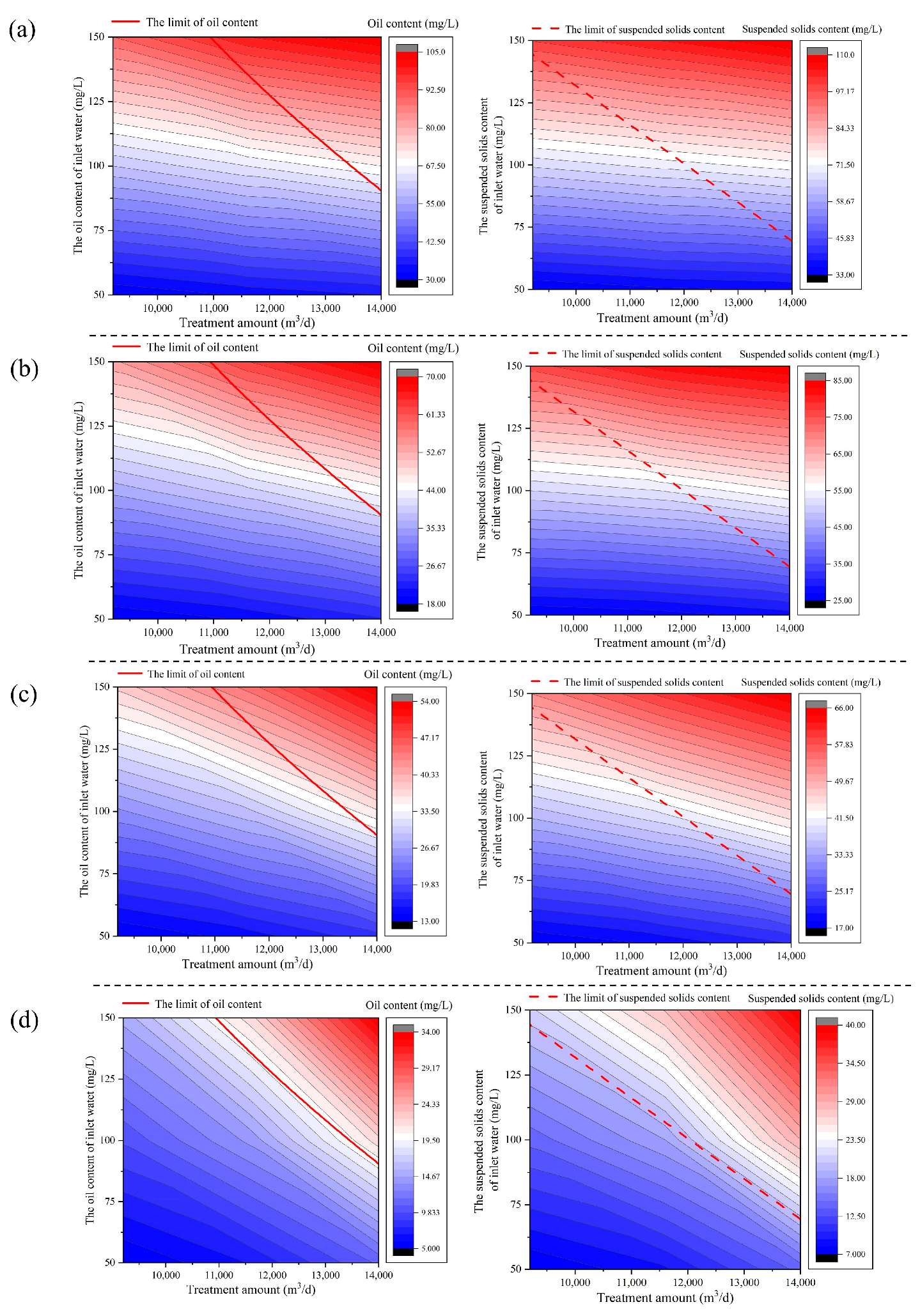
4.6. Operating Limits of Treatment Process

The produced water treatment process for ASP flooding was simulated using the conditions specified in Table 4. The oil and suspended solids content of produced water from four treatment nodes of primary sedimentation outlet, secondary sedimentation outlet, primary filtration outlet, and secondary filtration outlet were extracted, respectively.

4.6.1. Operating Limits of Class I Treatment Process

Based on the numerical simulation results, a polynomial fitting method was employed to establish the relationship between treatment amount, inlet water oil content, and output water oil content. Similarly, a correlation is established among the treatment amount, inlet water suspended solids content, and output water suspended solids content. Equation (15) is the fitting relation between treatment amount ($x$), inlet water oil content ($y$), and output water oil content ($f_o\left(x,y\right)$), and the fitting degree R² is 0.9808. Equation (16) is the fitting relation between treatment amount ($x$), inlet water suspended solids content ($y$), and output water suspended solids content ($f_s\left(x,y\right)$), and the fitting degree R² is 0.9968.

$$\begin{array}{l}{f}_o\left(x,y\right)=9.861-0.0003819x-0.4263y\\ +3.229\times {10}^{-5}xy+6.25\times {10}^{-5}{y}^2\end{array}$$

(15)

$$\begin{array}{l}{f}_s\left(x,y\right)=19.53-0.001215x-0.5746y\\ +4.47\times {10}^{-5}xy+2.917\times {10}^{-5}{y}^2\end{array}$$

(16)

Based on the polynomial fitting results of Equations (15) and (16), the polynomial interpolation method is used to find the operating conditions when the oil and suspended solids content in the output water are 20 mg/L. The oil content limit curves are drawn in the oil content distribution maps of the output water from each treatment node, and the limit curves of suspended solids are the same, as shown in Figure 28.

The area at the lower-left of the limit curves represents the operating conditions where the water quality treatment meets the standards, whereas the upper-right area represents the conditions where the water quality treatment fails to meet the standards. When the operating conditions meet the left area of the oil and suspended solids content limit curve, it indicates that the output water of the class I treatment process is qualified under this condition, and the corresponding limits are the operating limits.

4.6.2. Operating Limits of Class II Treatment Process

Fit the binomial functions of oil content and suspended solids content in the output water of the class II treatment process separately, as shown in Equations (17) and (18), and the fitting degree R² are 0.9996 and 0.9983, respectively.

$$\begin{array}{l}{f}_o\left(x,y\right)=0.0823-0.0002521x+0.03444y+1.286\times {10}^{-8}{x}^2\\ +1.111\times {10}^{-5}xy-3.333\times {10}^{-5}{y}^2\end{array}$$

(17)

$$\begin{array}{l}{f}_s\left(x,y\right)=-0.01646+0.0003189x+0.01611y-2.572\times {10}^{-8}{x}^2\\ +1.528\times {10}^{-5}xy+1.667\times {10}^{-5}{y}^2\end{array}$$

(18)

The polynomial interpolation function is used to establish the operating limits of class II treatment process under variable operating conditions, as shown in Figure 29. In the treatment amount range of 4400–11,600 m³/d, when the oil and suspended solids content are in the range of 100–275 mg/L, and the operating conditions are below the limit curves, the output water meets the standards.

4.6.3. Operating Limits of Class III Treatment Process

Equations (19) and (20) are binomial functions of oil content and suspended solids content in the output water of class III treatment process, and the fitting degree R² are 0.9987 and 0.9971, respectively.

$$\begin{array}{l}{f}_o\left(x,y\right)=43.88-0.007523x-0.1808y+3.183\times {10}^{-7}{x}^2\\ +2.708\times {10}^{-5}xy-0.0001333y^2\end{array}$$

(19)

$$\begin{array}{l}{f}_s\left(x,y\right)=51.38-0.009722x-0.05333y+4.34\times {10}^{-7}{x}^2\\ +2.5\times {10}^{-5}xy-0.0002y^2\end{array}$$

(20)

The polynomial interpolation function is used to establish the operating limits of class III treatment process under variable operating conditions, as shown in Figure 30. When the treatment amount is within the range of 9000–14,000 m³/d, with oil content of 50–150 mg/L and suspended solids content of 50–144 mg/L, the treated water meets standards as long as the operating conditions are below the limit curves.

5. Conclusions

Numerical simulations were conducted to analyze oil and suspended solids distributions under different operating conditions in ASP flooding produced water treatment. By analyzing the influence of operating conditions on the treatment capacity, the treatment capacity and operation limits of the ASP flooding produced water treatment process were obtained. The specific conclusions are as follows:

(1)

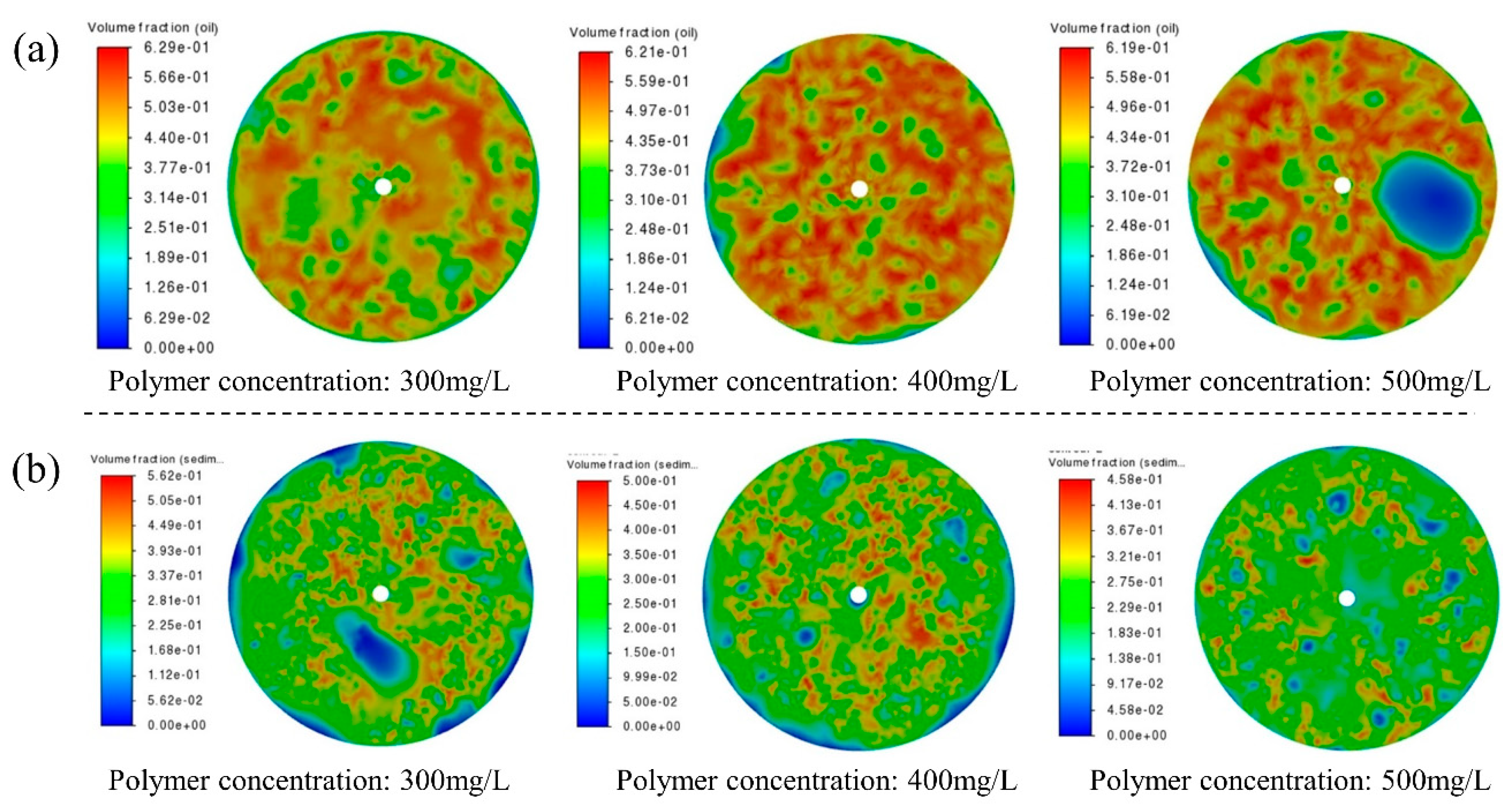
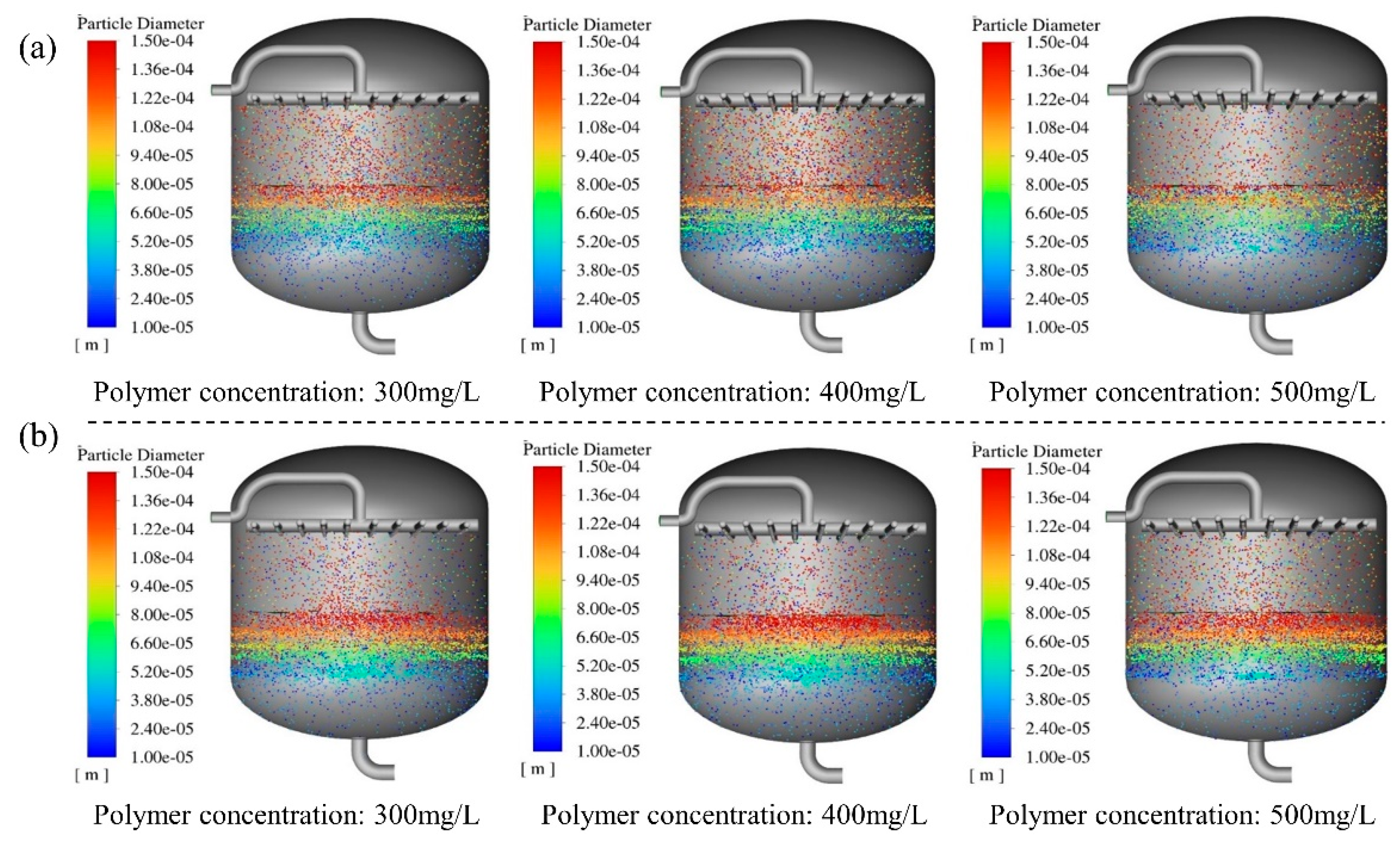
For produced water treatment, elevated treatment volumes and increased polymer concentrations in the influent water adversely affect both sedimentation separation efficiency and filter media adsorption capacity. More specifically, the concentrations of both oil and suspended solids in the sedimentation tank exhibit significant reductions, accompanied by a corresponding diminishment of high-concentration zones within the respective oil and suspended solids layers. Concurrently, the filtration process shows an increase in the number of escaping particles under the filter material.

(2)

The simulation results show that the oil content range of treated water from the class I treatment process is 26–78 mg/L, and the suspended solid content is 31–92 mg/L. The output water oil content of the class II treatment process is 21–45 mg/L, and the suspended solid content is 23–59 mg/L. The oil content of the output water from class III treatment process is 13–37 mg/L, and the suspended solid is 19–47 mg/L. Under certain operating conditions, the treated water meets the standards with both oil and suspended solids content below 20 mg/L.

(3)

Based on the numerical simulation results, the polynomial interpolation method was employed to determine the water quality parameters for each treatment node, ensuring that the treated produced water meets the standard with oil and suspended solids content below 20 mg/L. The operating limits of the ASP flooding produced water treatment process are established. Take the class II treatment process as an example. Within the treatment amount range of 4400–11,600 m³/d, the treated water meets quality standards when the oil and suspended solids content of the produced water is between 100 and 275 mg/L, and operating conditions stay below the limit curves.

References

1. Ji, B.; Xu, T.; Gao, X.; Yu, H.; Liu, H. Production evolution patterns and development stage division of waterflooding oilfields. Pet. Explor. Dev. 2023, 50, 433–441. [Google Scholar] [CrossRef]
2. Chang, S.; Wang, M.; Wang, M. The identification of the development stages of the karstic fracture-cavity carbonate reservoirs: A case study on the lungu oilfield, Tarim basin. Front. Earth Sci. 2023, 11, 1238759. [Google Scholar] [CrossRef]
3. Hu, G.; Tian, X.H.; Liu, Q.W.; Yi, L.Z.; Liu, D.W.; Li, P.C. Quick assessment to ascertain technical rational well spacing density in artificial water flooding oilfield. J. Pet. Sci. Eng. 2021, 196, 108087. [Google Scholar] [CrossRef]
4. Wang, Y.W.; Liu, H.Q.; Zhang, Q.C.; Chen, Z.X.; Wang, J.; Dong, X.H.; Chen, F.X. Pore-scale experimental study on EOR mechanisms of combining thermal and chemical flooding in heavy oil reservoirs. J. Pet. Sci. Eng. 2020, 185, 106649. [Google Scholar] [CrossRef]
5. Lu, J.Y.; Pu, W.F.; Wei, H.; Zou, B.Y.; Li, B.W.; Liu, R. Progress in research of sulfobetaine surfactants used in tertiary oil recovery. J. Surfactants Deterg. 2023, 26, 459–475. [Google Scholar] [CrossRef]
6. Sun, Z.; Kang, X.D.; Lu, X.G.; Li, Q.; Jiang, W.D. Effects of crude oil composition on the ASP flooding: A case from Saertu, Xingshugang and Lamadian Oilfield in Daqing. Colloids Surf. A Physicochem. Eng. Asp. 2018, 555, 586–594. [Google Scholar] [CrossRef]
7. Guo, H.; Li, Y.Q.; Wang, F.Y.; Gu, Y.Y. Comparison of Strong-Alkali and Weak-Alkali ASP-Flooding Field Tests in Daqing Oil Field. SPE Prod. Oper. 2018, 33, 353–362. [Google Scholar] [CrossRef]
8. Zhong, H.; Shi, B.; Bi, Y.; Cao, X.; Zhang, H.; Yu, C.; Tang, H. Interaction of elasticity and wettability on enhanced oil recovery in viscoelastic polymer flooding: A case study on oil droplet. Geoenergy Sci. Eng. 2025, 250, 213827. [Google Scholar] [CrossRef]
9. Wang, Z.H.; Liu, X.Y.; Luo, H.; Peng, B.L.; Sun, X.T.; Liu, Y.; Rui, Z. Foaming Properties and Foam Structure of Produced Liquid in Alkali/Surfactant/Polymer Flooding Production. J. Energy Resour. Technol. 2021, 143, 103005. [Google Scholar] [CrossRef]
10. Hong, J.; Wang, Z.H.; Li, J.L.; Xu, Y.F.; Xin, H. Effect of Interface Structure and Behavior on the Fluid Flow Characteristics and Phase Interaction in the Petroleum Industry: State of the Art Review and Outlook. Energy Fuels 2023, 37, 9914–9937. [Google Scholar] [CrossRef]
11. Wang, Z.H.; Xu, Y.F.; Khan, N.; Zhu, C.L.; Gao, Y.H. Effects of the Surfactant, Polymer, and Crude Oil Properties on the Formation and Stabilization of Oil-Based Foam Liquid Films: Insights from the Microscale. J. Mol. Liq. 2023, 373, 121194. [Google Scholar] [CrossRef]
12. Kirkebæk, B.; Simoni, G.; Lankveld, I.; Poulsen, M.; Christensen, M.; Quist-Jensen, C.; Yu, D.H.; Ali, A. Oleic acid-coated magnetic particles for removal of oil from produced water. J. Pet. Sci. Eng. 2022, 211, 110088. [Google Scholar] [CrossRef]
13. Weschenfelder, S.E.; Fonseca, M.J.; Borges, C.P. Treatment of produced water from polymer flooding in oil production by ceramic membranes. J. Pet. Sci. Eng. 2021, 196, 108021. [Google Scholar] [CrossRef]
14. Shah, M.; Parmar, H.; Rhyne, L.; Kalli, C.; Utikar, R. A novel settling tank for produced water treatment: CFD simulations and PIV experiments. J. Pet. Sci. Eng. 2019, 182, 106352. [Google Scholar] [CrossRef]
15. Li, J.B.; Niu, L.W.; Lu, X.G. Performance of ASP compound systems and effects on flooding efficiency. J. Pet. Sci. Eng. 2019, 178, 1178–1193. [Google Scholar] [CrossRef]
16. Wu, D.; Xia, F.J.; Lin, S.; Cai, X.; Zhang, H.P.; Liu, W.J.; Li, Y.H.; Zhang, R. Effects of secondary emulsification of ASP flooding produced fluid during surface processes on its oil/water separation performances. J. Pet. Sci. Eng. 2021, 202, 108426. [Google Scholar] [CrossRef]
17. Yu, Z.C.; Li, K.; Wang, S. Filtration model and its application progress in oilfield produced water treatment. Desalination Water Treat. 2022, 261, 94–106. [Google Scholar] [CrossRef]
18. Wang, Z.H.; Zhu, J.W.; Zhao, X.F.; Qi, X.D.; Hong, J. Numerical optimization of duration time for the gravitational sedimentation process of produced water in oilfield. Desalination Water Treat. 2024, 319, 100467. [Google Scholar] [CrossRef]
19. He, G.X.; Nie, S.M.; Sun, L.Y.; Cao, D.L.; Liao, K.X.; Liang, Y.T. Numerical simulation for the separation process of suspended fine sand from oil and water emulsion in a large-size sedimentation tank. Desalination Water Treat. 2018, 115, 153–171. [Google Scholar] [CrossRef]
20. Wang, Z.H.; Wang, C.; Meng, L.; Qi, X.D.; Hong, J. Prediction of sump oil growth rate towards gravitational settling of produced water in oilfield based on machine learning. Desalination Water Treat. 2024, 317, 100189. [Google Scholar] [CrossRef]
21. Liu, J.; Liu, H.Y.; Guo, J.; Li, M.J.; Li, L.; Sun, T.F. Experimental Research on a Cyclone Air Flotation Separator for Polymer-Containing Wastewater. Chem. Technol. Fuels Oils 2021, 57, 705–712. [Google Scholar] [CrossRef]
22. Wang, C.; Lu, Y.L.; Song, C.; Zhang, D.C.; Rong, F.; He, L.M. Separation of emulsified crude oil from produced water by gas flotation: A review. Sci. Total Environ. 2022, 845, 157304. [Google Scholar] [CrossRef] [PubMed]
23. Alammar, A.; Park, S.H.; Williams, C.J.; Derby, B.; Szekely, G. Oil-in-water separation with graphene-based nanocomposite membranes for produced water treatment. J. Membr. Sci. 2020, 603, 118007. [Google Scholar] [CrossRef]
24. Guan, C.D.; Yang, L.J.; Zhu, L.J.; Xia, D.H. One-step removal of all pollutants to produce clean water: Construct a novel dual-functional aramid nanofibre membrane for simultaneous oil-in-water separation and single-ring aromatic compound removal. J. Clean. Prod. 2022, 361, 132259. [Google Scholar] [CrossRef]
25. Huang, B.; Wang, J.; Zhang, W.; Fu, C.; Wang, Y.; Liu, X.B. Screening and Optimization of Demulsifiers and Flocculants Based on ASP Flooding-Produced Water. Processes 2019, 7, 239. [Google Scholar] [CrossRef]
26. Miang, K.C.; Wang, J.W.; Li, M.H.; Oettel, B.A.; Kaner, R.B.; Jassby, D.H.; Eric, M. Performance, energy and cost of produced water treatment by chemical and electrochemical coagulation. Water 2020, 12, 3426. [Google Scholar] [CrossRef]
27. Liu, Y.L.; Zheng, Y.; Zhang, P.; Wei, W.L. A CFD Methodology for Solid and Liquid Flow Fields of Sedimentation Tanks. Sustain. Environ. Transp. 2012, 178, 371–375. [Google Scholar] [CrossRef]
28. Tarpagkou, R.; Pantokratoras, A. CFD methodology for sedimentation tanks: The effect of secondary phase on fluid phase using DPM coupled calculations. Appl. Math. Model. 2013, 37, 3478–3494. [Google Scholar] [CrossRef]
29. Vinicius, G.P.; Victor, S.L.B.; Fernando, C.D.L.; Alex, T.A.; Andre, L.M. CFD-DEM modeling and simulation of dynamic filtration over heterogeneous porous medium. Powder Technol. 2024, 445, 120057. [Google Scholar]
30. Zhu, Y.Z.; Sun, H.L.; Xu, S.L.; Hu, L.K.; Cao, H.T.; Cai, Y.Q.; Liu, J.W. Mechanics of the penetration and filtration of cement-based grout in porous media: New insights from CFD–DEM simulations. Tunneling Undergr. Space Technol. 2023, 133, 104928. [Google Scholar] [CrossRef]
31. Anna, M.K.; Johannes, L.; Stephan, M.; Matthias, W. On the balance of hydrophilicity and electrostatic interactions during particle filtration and backwash at microfiltration pores. J. Membr. Sci. 2023, 680, 121640. [Google Scholar]
32. Zhang, B.; Yu, S.L.; Zhu, Y.B.; Shi, W.X.; Zhang, R.J.; Li, L. Application of a polytetrafluoroethylene (PTFE) flat membrane for the treatment of pre-treated ASP flooding produced water in a Daqing oilfield. RSC Adv. 2016, 6, 62411–62419. [Google Scholar] [CrossRef]
33. Wang, Z.H.; Li, J.X.; Yu, X.Y.; Wang, M.X.; Le, X.P.; Yu, T.Y. Scaling Deposition Behavior in Sieve Tubes of Produced Water Filter in Polymer Flooding. In Proceedings of the SPE Annual Technical Conference and Exhibition, Dubai, United Arab Emirates, 26–28 September 2016. [Google Scholar]
34. Qi, H.B.; Shang, X.; Zhang, X.X.; Wang, Q.S.; Meng, F.B.; Liang, Z.L.; Liang, S.J. Numerical simulation of oil-water separation in sedimentation tank based on CFD-PBM model. Energy Sources Part A Recovery Util. Environ. Eff. 2024, 46, 3902–3917. [Google Scholar] [CrossRef]
35. Liu, X.Y.; Chen, J.X.; Wang, R.; Su, Y.F.; Zhou, Z.H.; Hou, Z.Z.; Li, Z.R.; Zhao, J.H.; Shi, W.C.; Yu, X.Q.; et al. Long-Lasting Filtration of Oily Water by Anti-Fouling Underwater Oleophobic Sand Particles. J. Bionic Eng. 2024, 21, 913–923. [Google Scholar] [CrossRef]
36. Dai, C.L.; Zhao, G.; You, Q.; Zhao, M.W. The investigation of a new moderate water shutoff agent: Cationic polymer and anionic polymer. J. Appl. Polym. Sci. 2014, 131, 39462. [Google Scholar] [CrossRef]
37. Sharma, S.K.; Duvedi, R.K.; Bedi, S.; Mann, S. Numerical implementation of drop spin and tilt method for five-axis tool positioning for tensor product surfaces. Int. J. Adv. Manuf. Technol. 2021, 115, 2001–2016. [Google Scholar] [CrossRef]
38. Wan, Y.Y.; Mu, H.M.; Luo, N.; Yang, J.P.; Tian, Y.; Hong, N.; Dong, H.L. Rapid accuracy determining DNA purity and concentration in heavy oils by spectrophotometry methods. Pet. Sci. 2023, 20, 3394–3399. [Google Scholar] [CrossRef]
39. Vivek, R.; Jie, W.; Suresh, B.; Rajarathinam, P. Studying particle attrition in a solid-liquid agitated vessel using focused beam reflectance measurement (FBRM). Chem. Eng. Process. 2023, 183, 109256. [Google Scholar]
40. Taherinejad, M.; Gorman, J.; Sparrow, E.; Derakhshan, S. Porous medium model of a hollow-fiber water filtration system. J. Membr. Sci. 2018, 563, 210–220. [Google Scholar] [CrossRef]
41. Khuzhayorov, B.; Fayziev, B.; Begmatov, T. Model of suspension filtration in a porous medium taking into account diffusion and dynamical factors. AIP Conf. Proc. 2022, 2637, 040014. [Google Scholar]
Figure 1. Process flow for ASP flooding produced water in oilfield.
Energies 18 03420 g001
Figure 2. Sedimentation physical models of class I treatment process: (a) primary sedimentation tank; (b) secondary sedimentation tank.
Energies 18 03420 g002
Figure 3. Sedimentation physical models of class II treatment process: (a) primary sedimentation tank; (b) secondary sedimentation tank.
Energies 18 03420 g003
Figure 4. Sedimentation physical models of class III treatment process: (a) primary sedimentation tank; (b) secondary sedimentation tank.
Energies 18 03420 g004
Figure 5. Filtration physical model: (a) overall process; (b) primary/secondary filtration tank.
Energies 18 03420 g005
Figure 6. Meshes of sedimentation physical models of class I treatment process: (a) primary sedimentation tank; (b) secondary sedimentation tank.
Energies 18 03420 g006
Figure 7. Meshes of sedimentation physical models of class II treatment process: (a) primary sedimentation tank; (b) secondary sedimentation tank.
Energies 18 03420 g007
Figure 8. Meshes of sedimentation physical models of class III treatment process: (a) primary sedimentation tank; (b) secondary sedimentation tank.
Energies 18 03420 g008
Figure 9. Meshes of filtration physical model.
Energies 18 03420 g009
Figure 10. Scatterplots of class I treatment process operation data: (a) treatment amount distribution; (b) output water quality distribution.
Energies 18 03420 g010
Figure 11. Scatterplots of class II treatment process operation data: (a) treatment amount distribution; (b) output water quality distribution.
Energies 18 03420 g011
Figure 12. Scatterplots of class III treatment process operation data: (a) treatment amount distribution; (b) output water quality distribution.
Energies 18 03420 g012
Figure 13. The mesh-independence validation results.
Energies 18 03420 g013
Figure 14. Comparison between simulated values and actual values: (a) oil content; (b) suspended solids content.
Energies 18 03420 g014
Figure 15. Volume fraction distribution of oil phase and suspended solids during primary sedimentation of class I treatment process: (a) oil phase; (b) suspended solids.
Energies 18 03420 g015
Figure 16. Volume fraction distribution of oil phase and suspended solids during primary sedimentation of class II treatment process: (a) oil phase; (b) suspended solids.
Energies 18 03420 g016
Figure 17. Volume fraction distribution of oil phase and suspended solids during primary sedimentation of class III treatment process: (a) oil phase; (b) suspended solids.
Energies 18 03420 g017
Figure 18. Characteristics of removal rate in primary sedimentation: (a) class I treatment process; (b) class II treatment process; (c) class III treatment process.
Energies 18 03420 g018
Figure 19. Volume fraction distribution of oil phase and suspended solids during secondary sedimentation of class I treatment process: (a) oil phase; (b) suspended solids.
Energies 18 03420 g019
Figure 20. Characteristics of removal rate in secondary sedimentation: (a) class I treatment process; (b) class II treatment process; (c) class III treatment process.
Energies 18 03420 g020
Figure 21. Distribution of oil droplets and suspended solids during primary filtration of class I treatment process: (a) oil droplets; (b) suspended solids.
Energies 18 03420 g021
Figure 22. Characteristics of removal rate in primary filtration: (a) class I treatment process; (b) class II treatment process; (c) class III treatment process.
Energies 18 03420 g022
Figure 23. Distribution of oil droplets and suspended solids during secondary filtration of class I treatment process: (a) oil droplets; (b) suspended solids.
Energies 18 03420 g023
Figure 24. Characteristics of removal rate in secondary filtration: (a) class I treatment process; (b) class II treatment process; (c) class III treatment process.
Energies 18 03420 g024
Figure 25. Distribution of oil content and suspended solids content in output water of class I treatment process: (a) oil content; (b) suspended solids content.
Energies 18 03420 g025
Figure 26. Distribution of oil content and suspended solids content in output water of class II treatment process: (a) oil content; (b) suspended solids content.
Energies 18 03420 g026
Figure 27. Distribution of oil content and suspended solids content in output water of class III treatment process: (a) oil content; (b) suspended solids content.
Energies 18 03420 g027
Figure 28. Operating limits of class I treatment process: (a) primary sedimentation; (b) secondary sedimentation; (c) primary filtration; (d) secondary filtration.
Energies 18 03420 g028
Figure 29. Operating limits of class II treatment process: (a) primary sedimentation; (b) secondary sedimentation; (c) primary filtration; (d) secondary filtration.
Energies 18 03420 g029
Figure 30. Operating limits of class III treatment process: (a) primary sedimentation; (b) secondary sedimentation; (c) primary filtration; (d) secondary filtration.
Energies 18 03420 g030