Multi-Objective Optimization of Gas Storage Compressor Units Based on NSGA-II

Abstract

This study addresses the parallel operation of multiple compressor units in the gas injection process of gas storage facilities. A multi-objective optimization model based on the NSGA-II algorithm is proposed to maximize gas injection volume while minimizing energy consumption. Thermodynamic models of compressors and flow–heat transfer models of air coolers are established. The influence of key factors, including inlet and outlet pressures, temperatures, and natural gas composition, on compressor performance is analyzed using the control variable method. The results indicate that the first-stage inlet pressure has the most significant impact on gas throughput, and higher compression ratios lead to increased specific energy consumption. The NSGA-II algorithm is applied to optimize compressor start–stop strategies and air cooler speed matching under high, medium, and low compression ratio conditions. This study reveals that reducing the compression ratio significantly enhances the energy-saving potential. Under the investigated conditions, adjusting air cooler speed can achieve approximately 2% energy savings at high compression ratios, whereas at low compression ratios, the energy-saving potential reaches up to 8%. This research provides theoretical guidance and technical support for the efficient operation of gas storage compressor units.

1. Introduction

With the steady growth of natural gas demand in China, the construction, expansion, and renovation of gas storage facilities have been progressively advancing [1,2]. Against the backdrop of equipment localization and maintenance updates, the parallel operation of compressor units from different manufacturers and with varying performance characteristics has become a standard operational practice [3]. The parallel operation mechanism not only simplifies the complexity of the renovation process but also enhances the flexibility of the gas injection process [4]. However, this approach also introduces several challenges, such as ensuring the efficient coordination of multiple compressor units with different performance characteristics, optimizing flow distribution, and exploring energy-saving and emission reduction strategies [5].

Regarding compressor thermodynamic modeling, Jie et al. [6] proposed an automatic compressor performance mapping method based on artificial neural networks to identify the operating range of compressors and represent their performance with minimal data points. Wang et al. [7] introduced a deep learning network approach to predict the actual head characteristics of compressors. In terms of compressor unit energy consumption optimization, Chen et al. [8] developed an optimal summer operation scheme for gas storage compressor stations by minimizing power consumption. Yang et al. [9] analyzed the operating costs of the Xiangguosi gas storage facility during the gas injection period and found that compressor power consumption accounted for the largest proportion of operational costs. They then established an economic operation optimization model for early-stage gas compressors, utilizing peak–valley electricity price differences to adjust compressor start–stop schedules and achieve cost efficiency. Wu et al. [10] constructed an optimization mathematical model for compressor units under a tiered electricity pricing system and employed the branch-and-bound method to verify the reliability of the model and algorithm. Their study demonstrated that implementing compressor start–stop optimization strategies can significantly reduce power consumption costs, contributing to energy savings and consumption reduction in gas storage facility operations.

Multi-objective optimization methods, due to their advantages in balancing conflicting objectives, have been widely applied in industrial equipment optimization. Among them, the Non-dominated Sorting Genetic Algorithm II (NSGA-II) has been extensively used to solve complex multi-objective problems, owing to its efficient computational capability and excellent Pareto front coverage performance [11]. Wang et al. [12] applied NSGA-II to optimize building envelope structures, with the objective functions of minimizing building energy consumption and uncomfortable hours, thus balancing energy consumption and thermal comfort. This approach improved computational efficiency and optimized design schemes compared to traditional methods, providing a reference for energy-efficient building design. Ye et al. [13] used NSGA-II to optimize the thermal management system of batteries based on a BP neural network, optimizing battery spacing, cooling pipe diameter, and inlet velocity to enhance cooling efficiency and reduce energy consumption. Jiang et al. [14] employed NSGA-II to optimize the control parameters of a megawatt-scale heat pipe reactor nuclear energy system, proposing both bi-objective and tri-objective optimization strategies, and verified the optimization effect through dynamic simulations. The results showed that NSGA-II improved the safety of the control system.

Although existing studies have achieved certain results in the performance prediction and energy consumption optimization of compressors, most of them focus on the modeling of individual equipment or the verification of theoretical algorithms, lacking system-level modeling for complex parallel units and multi-objective optimization research under actual operating conditions. Furthermore, existing methods have insufficient consideration in terms of the start–stop strategy of the compressor and the collaborative control of the air cooler, making it difficult to meet the dual requirements of energy efficiency and reliability for the gas storage process.

This paper focuses on the gas injection station of a gas storage facility. A multi-objective optimization mathematical model is established for the parallel operation of different types of compressors and air coolers. The NSGA-II algorithm is used to optimize the gas injection volume and total energy consumption of the system. This study primarily explores the optimal matching scheme and start–stop strategy between the compressors and air coolers under different operating conditions, aiming to provide theoretical guidance and technical support for energy-saving and consumption-reducing in practical processes.

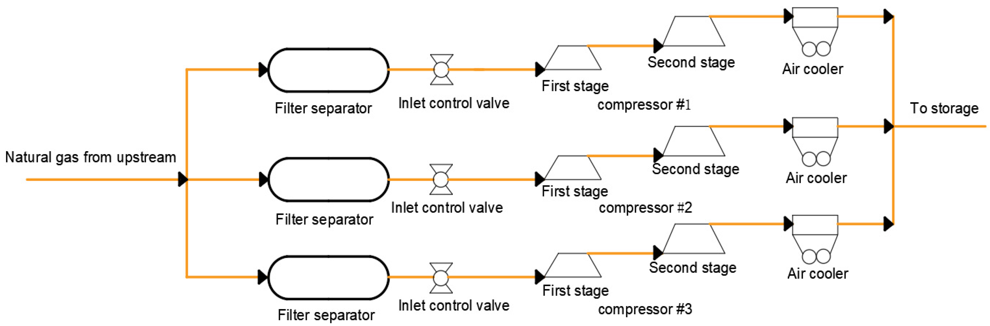
2. Basic Information of Gas Storage Facility

Taking the gas injection station of a certain gas storage facility as an example to study the energy-saving potential of the gas injection process, Figure 1 shows a schematic diagram of the injection process. The energy consumption of the three compressors and three air coolers in the injection station generally accounts for more than 96% of the total process energy consumption. By establishing a mathematical model for the parallel operation of multiple compressors and air coolers, a multi-objective optimization algorithm is used to calculate and solve the combinations of three compressors and air coolers with different performance, in order to determine the optimal operating method between the compressors and air coolers.

2.1. Basic Parameters of Compressors

The gas injection station of the gas storage facility is equipped with three double-acting reciprocating natural gas compressors, which operate in parallel to increase the injection capacity.

Table 1. Basic situation of a compressor at an injection station in a gas storage reservoir.

No.	#1	#2	#3
Rated Flow (×104 m3/d)	80	180	180
Suction Pressure (MPa)	4.5~7.5	4.5~7.5	4.5~7.5
Rated Discharge Pressure (MPa)	6.9~17	6.9~17	6.9~17
Actual Speed (r/min)	750~1000	750~1000	750~1000
Stages	2	2	2
Number of Cylinders	3	6	6
Rated Power (kW)	1324	3531	3532

presents the detailed basic parameters of the compressors. According to the field data, the actual intake pressure of the compressors fluctuates between 4.5 MPa and 6.5 MPa, with an average value of 5.41 MPa. The intake temperature varies between 10 °C and 25 °C, while the discharge pressure ranges from 10 MPa to 16.5 MPa, with an average discharge pressure of 11.50 MPa. These three compressors are each equipped with 15 kW, 55 kW, and 45 kW air coolers.

2.2. Basic Parameters of Air Coolers

The air coolers for the compressors in the gas storage facility studied in this paper are vertical blowers, arranged in parallel in three units. The air coolers mainly consist of core components (tube bundles, fans, and frames) and auxiliary components (louvers, ladder platforms, etc.). The core components cool the system by allowing air to flow transversely across the outside of the tube bundles to carry away heat. The fans enhance the airflow to improve heat exchange efficiency, while the louvers regulate the air direction and protect the finned tubes. The detailed structural parameters of the air coolers are shown in

Table 2. Basic structural parameters of the air cooler.

No.	#1	#2	#3
Fan Diameter (inches)	120	180	180
Number of Blades (pieces)	6	8	8
Number of Fans (pieces)	2	2	2
Blade Angle (°)	12	12	12
Piping Layout Method	Crossflow	Crossflow	Crossflow
Pipe Diameter (mm)	15.9	15.9	15.9
Pipe Length (m)	9.1	17.7	17.7
Finned Surface Area Ratio	15.9	15.9	15.9
Number of Tube Rows	3	3	3
Motor Rated Speed (r/min)	1450	1450	1500
Motor Rated Power (kW)	15	55	45

.

2.3. Natural Gas Composition

The natural gas composition at the compressor inlet is shown in

Table 3. Natural gas component.

Composition	Mole Fraction (%)
Methane	96.1
Ethane	1.74
Propane	0.58
Isobutane	0.28
Isopentane	0.03
N-hexane	0.09
Nitrogen	0.56
Carbon dioxide	0.62

. Considering the impact of the thermophysical properties of natural gas on the thermodynamic calculations of the compressor, this paper uses the REFPROP V10.0 database to obtain the thermophysical properties of natural gas to support subsequent model calculations [15].

3. System Optimization Models

All thermodynamic calculations and optimization processes in this study were implemented using Python 3.9. The thermophysical properties of natural gas were calculated using the NIST REFPROP 10.0 database, which was integrated into the Python environment via the ctREFPROP interface.

3.1. Compressor Mechanism Model

After years of operation, the performance of the compressors at the gas injection station of the gas storage facility significantly changes compared to their original factory specifications. As reciprocating compressors are core equipment in optimizing the gas injection process, it is essential to comprehensively understand the actual performance of the compressors under various conditions. To accurately obtain the actual performance of a single compressor under different operating conditions (such as discharge volume, first-stage discharge pressure, first-stage discharge temperature, and indicated power at each stage), this paper establishes a thermodynamic model for reciprocating compressors [16].

Table 4. Compressor model parameters.

Input Parameters	Structural Parameters	Output Parameters
First-Stage Suction Pressure First-Stage Suction Temperature Second-Stage Discharge Pressure Second-Stage Discharge Temperature	First-Stage Piston Stroke First-Stage Cylinder Diameter Second-Stage Piston Stroke Second-Stage Cylinder Diameter Piston Rod Diameter	Discharge Volume First-Stage Discharge Pressure First-Stage Discharge Temperature First-Stage Indicated Power Second-Stage Indicated Power

lists the specific input process parameters, structural parameters, and output process parameters for the model. The first-stage suction pressure is denoted as p_1s; suction temperature as T₁s; and second-stage discharge pressure and temperature as p_2d and T_2d, respectively. Structural parameters such as piston stroke and cylinder diameter are represented as S, D, and d with appropriate subscripts to indicate stage. Output parameters such as volumetric flow rate (q_v), discharge pressure (p_1d and p_2d), temperature (T_1d and T_2d), and indicated power (P₁ and P₂) are also consistently labeled.

3.1.1. Thermodynamic Model

The thermodynamic process of the compressor involves heat transfer and resistance issues when the compressed gas passes through the discharge valve. Therefore, in the thermodynamic calculations, the multi-stage compressor model is assumed to be a two-stage cylinder system in series, with the following necessary assumptions:

• Within the study period, the system operates under steady-flow conditions, and there are no performance differences among cylinders of the same stage.
• The natural gas undergoes an isenthalpic process when passing through various throttling valves, with no performance losses.
• Since the reciprocating compressor is not equipped with an intercooler, the discharge pressure and temperature of the first-stage compressor are considered as the intake pressure and temperature of the second-stage compressor, while inter-stage pressure losses are ignored.

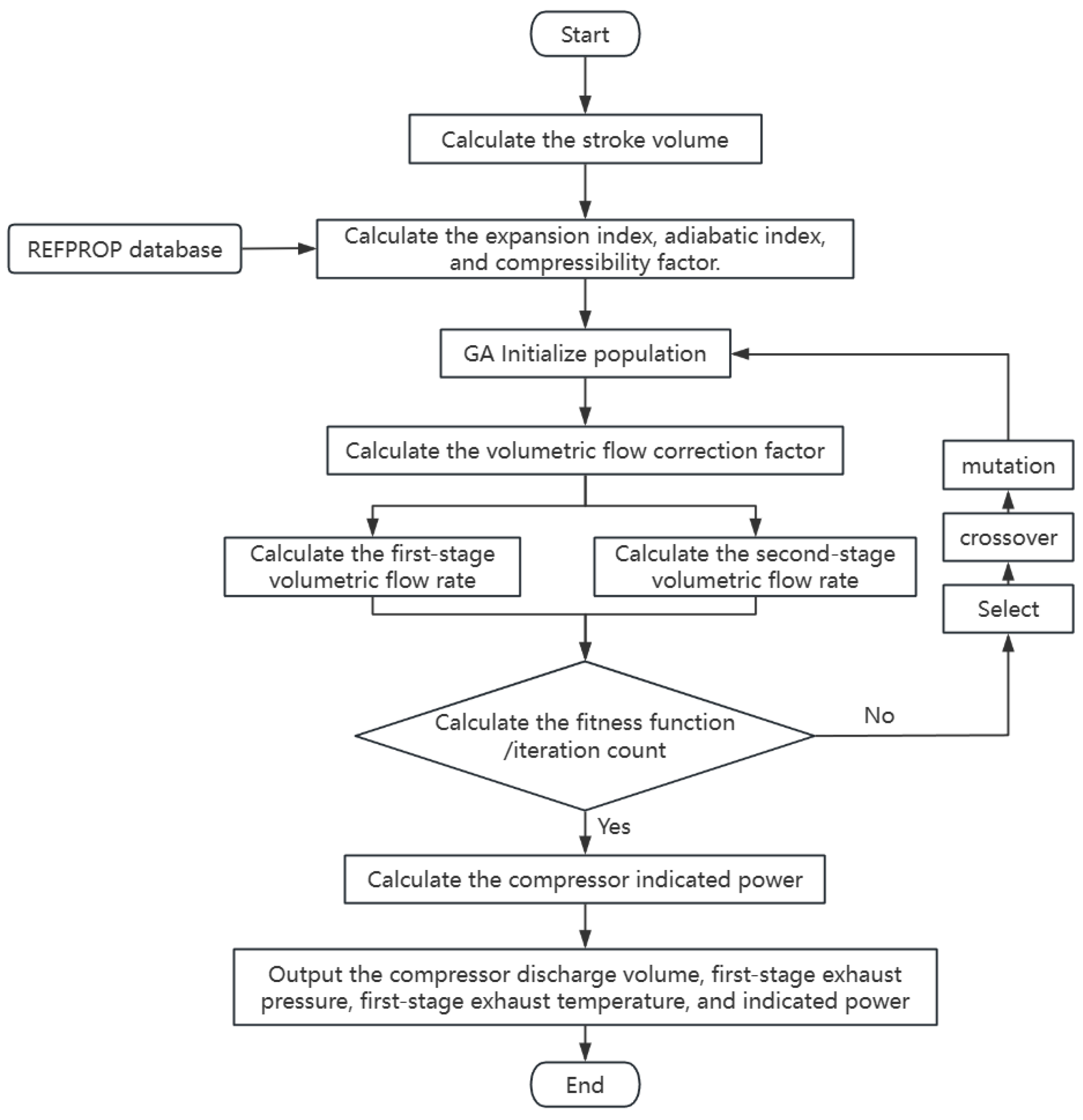
The nominal compression ratio is defined as follows:

$$\epsilon ={\displaystyle \frac{p_{\mathrm{out}}}{p_{\mathrm{in}}}}$$

(1)

In this equation, ε represents the nominal compression ratio of the compressor, and p_out and p_in are the absolute intake and discharge pressures, respectively, in MPa.

A double-acting reciprocating compressor is a type of compressor that operates with independent intake and discharge valves on both sides of the cylinder. As the piston moves to one side, it compresses the gas on that side while simultaneously increasing the volume; opposingly, the working volume of a double-acting cylinder is expressed as follows:

$$V_{\mathrm{s}}={\displaystyle \frac{1}{4}}\pi (2D^2-d^2)S$$

(2)

where V_s represents the working volume of the double-acting cylinder, in mm³; D is the cylinder diameter, in mm; d is the cylinder diameter, in mm; and S is the piston stroke, in mm.

During the actual operation of the compressor, not all of the compressed gas is completely discharged into the next stage. The volumetric efficiency is a physical quantity used to describe the difference between the actual intake volume of the compressor and the ideal intake volume in the compression cycle. Volumetric efficiency is expressed as follows:

$${\eta }_{\mathrm{v}}={\displaystyle \frac{V_{\mathrm{ds}}}{V_{\mathrm{s}}}}={\lambda }_{\mathrm{v}}{\lambda }_{\mathrm{p}}{\lambda }_{\mathrm{t}}{\lambda }_{\mathrm{L}}{\lambda }_{\phi }$$

(3)

where V_ds and V_s represent the actual intake volume and the ideal intake volume of the compressor, respectively. λ_V, λ_p, λ_T, λ_L, and λ_φ are the volumetric coefficient, pressure coefficient, temperature coefficient, leakage coefficient, and condensation coefficient, respectively. The detailed calculation method is listed in Appendix A.1.

For subsequent thermodynamic calculations, λ_V, λ_P, and λ_T are collectively referred to as the intake coefficient, which has the greatest impact on the volumetric efficiency of the compressor. The volumetric flow calculation method is as follows:

$$q_{\mathrm{v}}=V_{\mathrm{s}j}{\displaystyle \frac{{\lambda }_{\mathrm{v}j}{\lambda }_{\mathrm{p}j}{\lambda }_{\mathrm{t}j}{\lambda }_{\mathrm{L}j}}{{\lambda }_{\varphi j}{\lambda }_{\mathrm{c}j}}}{\displaystyle \frac{p_{\mathrm{s}j}}{p_{\mathrm{s}1}}}{\displaystyle \frac{T_{\mathrm{s}1}}{T_{\mathrm{s}j}}}{\displaystyle \frac{Z_{\mathrm{s}1}}{Z_{\mathrm{s}j}}}n$$

(4)

where n is the rotational speed of the compressor, and T_s1 and T_sj are the intake and discharge temperatures of the compressor cylinder, respectively.

The indicated power is expressed as follows:

$$P_i={\displaystyle \sum \frac{\mathrm{n}}{60}}\left(1-{\delta }_{\mathrm{s}}\right)p_1{\lambda }_{\mathrm{v}}{V}_{\mathrm{s}}{\displaystyle \frac{m}{m-1}}\left\{{\left[\epsilon \left(1+{\delta }_0\right)\right]}^{{\displaystyle \frac{m-1}{m}}}-1\right\}{\displaystyle \frac{Z_1+Z_2}{2Z_1}}$$

(5)

where P₁ represents the actual suction pressure, δs is the suction pressure loss, δ₀ is the total relative pressure loss, Z₁ is the compressibility factor at suction, Z₂ is the compressibility factor at discharge, and n is the polytropic index.

The actual indicated power of the compressor represents the energy consumption in kW required to process a unit volume of gas at a given intake pressure and temperature.

Mechanical efficiency is calculated as follows:

$$\begin{array}{l}{P}_{\mathrm{sh}}=P_{\mathrm{i}}+P_{\mathrm{f}}+P_{\mathrm{a}}\\ {\eta }_{\mathrm{m}}={\displaystyle \frac{P_{\mathrm{i}}}{P_{\mathrm{sh}}}}\end{array}$$

(6)

where P_sh is the power supplied to the compressor’s shaft by the drive motor, in kW. It mainly consists of three parts: the indicated power P_i of the compressor, the friction power P_f consumed by moving parts, and the power P_a required by the drive accessories. The mechanical efficiency of the compressor reflects the internal energy conversion efficiency and the level of perfection and is an important indicator for evaluating the design quality of the compressor.

For reciprocating compressors that are already in operation, the stroke volume of each cylinder can be calculated. Therefore, the relationship between the stroke volumes of adjacent cylinders (Equation (7)) can be used to derive the relationship between the suction pressure of any stage and the suction pressure of the first stage, and the inter-stage pressure can be corrected using Equation (8).

Inter-stage pressure correction is represented as follows:

$$V_{\mathrm{h}j}{\displaystyle \frac{{\lambda }_{\mathrm{v}j}{\lambda }_{\mathrm{p}j}{\lambda }_{\mathrm{t}j}{\lambda }_{\mathrm{L}j}}{{\lambda }_{\varphi j}{\lambda }_{\mathrm{c}j}}}{\displaystyle \frac{p_{\mathrm{s}j}}{p_{\mathrm{s}1}}}{\displaystyle \frac{T_{\mathrm{s}1}}{T_{\mathrm{s}j}}}{\displaystyle \frac{Z_{\mathrm{s}1}}{Z_{\mathrm{s}j}}}=V_{\mathrm{h}j+1}\cdot {\displaystyle \frac{{\lambda }_{\mathrm{v}j+1}{\lambda }_{\mathrm{p}j+1}{\lambda }_{\mathrm{t}j+1}{\lambda }_{\mathrm{L}j+1}}{{\lambda }_{\varphi j+1}{\lambda }_{\mathrm{c}j+1}}}{\displaystyle \frac{p_{\mathrm{s}j+1}}{p_{\mathrm{s}1}}}{\displaystyle \frac{T_{\mathrm{s}1}}{T_{\mathrm{s}j+1}}}{\displaystyle \frac{Z_{\mathrm{s}1}}{Z_{\mathrm{s}j+1}}}$$

(7)

$$p_{\mathrm{s}j}={\displaystyle \frac{V_{\mathrm{s}1}}{V_{\mathrm{s}j}}}{\displaystyle \frac{{\lambda }_{\mathrm{v}1}{\lambda }_{\mathrm{p}1}{\lambda }_{\mathrm{t}1}{\lambda }_{\mathrm{L}1}}{{\lambda }_{\mathrm{v}j}{\lambda }_{\mathrm{p}j}{\lambda }_{\mathrm{t}j}{\lambda }_{\mathrm{L}j}}}{\displaystyle \frac{{\lambda }_{\varphi j}{\lambda }_{\mathrm{c}j}}{{\lambda }_{\varphi 1}{\lambda }_{\mathrm{c}1}}}{\displaystyle \frac{T_{\mathrm{s}j}}{T_{\mathrm{s}1}}}{\displaystyle \frac{Z_{\mathrm{s}j}}{Z_{\mathrm{s}1}}}{p}_{\mathrm{s}1}$$

(8)

The calculation formula for the pressure ratio of each stage is as follows:

$$\left\{\begin{array}{l}{p}_{\mathrm{d}j}=p_{\mathrm{s}(j+1)}\hfill \\ {\epsilon }_j={\displaystyle \frac{p_{\mathrm{d}j}}{p_{\mathrm{s}j}}}\hfill \end{array}\right.$$

(9)

3.1.2. GA-BP Model

During the actual operation of the compressor, due to the temperature differences and varying geometric sizes of the two-stage cylinders, the inter-stage pressure of the real compressor is not evenly distributed according to the equal pressure ratio. Instead, it changes with the geometry of the cylinders, temperature, and the intake and discharge conditions. This paper applies a genetic algorithm to solve the nonlinear problem in the inter-stage pressure correction, transforming it into an optimization problem. This approach avoids local optimal solutions caused by improper initial value settings, thereby improving the accuracy of the thermodynamic model.

The genetic algorithm is used to optimize five key parameters in the compressor thermodynamic model, including inter-stage pressure, intake coefficients for each stage, and the polytropic index. The optimization of these parameters makes the model closer to the actual operating conditions, improving its adaptability under various conditions. This study found that when the population size is set to 15, the iteration limit is 400, the crossover probability is 0.7, the mutation probability is 0.1, and the predefined fitness termination threshold is 0.001, it balances computational speed and accuracy.

As shown in the Figure 2, the specific steps for calculating the compressor thermodynamic model using the genetic algorithm are as follows:

• Initialize the population

Genetic algorithms first need to initialize the population, where each individual in the population represents a solution to the equation. The traditional method for initializing the population is to use binary encoding for individuals, but this method is lengthy and cumbersome for defining the domain. To make the encoding physically meaningful, real-valued encoding is used. The individual’s gene sequence in the population is represented as follows:

$$g=(p_{\mathrm{d}1},c_1,c_2,n_1,n_2)$$

(10)

In this equation, p_d1 is the interstage pressure of the compressor, taken in the range of 6 to 11 MPag; c₁ is the first-stage intake coefficient, with a range of 0.91 to 0.96; c₂ is the second-stage intake coefficient, constrained to a range of 0.93 to 0.98; and n₁ and n₂ are the multi-variable indices for the first and second stages, constrained to the range of 1.32 to 1.41.

2.

Fitness function

The fitness function is defined as the sum of the squared differences in two-stage flow, with the goal of minimizing the function value to achieve optimal flow consistency. The calculation process of the fitness function involves evaluating each individual in the population, which represents a specific inter-stage pressure scheme. By comparing the fitness of each scheme, the pressure setting closest to the ideal flow consistency is identified.

$${(V_{\mathrm{h}j}{\displaystyle \frac{{\lambda }_{\mathrm{v}j}{\lambda }_{\mathrm{p}j}{\lambda }_{\mathrm{t}j}{\lambda }_{\mathrm{L}j}}{{\lambda }_{\varphi j}{\lambda }_{\mathrm{c}j}}}{\displaystyle \frac{p_{\mathrm{s}j}}{p_{\mathrm{s}1}}}{\displaystyle \frac{T_{\mathrm{s}1}}{T_{\mathrm{s}j}}}{\displaystyle \frac{Z_{\mathrm{s}1}}{Z_{\mathrm{s}j}}}-V_{\mathrm{h}j+1}{\displaystyle \frac{{\lambda }_{\mathrm{v}j+1}{\lambda }_{\mathrm{p}j+1}{\lambda }_{\mathrm{t}j+1}{\lambda }_{\mathrm{L}j+1}}{{\lambda }_{\varphi j+1}{\lambda }_{\mathrm{c}j+1}}}{\displaystyle \frac{p_{\mathrm{s}j+1}}{p_{\mathrm{s}1}}}{\displaystyle \frac{T_{\mathrm{s}1}}{T_{\mathrm{s}j+1}}}{\displaystyle \frac{Z_{\mathrm{s}1}}{Z_{\mathrm{s}j+1}}})}^2<0.001$$

(11)

3.

Genetic operations

Selection, crossover, and mutation operations together form the core of the genetic algorithm and are key to its effectiveness compared to other algorithms. The selection operation chooses the best individuals based on their fitness values to move on to the next generation. The crossover operation involves performing crossover on selected individuals to generate new ones. The mutation operation introduces small random changes to some individuals with a low probability, increasing the diversity of the population and preventing the algorithm from getting stuck in local optima.

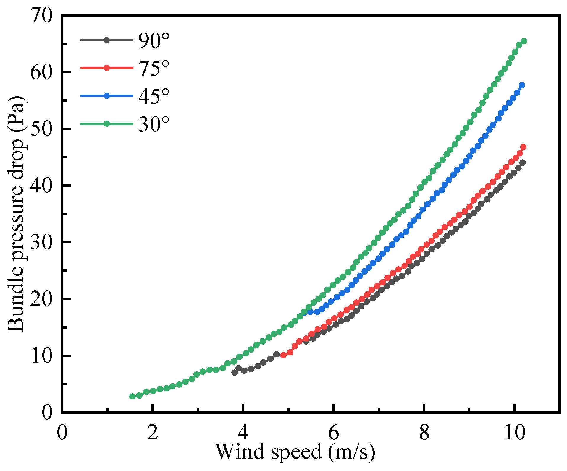
3.2. Air Cooler Flow and Heat Transfer Model

3.2.1. Flow Model

When the motor drives the fan blades to rotate, the blades push the surrounding air to flow. Similarly, the rotation of the blades is resisted by air drag, which increases the motor load and power consumption. The air cooler adjusts the airflow through the cooler by changing the louvers’ opening, thereby affecting the torque and power required by the motor. The flow model of the air cooler mainly involves calculating the airflow and the pressure drop when air flows through the fins [17]. To simplify the mathematical model, the following assumptions are made:

• Since the fan speed is relatively low, the variation in air density is negligible, and it can be treated as an incompressible fluid [18].
• The airflow over the air cooler is steady. In forced ventilation, the airflow generated by the fan passes entirely through the fins.
• The airflow generated by the fan is uniform, and the effects of the environment and structure on the fan airflow are neglected.

Thus, the blade tip speed can be expressed as follows:

$$V_{tip}={\displaystyle \frac{\pi Dn}{60}}$$

(12)

In this formula, D is the blade diameter in m and n is the fan rotational speed (r/min). Given that the blade angle θ is 12°, the axial velocity along the blade V_Z can be expressed as follows:

$$V_Z=V_{tip}\times tan{12}^{°}$$

(13)

The axial wind speed multiplied by the swept area of the blade gives the blade air volume:

$$Q_{\mathrm{air}}=A_{\mathrm{fans}}\times V_{\mathrm{Z}}\times \beta$$

(14)

where β is the blade correction factor, which is related to the structure of the blade. The power of the motor equipped with the fan in forced ventilation is as follows:

$$N={\displaystyle \frac{2.778\times {10}^{-7}HV{F}_{\mathrm{L}}}{{\eta }_1\cdot {\eta }_2\cdot {\eta }_3}}$$

(15)

In this formula, N is the motor power required by the fan, in kW; H is the total air pressure, in Pa; V is the actual air volume at the fan inlet, in m³·h; η₁ is the fan efficiency; η₂ is the belt transmission efficiency, taken as 0.95; η₃ is the motor efficiency; and F_L is the altitude correction factor, taken as 1.

As shown in

Table A2. Performance of fans and drive motors under different loads.

Equipment Load (%)	Fan Efficiency (%)	Motor Power Factor (%)
50	94.8	76.8
75	94.9	83.4
100	94.5	85.2

(in Appendix A.2), the fan efficiency remains nearly constant at different loads, while the motor power factor increases as the load increases. Therefore, maximizing the fan load can improve the motor’s energy conversion efficiency.

The fan pressure drop calculation ensures that air can pass through the fins at an appropriate speed during normal operation to guarantee heat exchange effectiveness. The fan pressure drop calculation mainly includes dynamic pressure calculation and static pressure calculation. The static pressure calculation includes air inlet resistance, fan protective net resistance, bundle inlet resistance, bundle outlet resistance, and bundle resistance. When the structure of the air cooler is determined, the bundle resistance accounts for the largest proportion [19,20,21]. Figure 3 shows the relationship between wind speed and static pressure of the air cooler at different louver openings, measured in the field. As shown in the figure, the higher the wind speed, the higher the static pressure of the air cooler. The larger the louver opening, the smaller the pressure drop. Taking air cooler #1 as an example, when the fan operates at full speed, the tip speed can reach 61 m/s, and the static pressure of the air cooler is approximately 70 Pa.

By solving Equations (18)–(22) simultaneously, the relationship between the power of the air cooler and the air volume can be derived as follows:

$$N={\displaystyle \frac{2.778\times {10}^{-7}{F}_{\mathrm{L}}}{{\eta }_1\cdot {\eta }_2\cdot {\eta }_3}}(\Delta p+{\displaystyle \frac{1}{2}}\rho {V_{\mathrm{z}}}^2)\times \pi \times ({\displaystyle \frac{D}{2}}{)}^2\times tan\theta \times {\displaystyle \frac{n\pi D}{60}}$$

(16)

In order to perform data modeling, the relationship between the wind speed of the compressor and the pressure drop of the heat exchanger in Figure 3 is fitted. The curve in the figure shows a gentle variation, and a cubic polynomial fit is applied. The evaluation criteria for the fit, including the sum of squared residuals and the square of the correlation coefficient, yield very good results, with the square of the correlation coefficient reaching 0.99, meeting the fitting requirements.

When the louver angle is 30°:

$$\Delta p=3.32-1.394V_Z+0.8{V_Z}^2-0.006{V_Z}^3$$

(17)

The fitting results are as follows: the sum of squared errors (SSE) is 3.93; the coefficient of determination (R²) is 0.996.

When the louver angle is 45°:

$$\Delta p=0.165+1.097V_Z+0.281{V_Z}^2+0.0168{V_Z}^3$$

(18)

The fitting results are as follows: the sum of squared errors (SSE) is 11.2; the coefficient of determination (R²) is 0.992.

When the louver angle is 75°:

$$\Delta p=-15.353+5.654V_Z-0.207{V_Z}^2+0.024{V_Z}^3$$

(19)

The fitting results are as follows: The sum of squared errors (SSE) is 1.46; the coefficient of determination (R²) is 0.995.

When the louver angle is 90°:

$$\Delta p=9.482-4.078V_Z+{V_Z}^2-0.0264{V_Z}^3$$

(20)

The fitting results are as follows: the sum of squared errors (SSE) is 2.97; the coefficient of determination (R²) is 0.994.

3.2.2. Heat Transfer Model

The heat exchange process of the compressor aftercooler can be divided into three parts. First, convective heat transfer occurs between the natural gas inside the tube and the tube wall. Second, heat conduction takes place from the tube wall to its outer surface and fins. Finally, external cold air removes heat from the fins and outer surface through forced convection [22]. Figure 4 specifically describes the heat exchange process between the outer tube bundle of the air cooler and the air. Figure 4a shows the structural schematic, while Figure 4b presents the temperature profiles of the hot and cold fluids, indicating the variation in temperature difference between natural gas inside the tubes and the air outside. The inlet and outlet temperatures of high-temperature natural gas are denoted by T₁ and T₂, while the inlet and outlet temperatures of air are represented by t₁ and t₂. Considering that the heat transfer mechanism of finned surfaces in the air cooler is relatively complex and that this study aims to explore the relationship between heat exchange efficiency and energy consumption, the heat transfer model is simplified as follows to eliminate unnecessary computational complexity:

• The entire heat transfer process is in a steady state.
• The contact thermal resistance between the fins and the tubes is neglected [23].
• The effect of thermal radiation from the environment is ignored, and the thermal conductivity of the fins is considered constant.
• The natural gas inside the heat exchanger is assumed to flow uniformly through all tube bundles.
• The airflow provided by the fan is uniform, and the position of the tube bundles has no significant impact on the heat exchange performance.
• The air velocity is constant, meaning that variations in forced convection heat transfer outside the tubes are minimal. This allows for reasonable simplifications of the heat exchange process to facilitate data fitting and calculations.

The fundamental heat transfer equation for the thermal performance of the tube bundle in the air cooler is as follows:

$$Q=KA\Delta T_{\mathrm{m}}$$

(21)

where Q is the heat load of the tube bundle, in kJ; K is the overall heat transfer coefficient of the tube bundle, in kJ/(m²·K); A is the total heat transfer area of the tube bundle, in m²; and ΔT_m is the logarithmic mean temperature difference, in °C.

The logarithmic mean temperature difference for crossflow heat exchange in the air cooler can be expressed as follows:

$$\Delta T_{\mathrm{m}}=\psi \cdot \Delta T_{\mathrm{lm}}$$

(22)

$$\Delta T_{\mathrm{lm}}={\displaystyle \frac{(T_1-t_2)-(t_1-T_2)}{\ln \frac{(T_1-t_2)}{(t_1-T_2)}}}$$

(23)

where $\psi$ is the temperature correction factor, which is taken as 0.92 in this study.

The external heat transfer area of the tube bundle can be simply divided into two parts: one is the surface area of the bare tube, and the other is the finned surface area. The bare tube surface area is calculated as the product of the tube bundle’s outer perimeter and its length. Multiplying this value by the finning ratio gives the total heat transfer area of the heat exchanger.

According to heat transfer theory [22], when there is no phase change in the fluids on both sides of the air cooler, the heat balance equation for the heat exchange process between the hot and cold fluids can be expressed as follows:

On the air side outside the tubes:

$$Q_{\mathrm{air}}=q_{\mathrm{mair}}\cdot C{p}_{\mathrm{air}}\cdot (t_2-t_1)$$

(24)

On the natural gas side inside the tubes:

$$Q_{\mathrm{gas}}=q_{\mathrm{mgas}}\cdot \mathrm{C}{p}_{\mathrm{gas}}\cdot (T_1-T_2)$$

(25)

In this equations, q_mgas is the mass flow rate, in kg/m³, and Cp is the specific heat capacity of the gas at constant pressure, in kJ/(kg·K). Under steady-state operation, the heat exchanged between the hot and cold fluids is equal, meaning that Equations (21), (24) and (25) are equal.

Based on the historical data from the gas storage facility, the flow rate of natural gas and its inlet and outlet temperatures can be obtained. Therefore, the total heat transfer coefficient of the heat exchanger can be expressed as follows:

$$K={\displaystyle \frac{Q}{A\frac{(T_1-t_2)-(t_1-T_2)}{\ln \frac{(T_1-t_2)}{(t_1-T_2)}}}}$$

(26)

Using the traditional empirical experimental correlation method to calculate the total heat transfer coefficient, the entire heat transfer coefficient can be divided into five parts. The total heat transfer coefficient can be expressed as follows [22]:

$$K={\displaystyle \frac{1}{\frac{1}{h_{\mathrm{in}}}\frac{d_{\mathrm{out}}}{d_{\mathrm{in}}}+\frac{d_{\mathrm{out}}}{2\lambda }\ln \frac{d_{\mathrm{out}}}{d_{\mathrm{in}}}+\frac{1}{h_{\mathrm{out}}}+R_{\mathrm{out}}+R_{\mathrm{in}}}}$$

(27)

In the above equation, h represents the convective heat transfer coefficient, in W/(m²·K); λ represents the thermal conductivity of the round tube, in W/(m·K); d represents the fouling thermal resistance, in (m²·K)/W; and the subscripts “out” and “in” refer to the outer and inner surfaces of the tube, respectively.

For the case of convective heat transfer on the outer surface of the tube, the traditional empirical formula method involves selecting an appropriate experimental correlation based on the Reynolds number. This is because the criteria numbers vary at different Reynolds numbers. Therefore, depending on the Reynolds number, the corresponding experimental correlation should be chosen for the calculation.

$$Re={\displaystyle \frac{ud}{\nu }}$$

(28)

In this formula, u represents the characteristic velocity, which is taken as the velocity of the air passing through the bent tube (m/s); d is the characteristic length, taken as the diameter of the bent tube (m); and ν is the kinematic viscosity of the fluid inside the finned tube (Pa·s).

The forced convection heat transfer coefficient under forced ventilation conditions for finned tubes, when the Reynolds number is in the range of 1~2 × 10⁶, is commonly calculated using the Briggs and Young formula:

$$Nu=0.134R{e}^{0.681}P{\mathrm{r}}^{1/3}(l/b{)}^{0.2}(l/\tau {)}^{0.1134}$$

(29)

where Nu is the Nusselt number for air flowing through the finned tube bundle, Pr is the Prandtl number, l is the fin spacing in m, b is the fin height in m, and τ is the fin thickness in m.

Prandtl number:

$$Pr={\displaystyle \frac{Cp\mu }{\lambda }}$$

(30)

where Cp is the specific heat capacity at constant pressure of the gas, in kJ/(kg·K); μ is the viscosity of air, in Pa·s; and λ is the heat transfer coefficient on the air side, in W/(m·K).

Nusselt number:

$$Nu={\displaystyle \frac{hl}{\lambda }}$$

(31)

where h is the convective heat transfer coefficient on the outer surface of the pipe, in W/(m·K), and l is the characteristic length, which in this case, is the outer diameter of the pipe, in m.

The convective heat transfer coefficient on the outer surface can thus be expressed as follows:

$$h_{\mathrm{out}}={\displaystyle \frac{0.134R{e}^{0.681}P{\mathrm{r}}^{1/3}{(l/b)}^{0.2}(l/\tau {)}^{0.1134}\lambda }{d}}$$

(32)

The fouling thermal resistance of the air cooler is taken as 3.52 × 10⁻⁴ m²·K/W based on the manufacturer’s guidance data for the air cooler, for all three air coolers.

3.3. NSGA-II Optimization Model

The load distribution optimization problem for three reciprocating compressors with different performances and three air coolers in the gas storage facility’s pressurization process is a typical multi-objective optimization problem (MOP). On one hand, it needs to meet the gas injection requirements while minimizing energy consumption and, at the same time, reduce the compressor’s outlet gas temperature to meet process requirements. The core of this problem is to achieve the best balance between maximum gas injection and minimum energy consumption while satisfying on-site process requirements. Since minimizing energy consumption and maximizing gas injection are conflicting objectives, this paper uses the “Pareto front” method to find solutions. The Pareto front consists of all potential optimal solutions, which require that all solutions first meet the constraints and then optimize the objective function values.

Based on evolutionary algorithms, strategies such as non-dominated sorting and crowding distance calculation are introduced to specifically solve multi-objective optimization problems. The NSGA-II is selected as the solution due to its efficient performance and ability to broadly cover the Pareto front. This optimizes the calculation accuracy and effectively balances the objectives of maximizing gas injection and minimizing energy consumption, providing a reliable optimization strategy for the compressor and air cooler load distribution in the gas storage facility’s pressurization process.

3.3.1. Objective Function

Under the condition of meeting on-site process requirements, it is necessary to establish a reasonable operating scheme that maximizes the gas injection volume while minimizing energy consumption. The method for establishing the compressor unit model has been described. Therefore, the objective function for optimization is the gas injection volume of the compressor unit and the energy consumption of the entire gas injection process [24].

• Gas injection volume of the compressor:

$$\max Q=a_1{Q}_1+a_2{Q}_2+a_3{Q}_3$$

(33)

2.

Total power of the gas injection process:

$$\min E=a_1{f}_1+a_2{f}_2+a_3{f}_3+a_1{k}_1+a_2{k}_2+a_3{k}_3+A$$

(34)

In this formula, a₁, a₂, and a₃ can only take values of 0 or 1, representing the operation (1) or shutdown (0) of equipment; f represents the energy consumption of the compressor, in kW; k represents the energy consumption of the air cooler, in kW; and A represents the energy consumption of other auxiliary equipment in the gas injection process, in kW, such as lubrication pumps, cooling water pumps, and compressor control systems (UCP). Once the compressor is running, these auxiliary devices must continue to operate to ensure normal functioning of the compressor.

Table A3. Energy consumption data for compressor ancillary equipment.

Energy Consumption Equipment	Parameters
Compressor oil injector pump motor	361 W/380 V/3 PH/50 Hz
Compressor pre-lubrication oil pump motor	3.75 KW/380 V/3 PH/50 Hz
Crankcase heater	2 × 2 KW/220 V/1 PH/50 Hz
Oil injector tank heater	3 × 150 W/220 V/1 PH/50 Hz
Compressor packing cooling water pump	0.75 KW/380 V/3 PH/50 Hz
Drive motor space heater	82 W/220 V/1 PH/50 Hz
UCP (UPS power supply)	1.87 KW/220 V/1 PH/50 Hz
Electric trace heating	8 W/220 V/50 Hz

in Appendix A.1 lists the energy consumption data for the main auxiliary equipment.

3.3.2. Constraints

The compressor’s power consumption and injection volume are both influenced by the inlet and outlet pressure and temperature. Meanwhile, to meet the outlet temperature requirement, the temperature of the air cooler should not exceed 55 °C. If the air cooler temperature exceeds 55 °C, the compressor speed needs to be adjusted to reduce the compressor injection volume and power consumption. Additionally, the operational conditions of the compressor must be met, making the overall constraint conditions quite complex. The constraint conditions are as follows:

• Compressor power consumption:

$$\begin{array}{l}0 \mathrm{kW}\le f_1\le 1324 \mathrm{kW}\\ 0 \mathrm{kW}\le f_2\le 3531 \mathrm{kW}\\ 0 \mathrm{kW}\le f_3\le 3532 \mathrm{kW}\end{array}$$

(35)

2.

Compressor speed:

$$\begin{array}{l}750 \mathrm{rpm}\le n_1\le 1000 \mathrm{rpm}\\ 750 \mathrm{rpm}\le n_2\le 1000 \mathrm{rpm}\\ 750 \mathrm{rpm}\le n_3\le 1000 \mathrm{rpm}\end{array}$$

(36)

3.

Fan cooler speed:

$$\begin{array}{l}0 \mathrm{rpm}\le F{n}_1\le 362 \mathrm{rpm}\\ 0 \mathrm{rpm}\le F{n}_2\le 255 \mathrm{rpm}\\ 0 \mathrm{rpm}\le F{n}_3\le 242 \mathrm{rpm}\end{array}$$

(37)

4.

Process parameter range:

$$\begin{array}{l}5 °\mathrm{C}\le T_0\le 25 °\mathrm{C}\\ 4.5 \mathrm{MPa}\le P_0\le 6.0 \mathrm{MPa}\\ 11 \mathrm{MPa}\le P_0\le 17 \mathrm{MPa}\end{array}$$

(38)

3.3.3. NSGA-II Model Parameters

Through continuous tuning of the initial parameters of the NSGA-II [25], the final settings were a population size of 50; a maximum iteration limit of 400; a heat exchanger calculation error of 5000 kJ/D; crossover probability and mutation probability of 0.9 and 0.2, respectively; a tolerance of 1 for decision variables; and a tolerance of 100 for constraint violations. This setup allows for a balance between calculation speed and accuracy.

Traditional genetic algorithms typically use a single fitness value to evaluate the quality of individuals. When there is a single objective function without other constraints, this method becomes efficient. However, when multiple objective functions and constraints exist, the solutions produced by genetic algorithms may end up being locally optimal, and they fail to cover the values across the Pareto front.

The calculation process of the NSGA-II algorithm [4] is shown in Figure 5. The NSGA-II has made the following improvements based on the genetic algorithm:

• Introduced non-dominated sorting and crowding distances to evaluate the quality of individuals, allowing the algorithm to better handle multi-objective optimization problems.
• Used a selection strategy based on the non-dominated sorting and crowding distances, enabling the algorithm to select better individuals.
• Maintained population diversity through the crowding distance, allowing the algorithm to find a broader range of solutions. An elitist strategy was used to ensure that excellent individuals from the previous generation are retained.

4. Results and Discussion

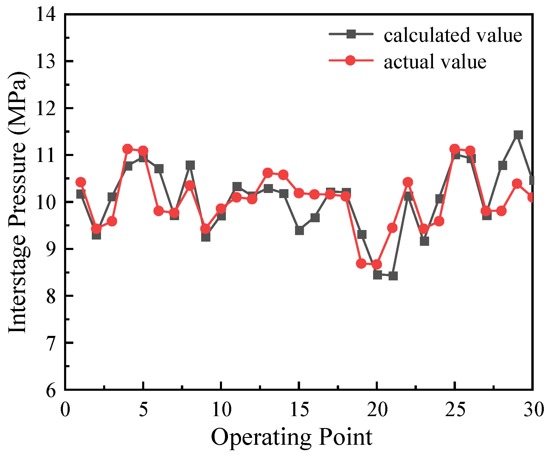
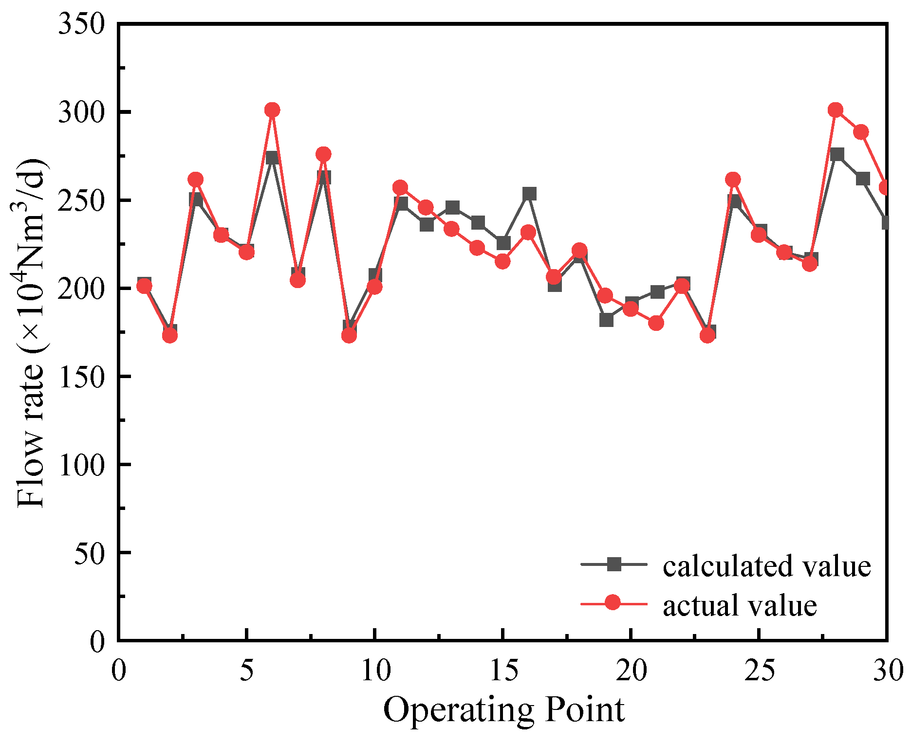
4.1. Validation of the Compressor Thermodynamic Model

Compressor #2 has been operating independently for a long period. Utilizing its standalone operation data can effectively eliminate data errors caused by interference from other units during parallel operation. To verify the accuracy of the proposed model, this study compares the results of the thermodynamic model optimized by the genetic algorithm with actual data under 30 different operating conditions based on the historical operating data of Compressor #2.

The comparison results of the interstage pressure and the processed gas volume calculated by the genetic algorithm with actual values are shown in Figure 6 and Figure 7. The results indicate that the maximum relative error between the calculated and actual interstage pressure does not exceed 5.5%, with an average relative error of 3.76%. Meanwhile, the maximum relative error between the calculated and actual processed gas volume does not exceed 8.9%, with an average relative error of 4.02%. The error in the calculated discharge volume is larger than that of the interstage pressure because the discharge volume is derived based on the interstage pressure, leading to a relatively higher error.

4.2. Thermodynamic Performance Analysis of the Compressor

This section provides a detailed analysis of the actual impact of key parameter variations on the performance of the reciprocating compressor. By using the controlled variable method, the inlet and outlet pressures, discharge temperature, and natural gas composition parameters are set to study the actual performance of the three compressors.

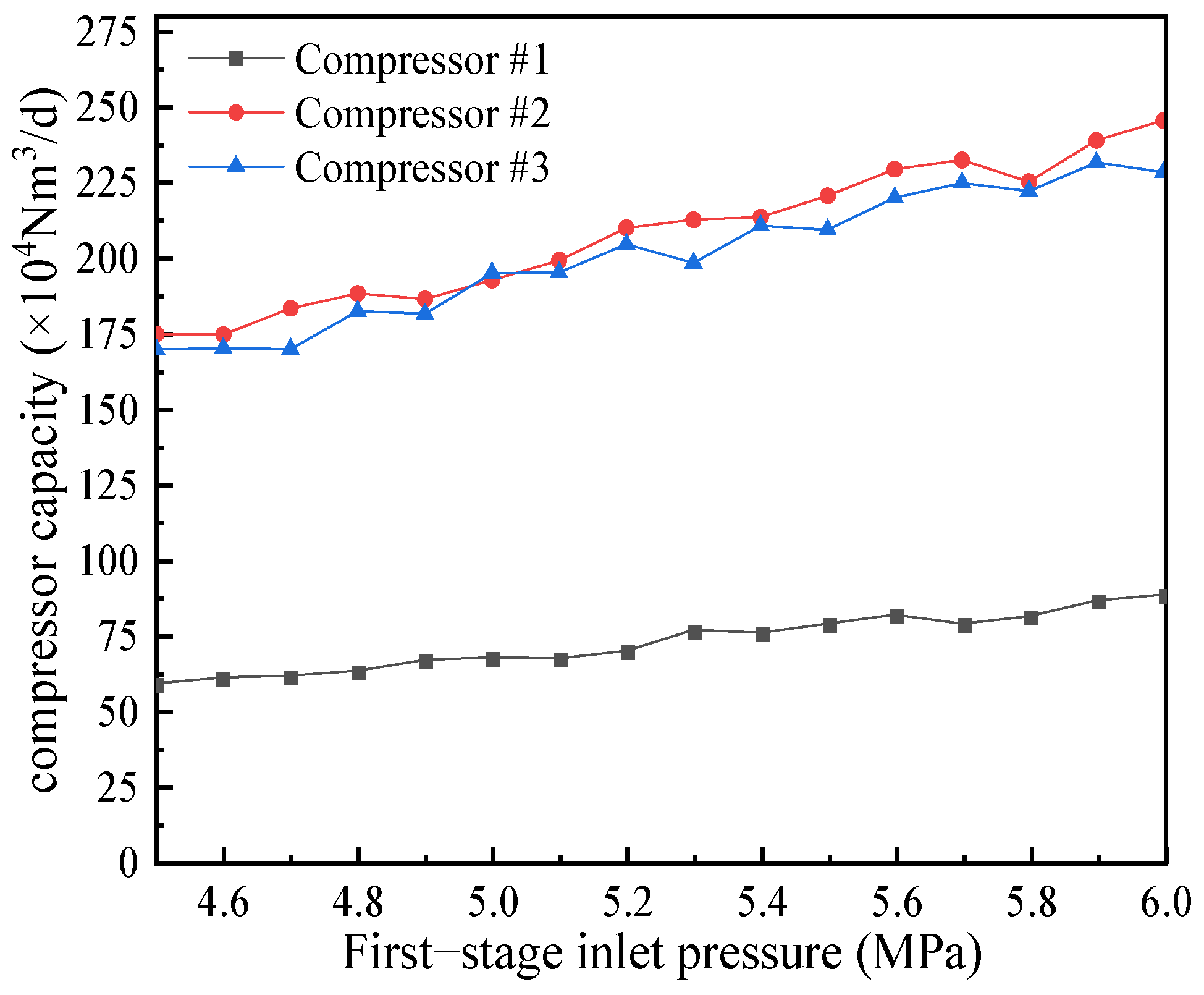
4.2.1. Effect of First-Stage Inlet Pressure

According to historical data, the compressor’s inlet pressure ranges from 4.5 to 6.0 MPa. Therefore, the inlet pressure gradient is set to 0.1 MPa, with an inlet temperature of 15 °C and a uniform discharge pressure of 14 MPa. The molar composition of natural gas at the compressor inlet is calculated according to Table 3, and the compressor speed is set to 1000 r/min. The processed gas volume and specific energy consumption of the three compressors under different inlet pressures are shown in Figure 8 and Figure 9.

Figure 8 illustrates the variation in compressor volumetric flow rate with changes in the first-stage inlet pressure. It can be observed that the inlet pressure has a significant impact on the compressor’s volumetric flow rate. Under the same discharge pressure, for every 0.1 MPa increase in the inlet pressure, the processed gas volume increases by approximately 2 × 10⁴ Nm³/D for Compressor #1 and by approximately 4.7 × 10⁴ Nm³/D for Compressor #2 and #3. This is because an increase in first-stage inlet pressure allows more natural gas to enter the first-stage cylinder of the compressor.

At the same time, Figure 9 shows that as the first-stage inlet pressure increases, the specific energy consumption of the compressor decreases significantly. The specific energy consumption of Compressor #1 is reduced by approximately 1.5 × 10⁻² kWh/Nm³, while for Compressor #2 and #3, it is reduced by approximately 1 × 10⁻² kWh/Nm³. The comparison in Figure 6 also indicates that Compressor #1 has the highest specific energy consumption under the same conditions, suggesting that it has the poorest economic performance. Compressor #2 and #3 exhibit similar performance; however, although they are of the same model and operating under identical conditions, Compressor #2 is more energy-efficient.

By analyzing the on-site operational data, it is found that the second-stage discharge temperature of Compressor #3 is higher than that of Compressor #2, indicating that more useful work is converted into heat in Compressor #3, leading to increased energy consumption.

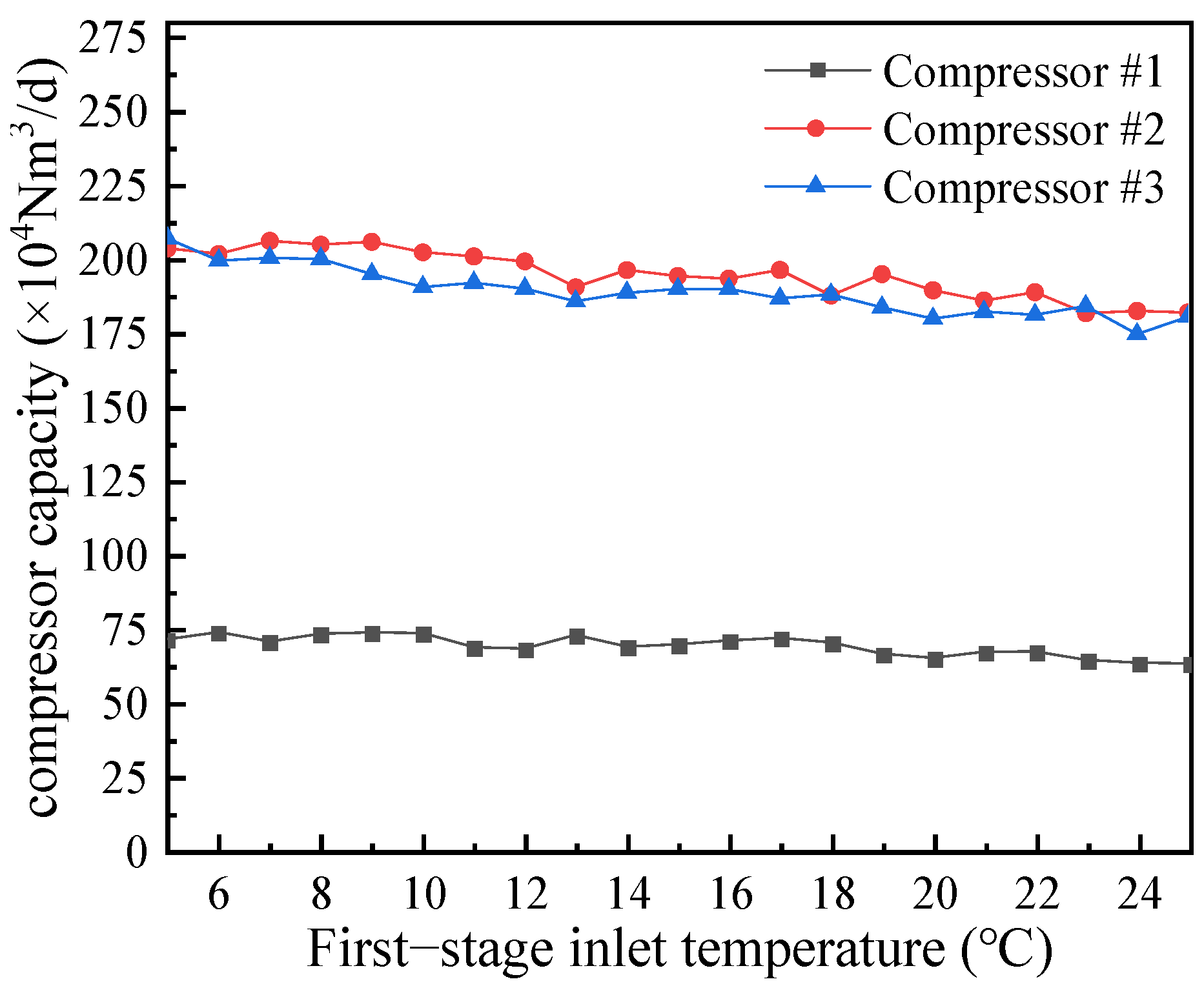
4.2.2. Effect of First-Stage Temperature

The compressor intake pressure is set to 5.0 MPa, the discharge pressure is 15 MPa, and the intake temperature ranges from 5 to 25 °C, with a temperature gradient set to 1 °C. The molar composition of natural gas at the compressor inlet is calculated according to Table 2, and the compressor speed is 1000 r/min. The calculated results for the gas handling capacity and specific energy consumption of the three compressors at different intake temperatures are shown in Figure 10 and Figure 11.

Compared to the impact of first-stage intake pressure on the compressor’s gas handling capacity, the effect of intake temperature on the compressor is relatively smaller. Within the intake temperature range of 5 to 25 °C, the gas handling capacity decreases as the temperature increases: the gas handling capacity of Compressor #1 drops from 71 × 10⁴ Nm³/D to 63 × 10⁴ Nm³/D, a reduction of 11%; meanwhile, Compressor #2 and #3 have their gas handling capacities reduced by approximately 22 × 10⁴ Nm³/D and 27 × 10⁴ Nm³/D. This result indicates that changes in intake temperature cannot be ignored when considering the compressor’s performance.

Based on the historical operation data, it can be observed that the discharge temperature of Compressor #3 is higher than that of Compressor #2, and the increase in temperature results in a lower gas density, which affects the compressor’s gas handling capacity. From Figure 10, it can be seen that Compressor #2 is more economical, and the unit energy consumption of the smaller Compressor #1 is much higher than that of Compressor #2 and #3. Reducing the intake temperature of the compressor is of significant importance for energy savings in reciprocating compressors.

4.2.3. Effect of Second-Stage Discharge Pressure

The secondary discharge pressure is set differently from the compressor’s primary suction pressure. Due to the process characteristics of the compressor, the suction pressure has a narrow range, while the discharge pressure, which is connected to the gas well of the storage reservoir, can vary more significantly. According to historical operation data, the backpressure of the compressor ranges from 11 to 17 MPa, with a pressure gradient set at 0.5. The suction pressure is set at 5 MPa, and the suction temperature is set at 15 °C. The impact of the compressor’s discharge pressure on its performance is then studied.

Figure 12 and Figure 13 show the impact of secondary discharge pressure on the compressor’s gas processing capacity and unit energy consumption. As the discharge pressure increases, the gas processing capacity gradually decreases, but the effect of discharge pressure on the gas processing capacity is quite limited: the gas processing capacity of Compressor 1 decreases by only 2 × 10⁴ Nm³/D, that of Compressor 2 decreases by only 22 × 10⁴ Nm³/D, and that of Compressor #3 decreases by only 19 × 10⁴ Nm³/D. This is because the thermodynamic model of the compressor is based on the assumption that the compressor’s gas valve seals are in good condition, with no backflow phenomenon, and the gas entering the first-stage cylinder is fully transferred to the second-stage cylinder. Therefore, the compressor’s gas processing capacity is mainly determined by the intake pressure rather than the discharge pressure.

As the discharge pressure increases, the overall unit energy consumption of the unit increases significantly. When the secondary discharge pressure is 11 MPa, the unit energy consumption of Compressor #1 is only 2.86 × 10⁻² kWh/Nm³. When the discharge pressure rises to 17 MPa, the unit energy consumption quickly increases to 4.33 × 10⁻² kWh/Nm³, an increase of approximately 1.5 times. Compressor #2 and #3 follow the same trend, with unit energy consumption increasing by 1.69 and 1.78 times. According to the compressor shaft power calculation formula, an increase in discharge pressure means the compressor needs to do more work, causing the power of the second-stage cylinder to rise rapidly, resulting in an increase in overall unit energy consumption.

4.3. NSGA-II Optimization Results

In order to align with actual field requirements, based on the typical pressure range in the on-site operation data, this study divides the operating states of the compressors into three different conditions: high pressure ratio, medium pressure ratio, and low pressure ratio. These three conditions are applied to the NSGA-II multi-objective optimization model, with the aim of exploring the compressor matching operation and multi-objective optimization operating strategy under various power demands. When using the NSGA-II algorithm for calculations, it is assumed that the compressor’s handling gas volume is adjusted by regulating the compressor’s speed.

4.3.1. High-Pressure-Ratio Operation

First, the operating conditions of the compressor under high-pressure-ratio conditions are analyzed. In this condition, the compressor’s inlet pressure is at its lowest and the discharge pressure is at its highest, resulting in maximum compressor load, while the air cooler is also operating at full capacity. The compressor inlet pressure is set to 4.5 MPa, discharge pressure is set to 17 MPa, and inlet temperature is set to 10 °C. The Pareto front graph of the startup and shutdown scheme for the three parallel compressors is obtained through calculations, as shown in Figure 14.

As the compressor speed increases, the air cooler speed increases synchronously. When the compressor speed reaches its maximum, the air cooler operates at full load. For every 250 r/min increase in compressor speed, the power of the #1 air cooler increases to 2.6 times its original value, mainly due to the increased wind resistance caused by the higher fan speed, leading to a significant rise in power consumption. At high speeds, the power consumption of the #1 air cooler accounts for 1.1% of the total gas injection process energy consumption, rising to 2.2%, while the #2 air cooler increases from 2.1% to 3.7%. This indicates that high-speed operations significantly increase the power consumption of the air cooler, which has a greater impact on overall energy consumption. Therefore, the operation strategy should be optimized to control energy consumption.

4.3.2. Medium-Pressure-Ratio Operation

The Pareto front of the start–stop scheme for the three parallel compressors is shown in Figure 15, calculated with the compressor inlet pressure set to 5 MPa, discharge pressure set to 14 MPa, and inlet temperature set to 10 °C.

Under the medium-pressure-ratio condition, the power consumption of the air cooler at the optimal speed is much lower compared to that under the high pressure ratio. The power consumption of the #1 air cooler as a proportion of the total energy consumption of the injection process increases from 0.3% to 0.56%, while the power consumption proportion of the #2 air cooler increases from 1.2% to 2.2%. Adjusting the speed of the #1 air cooler can achieve an energy consumption reduction of up to 3.2%. When adjusting the speed of the #2 air cooler, the energy-saving effect is even more significant, reaching up to 4.6%. Even when the compressor operates at 1000 r/min, adjusting the speed of the #2 air cooler can still achieve a 2.1% energy saving effect. This indicates that the energy-saving potential under the medium-pressure-ratio environment is greater than that under the high-pressure-ratio condition. The reason is that even under maximum load, the air cooler does not need to run at full speed to achieve the highest natural gas outlet temperature, providing greater energy-saving opportunities.

4.3.3. Low-Pressure-Ratio Operation

The Pareto front diagram of the start–stop scheme for the three parallel compressors is shown in Figure 16, calculated with the compressor inlet pressure set to 5.5 MPa, discharge pressure set to 11 MPa, and inlet temperature set to 10 °C.

Under low-pressure-ratio conditions, the compressor processes a large amount of gas with minimal power consumption, and the power consumption of the air cooler is very low. The speed of the #1 air cooler is only 20% of its full-speed operation, while the speed of the #3 air cooler is only 28% of its full-speed operation. Because the #1 and #3 air coolers are of different models, the #1 air cooler operates at a higher speed, resulting in a lower optimal air cooler speed under low-pressure conditions and better economic performance of the air cooler. The energy-saving effect brought by adjusting the air cooler speed is more significant. The theoretical calculations show that adjusting the speed of the #1 air cooler within the compressor operating range can save 1.6% to 4.3% of energy. Adjusting the speed of the #2 air cooler can save 5.89% to 7.9%. This is because under low-pressure-ratio conditions, the compressor’s outlet temperature is not high, and the air cooler can meet the requirement that the natural gas maximum discharge temperature does not exceed 55 °C with extremely low power consumption.

4.4. Compressor Unit Operation Plan

The NSGA-II algorithm was used to determine the startup and shutdown schemes for compressors under different operating conditions, as well as the matching of compressor and air cooler speeds. The conclusions indicate that selecting the appropriate combination of compressors or air coolers for different daily gas injection volumes can reduce the energy consumption of the injection process. The multi-unit operation scheme is shown in

Table 5. Operation plan for gas storage compressors.

Operating Condition	Daily Gas Injection Volume Range (×104 Nm3)	Compressor Start up Plan
High Pressure Ratio	<66	Compressor #1
	67~140	No optimal energy-saving plan; Compressor #3 can be started to shorten the operation time of Compressor #1
	145~194	Compressor #3
	195~261	Compressor #1 and #3
	291~388	Compressor #2 and #3
	>398	Compressor #1, #2, and #3
Medium Pressure Ratio	<74	Compressor #1
	74~168	No optimal energy-saving plan; Compressor #2 can be started to shorten the operation time of Compressor #1
	168~219	Compressor #3
	223~297	Compressor #1 and #3
	339~447	Compressor #2 and #3
	>456	Compressor #1, #2, and #3
Low Pressure Ratio	<85	Compressor #1
	85~190	No optimal energy-saving plan; Compressor #2 can be started to shorten the operation time of Compressor #1
	190~253	Compressor #3
	254~338	Compressor #1 and #3
	379~505	Compressor #2 and #3
	>516	Compressor #1, #2, and #3

. There are certain numerical gaps in the interval divisions, which are caused by the model or the compressor energy consumption optimization strategy. By comparing different compression ratios and gas injection demands, compressor scheduling can be further optimized to achieve energy-saving and consumption-reduction goals.

5. Conclusions

This study focuses on the parallel operation of multiple reciprocating compressors during the gas injection process in underground gas storage. A multi-objective optimization model was established, and the NSGA-II algorithm was employed to optimize the startup scheme of the compressors and the speed matching of the air coolers under different operating conditions. The main conclusions are as follows:

• A thermodynamic model for reciprocating compressors and a flow–heat transfer model for air coolers were developed, establishing a quantitative relationship between the air volume, power consumption, and fan speed of the air coolers. The energy consumption characteristics of air coolers were revealed, showing a significant nonlinear relationship between compressor power and speed. As the compressor speed approaches its maximum, the power consumption of the air coolers increases more rapidly.
• The effects of suction pressure, suction temperature, and discharge pressure on compressor performance were analyzed. The results indicate that increasing the suction pressure while reducing the suction temperature and discharge pressure can enhance the compressor’s gas handling capacity and reduce energy consumption.
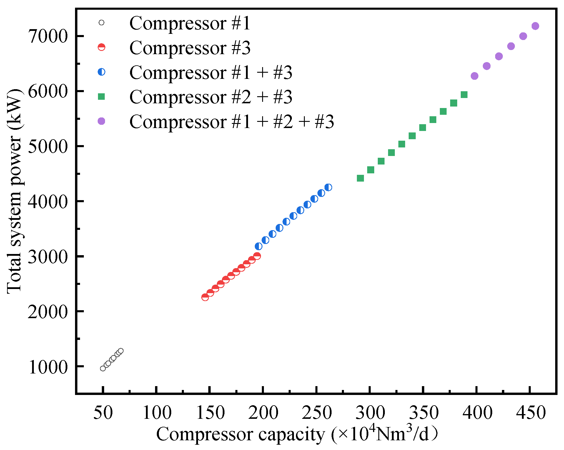
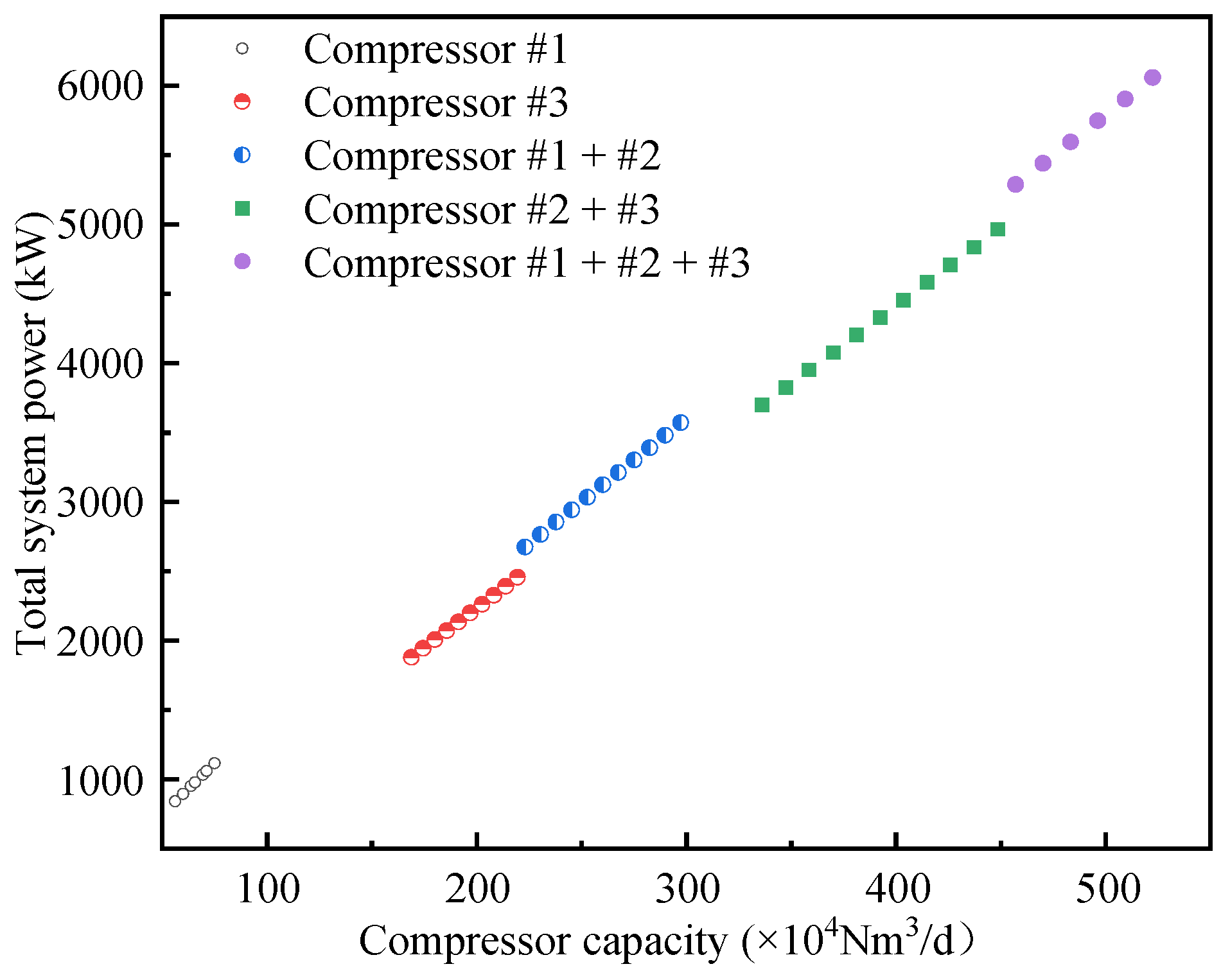
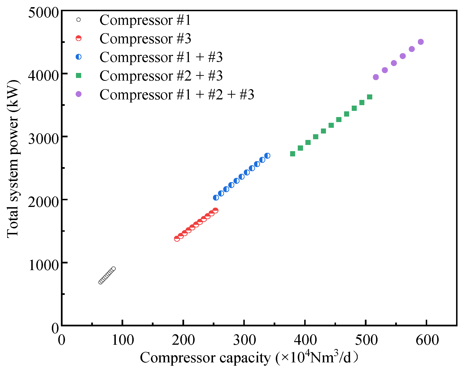
• A multi-objective optimization model based on the NSGA-II algorithm was proposed for the three compressors in the gas storage facility. The objective functions were maximizing gas injection volume and minimizing total energy consumption, with decision variables including compressor and air cooler speeds. Constraints such as compressor operating limits and process requirements were incorporated. The algorithm classified compressor operation conditions into high, medium, and low compression ratios for optimization. The results show that an optimal startup sequence exists: as the daily gas injection volume increases, Compressor #1, #3, and then #2 should be sequentially activated, with parallel operation utilized when necessary to achieve optimal energy efficiency. It was also noted that compressors should avoid operating within certain partial gas injection ranges whenever possible.
• The optimal matching speeds of air coolers and compressors under different conditions and rotational speeds were determined. This study found that reducing the air cooler speed appropriately can significantly save energy while ensuring the maximum outlet temperature requirement for gas injection is met. The energy-saving potential increases as the compression ratio decreases. Under the studied conditions, adjusting air cooler speeds at high compression ratios offers an energy-saving potential of 2%, whereas at low compression ratios, this potential can reach up to 8%.

References

1. Li, Q.; Li, Q.; Wu, J.; Li, X.; Li, H.; Cheng, Y. Wellhead Stability During Development Process of Hydrate Reservoir in the Northern South China Sea: Evolution and Mechanism. Processes 2025, 13, 1630. [Google Scholar] [CrossRef]
2. Li, Q.; Wu, J.; Li, Q.; Wang, F.; Cheng, Y. Sediment Instability Caused by Gas Production from Hydrate-Bearing Sediment in Northern South China Sea by Horizontal Wellbore: Sensitivity Analysis. Nat. Resour. Res. 2025, 34, 1667–1699. [Google Scholar]
3. Ding, G.; Wei, H. Review on 20 years’ UGS construction in China and the prospect. Oil Gas Storage Transp. 2020, 39, 25–31. [Google Scholar]
4. Ma, X.; Zheng, D.; Wei, G.; Ding, G.; Zheng, S. Development directions of major scientific theories and technologies for underground gas storage. Nat. Gas Ind. 2022, 42, 93–99. [Google Scholar]
5. Hong, H.; Jiang, Z.; Ma, W.; Xiong, W.; Zhang, J.; Liu, W.; Wang, Y. Design of an IMCPID Optimized Neural Network for Stepless Flow Control of Reciprocating Mechinery. Appl. Sci. 2021, 11, 7785. [Google Scholar] [CrossRef]
6. Ma, J.; Ding, X.; Horton, W.T.; Ziviani, D. Development of an automated compressor performance mapping using artificial neural network and multiple compressor technologies. Int. J. Refrig. 2020, 120, 66–80. [Google Scholar] [CrossRef]
7. Wang, F.; Li, X.; Chen, X.; Wang, W.; Gong, J. Prediction method for compressor real energy head characteristics based on deep learning network. Oil Gas Storage Transp. 2020, 39, 459–466. [Google Scholar]
8. Chen, J.; Tan, Y. Determination of Optimal Running Scheme about Injection Process of the Natural Gas Storage Reservoirs. Oil Gas Storage Transp. 2002, 06, 3–4+7–10. [Google Scholar]
9. Yang, Y.; Li, S.B.; Chen, Z.W.; Chen, J.W.; Li, P. Optimization measures to maintain economical operation of electrically driven compressor during gas injection in underground gas storage. Nat. Gas Explor. Dev. 2017, 40, 102–106. [Google Scholar]
10. Wu, K.; Tian, Y.; Yang, Y. Optimization of start-up/shutdown scheme of compressor in gas storage period of gas storage at tiered pricing for electricity. Petrochem. Ind. Technol. 2017, 24, 75–77. [Google Scholar]
11. Deb, K.; Pratap, A.; Agarwal, S.; Meyarivan, T. A fast and elitist multiobjective genetic algorithm: NSGA-II. IEEE Trans. Evol. Comput. 2002, 6, 182–197. [Google Scholar] [CrossRef]
12. Wang, A.; Xiao, Y.; Liu, C.; Zhao, Y.; Sun, S. Multi-objective optimization of building energy consumption and thermal comfort based on SVR-NSGA-II. Case Stud. Therm. Eng. 2024, 63, 105368. [Google Scholar] [CrossRef]
13. Ye, L.; Li, C.; Wang, C.; Zheng, J.; Zhong, K.; Wu, T. A multi-objective optimization approach for battery thermal management system based on the combination of BP neural network prediction and NSGA-II algorithm. J. Energy Storage 2024, 99, 113212. [Google Scholar] [CrossRef]
14. Jiang, Q.; Wang, P. NSGA-II algorithm based control parameters optimization strategy for megawatt novel nuclear power systems. Energy 2025, 316, 134444. [Google Scholar] [CrossRef]
15. Huber, M.L.; Lemmon, E.W.; Bell, I.H.; McLinden, M.O. The NIST REFPROP database for highly accurate properties of industrially important fluids. Ind. Eng. Chem. Res. 2022, 61, 15449–15472. [Google Scholar] [CrossRef]
16. Qu, Z. Principle of Reciprocating Compressor; Xi’an Jiaotong University Press: Xi’an, China, 2019. [Google Scholar]
17. Sun, L. Heat Exchanger Process Design; China Petrochemical Press: Beijing, China, 2015. [Google Scholar]
18. Duvenhage, K.; Kröger, D.G. The influence of wind on the performance of forced draught air-cooled heat exchangers. J. Wind. Eng. Ind. Aerodyn. 1996, 62, 259–277. [Google Scholar] [CrossRef]
19. Dong, Z.; Chen, F.; Yu, Y.; Chen, L. Analysis on Relationship between Air Aftercooler Power and Total Power of the Compressor Unit in Long-distance Pipeline Compressor Station. Nat. Gas Oil 2009, 27, 51–54+68. [Google Scholar]
20. Zhang, S.; Yang, W.; Gao, X.; Chen, F. Compressor Station Gas Temperature Circular Rise Simulation and Analysis. Nat. Gas Oil 2019, 37, 36–41. [Google Scholar]
21. Liu, S.; Li, G.; Tong, L.; Xu, Q.; Zhang, J.; Zou, W. Setting program of air cooler in gas compressor stations. Oil Gas Storage Transp. 2019, 38, 228–234. [Google Scholar]
22. Yang, S.; Tao, W. Heat Transfer; Higher Education Press: Beijing, China, 2006. [Google Scholar]
23. Wang, C.; Chi, K. Heat transfer and friction characteristics of plain fin-and-tube heat exchangers, part I: New experimental data. Int. J. Heat Mass Transf. 2000, 43, 2681–2691. [Google Scholar] [CrossRef]
24. Zhou, J.; Peng, J.H.; Luo, S.; Sun, J.H.; Liang, G.C.; Peng, C. Optimization of Gas Injection and Production in Gas Storage Based on Large Depleted Gas Reservoir with Consideration of Safe and Stable Operation. Spec. Oil Gas Reserv. 2021, 28, 76–82. [Google Scholar]
25. Blank, J.; Deb, K. Pymoo: Multi-objective optimization in python. IEEE Access 2020, 8, 89497–89509. [Google Scholar] [CrossRef]
26. Yu, Y.; Sun, S. Compressor Engineering Manual; China Petrochemical Press: Beijing, China, 2012. [Google Scholar]
Figure 1. Sketch of gas injection process at a station in a gas storage reservoir.
Energies 18 03377 g001
Figure 2. Optimization of compressor thermodynamic model calculation flow by GA.
Energies 18 03377 g002
Figure 3. Relationship between wind speed and heat exchanger tube bundle pressure drop.
Energies 18 03377 g003
Figure 4. Air cooler tube bundle heat transfer process: (a) schematic diagram of heat exchange structure; (b) temperature distribution map of hot and cold fluids.
Energies 18 03377 g004
Figure 5. NSGA-II calculation process.
Energies 18 03377 g005
Figure 6. Calculated interstage pressure vs. actual interstage pressure.
Energies 18 03377 g006
Figure 7. Comparison of calculated flow rate with actual flow rate.
Energies 18 03377 g007
Figure 8. Influence of first−stage inlet pressure on compressor capacity.
Energies 18 03377 g008
Figure 9. Effect of different inlet pressures on compressor unit energy consumption.
Energies 18 03377 g009
Figure 10. Influence of first-stage inlet temperature on compressor capacity.
Energies 18 03377 g010
Figure 11. Influence of primary inlet temperature on compressor unit energy consumption.
Energies 18 03377 g011
Figure 12. Influence of second−stage inlet temperature on compressor capacity.
Energies 18 03377 g012
Figure 13. Influence of second−stage inlet temperature on compressor unit energy consumption.
Energies 18 03377 g013
Figure 14. Pareto front plot at high compression ratio.
Energies 18 03377 g014
Figure 15. Pareto frontier plot at medium compression ratio.
Energies 18 03377 g015
Figure 16. Pareto frontier plot at low compression ratio.
Energies 18 03377 g016