1. Introduction
Photovoltaic (PV) panels have become a cornerstone of renewable energy generation, offering a sustainable and environmentally friendly alternative to fossil fuels [
1,
2,
3]. With the growing global demand for clean energy, maximizing the efficiency and reliability of PV systems is more crucial than ever. Advanced methods for controlling and transferring the harvested energy to the grid are essential to ensure seamless integration, reduce losses, and maintain grid stability [
4,
5,
6,
7]. Innovations in control strategies and inverter technologies play a pivotal role in meeting these demands, paving the way for a more resilient and efficient renewable energy infrastructure.
The unequal power generation of different PV modules, caused by partial shading and other PV panel degradation factors such as temperature variations, results in a reduction in overall energy yield, especially when centralized inverters are used [
8,
9]. This scenario is particularly challenging when centralized inverters are applied. On the other hand, as discussed in [
10], the use of distributed microinverters can improve energy harvesting under such conditions. However, this approach increases the overall system complexity due to the large number of inverters operating in parallel. A cost-effective alternative to distributed microinverters is the use of Dual Maximum Power Point Tracking (MPPT) systems, which have proven effective in mitigating partial shading and mismatch losses in photovoltaic (PV) arrays [
11,
12,
13].
Recent research highlights that integrating advanced control algorithms with dual MPPT systems not only enhances power extraction but also improves inverter reliability [
14,
15,
16] and the power quality indicators in the grid side. Dual MPPT systems have been implemented in various applications, such as the efficiency optimization of a DSP-based standalone PV system [
17], a dual-discrete model predictive control-based MPPT for PV systems [
18], and a novel dual MPPT control strategy for wind generators [
19].
The two-level VSI (2L-VSI) grid-tied topology is commonly used to interface the PV arrays with the AC grid; however, it suffers from high electrical stress and harmonics. On the other hand, multi-level inverters are able to produce current waveforms with low harmonic distortion and reduced switching losses. Today, many three-level VSI (3L-VSI) topologies have been extensively discussed in the literature, such as the neutral-point-clamped (NPC) VSI, flying-capacitor VSI, and cascaded H-bridge VSI. However, especially when low-voltage applications are considered, such as the case of commercial dual MPPT converters, the T-Type Three-Level Three-Phase inverter (3L T-Type VSI) becomes an interesting alternative, since it combines the positive aspects of the two-level converter—such as low conduction losses, small part count, and a simple operation principle—with the advantages of the three-level converter, such as low switching losses and superior output current quality [
20]. The 3L T-Type VSI can reduce six power diodes in comparison to the 3L-NPC VSI, while maintaining reduced harmonic distortion and better thermal performance [
21], as well as reducing the common-mode voltage [
15,
22,
23].
The intrinsic characteristic of the 3L T-Type VSI of splitting capacitors is suitable for the straightforward integration of dual MPPT PV systems consisting of two independent PV string arrays, since each array can be direct connected to each 3L T-Type VSI’s DC-link capacitors. This kind of implementation has not been reported in the literature yet and represents an original contribution of the present work.
However, the connection of independent MPPT converters to each DC-link capacitor raises the problem of capacitor voltage balance [
24,
25,
26], the solution to which is considered in this paper. Nevertheless, using standard methods for DC-link capacitor balance has some impact on the output current waveform, since the common balancing methods consist of summing a controlled DC signal to the PWM references.
Therefore, to improve the output current waveform produced by the 3L T-Type VSI, the sliding mode control (SMC) technique is implemented, since it is well known to yield a low distortion current [
27]. This effect of the SMC is further magnified by the low distortion characteristic of the 3L T-Type topology discussed above.
It is worth highlighting that SMC has gained widespread adoption in renewable energy and photovoltaic (PV) systems due to its robustness against parameter variations and external disturbances. Recent advancements include enhancing solar PV panel efficiency using double-integral sliding mode MPPT control [
28] and employing SMC for the control of boost converters in PV systems [
29]. In [
27], a proportional–integral (PI) and an SMC controller were applied in the three-phase grid-tied 3L T-Type quasi-Z-source inverter with an LCL filter.
An adaptive dynamic surface sliding mode control strategy is proposed in [
30] to enhance energy extraction from photovoltaic panels while mitigating current and voltage fluctuations caused by irradiance variations. Although the simulation results are promising, the study does not provide Hardware-In-the-Loop (HIL) validation or experimental verification. Similarly, Ref. [
31] proposed a generalized sliding mode control technique with adaptive gain scheduling to enhance the convergence speed of the grid current and to improve overshoot and steady-state performance in a three-phase, two-level inverter. In [
32], a fuzzy controller was deployed to dynamically adjust the SMC gains, aiming to provide a fast transient response with reduced overshoot and improved steady-state performance. In [
33], a robust SMC based on the PV power curve was proposed to control a single-phase, single-stage, quasi Z-source inverter connected to the utility grid.
In [
34], a voltage controller based on SMC was investigated, leveraging its disturbance observer capability to enhance robustness and eliminate current sensors. Furthermore, Ref. [
35] proposes an improved disturbance observer based on fixed-time SMC and an optimal state observer for standalone 3L T-Type inverters; however, focus is given to state observer performance, to the detriment of enhancing the SMC technique.
In the aforementioned works, the Perturb and Observe (P&O) MPPT method was employed in a classical PV integrated grid that suffered from steady-state oscillations under rapidly changing irradiance conditions. Therefore, applying an enhanced nonlinear SMC alongside the Notable P&O observer not only enhances the whole system’s robustness but also helps the DC side regulate faster under dynamic changes.
Based on the discussion above, and to the best of the authors’ knowledge, the integration of dual MPPT systems with 3L T-Type inverters represents an unexplored area in the literature. Therefore, this paper aims to bridge this gap by introducing an enhanced SMC strategy leveraging a super-twisting control algorithm to overcome the limitations of traditional SMC, which are specifically high chattering and discontinuous control input, by effectively mitigating the intrinsic chattering of the conventional SMC while maintaining independence between the two DC inputs and simultaneously ensuring high dynamic performance. Furthermore, by integrating an enhanced nonlinear sliding mode controller with the Perturb and Observe (P&O) MPPT algorithm, the steady-state oscillations commonly observed in the aforementioned approaches under rapidly changing irradiance conditions are effectively mitigated by the proposed method.
This novel approach not only optimizes power extraction from dual PV arrays but also provides stable and efficient grid power injection under varying operating conditions. In this paper, a comprehensive design and analysis of the proposed control strategy are provided, supported by detailed real-time simulations based on the Hardware-In-the-Loop platform Opal-RT. The results demonstrate its potential to advance the state of the art in PV system control, under various abnormal grid conditions, paving the way for robust, high-performance solutions in modern solar energy systems. In contrast to recent publications on PV integrated inverters that focus on system modeling [
36] or the development of disturbance observers to reduce steady-state error and improve dynamic response, the proposed method is model-independent and demonstrates strong robustness under uncertainties such as parameter variations.
The main contributions of this paper are summarized below:
Proposal of an architecture that directly connects two independent PV arrays to the split DC-link capacitors of a 3L T-Type inverter, enabling a compact and efficient configuration not previously addressed in the literature.
An enhanced sliding mode control strategy based on the super-twisting algorithm is developed specifically for the proposed topology to improve the current quality and eliminate high-frequency chattering while maintaining independent control of each MPPT channel.
A comprehensive design and real-time Hardware-in-the-Loop (HIL) simulation using the Opal-RT platform to validate the performance and robustness of the proposed system are introduced, which are tested under various grid disturbances and parameter variations.
The rest of this paper is organized as follows:
Section 2 presents the modeling of the power converter, while the control design considering the DC-side MPPT controller, AC-side SMC controller, and the strategy used to avoid voltage mismatch between the split DC-link capacitors are discussed in
Section 3. The effectiveness of the overall control strategy for the grid-tied dual MPPT with 3L T-Type inverter is demonstrated through real-time HIL results discussed in
Section 4. Finally, in
Section 5, the main achievements and conclusions are presented.
3. Controller Design
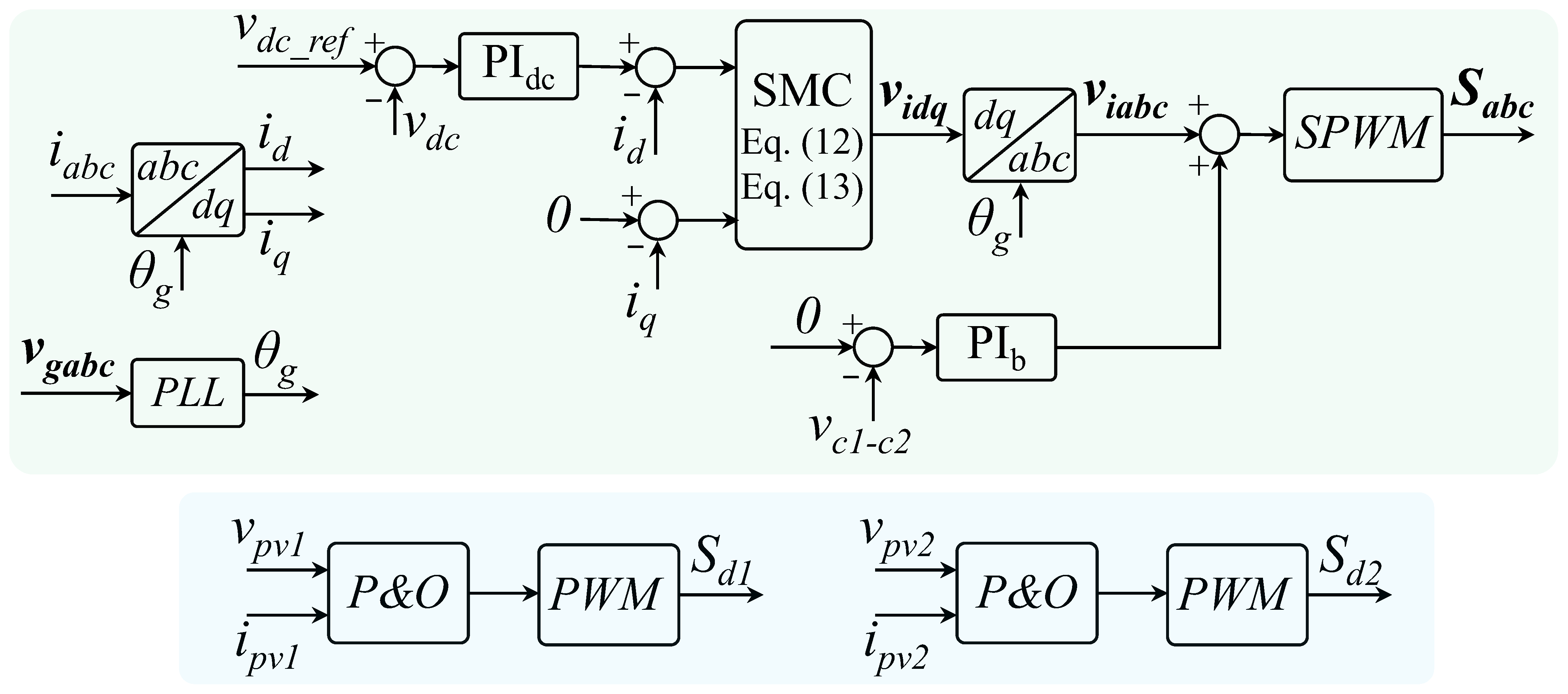
The design of the control framework ensures optimal system performance by managing the DC and AC sides of the energy conversion process. This section elaborates on the methodologies used to achieve these objectives according to the general control architecture shown in
Figure 2.
The DC-side control is designed to maximize power extraction from the solar panels and regulate the output voltage of the boost converters. By leveraging the Perturb and Observe method, the control dynamically adjusts the duty cycle of each boost converter to extract maximum power under varying environmental conditions. The output voltage regulation aligns with the broader control strategy, ensuring seamless integration with the AC-side control.
The AC-side control focuses on ensuring efficient and accurate power transfer into the grid. It employs a dual-loop structure: the first is a slow dynamic loop that regulates the DC-link voltage of the T-type inverter, while the second loop governs the sinusoidal current injection into the grid, presenting a fast transient response. By representing the system equations from the natural abc reference frame to the synchronous reference frame (dq reference frame) using Park transformation, the control design is greatly simplified. Within this transformed frame, the sliding mode control method regulates the direct (d) and quadrature (q) components of the inverter’s output current. An overview of the control strategy discussed in this work is shown in
Figure 2.
Lastly, a third controller is used to ensure that the voltage across the DC-link split capacitors of the 3L T-Type VSI is balanced. Nevertheless, this controller exhibits negligible influence over the performance of the conventional dual-loop strategy discussed above. This comprehensive control strategy, summarized in
Figure 2, enables the system to adapt effectively to dynamic conditions, ensuring optimal energy utilization and reliable grid operation.
3.1. DC-Side Control
The DC-side control consists of two primary components: The first component focuses on extracting maximum power from the solar panels. Each panel exhibits distinct photovoltaic (PV) characteristics that determine the maximum power that it can generate under specific irradiation and temperature conditions. Using the Perturb and Observe method proposed in [
37], the control strategy ensures maximum power extraction by dynamically adjusting the duty cycle applied to the switch of each boost converter.
The second component, which manages the output voltage control of each boost converter, is integrated into the AC-side control framework as shown in the block diagram of
Figure 2. This aspect of the control methodology will be detailed in the subsequent chapter.
The d-axis reference current
determines the power transfer between the PV arrays and the grid, which is derived based on the DC-link voltage of the 3L T-Type inverter. The power balance between the input power in the DC link and the grid is ensured if the DC-link voltage is maintained and regulated at the reference value
. If there is a surplus of power being injected by the PV arrays, the DC-link voltage tends to increase, and the PI controller will increase the value of
, increasing the output power injected into the grid and leading to a decrease in the DC-link voltage. The reference current
is given by
Since the main aim of PV inverters is to transfer the real power to the grid and operate with a unitary power factor, the current reference is set to zero.
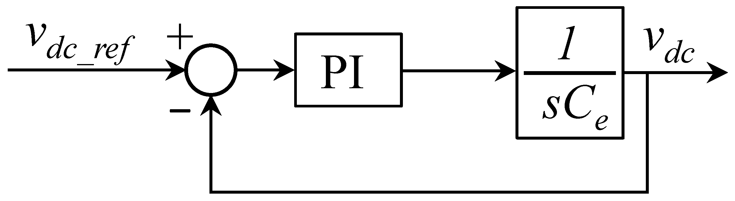
The DC-link voltage controller is modeled as shown in the block diagram of
Figure 3, obtained by using a small-signal analysis [
38]; it establishes a relationship between the DC-link voltage,
, and the current at the inverter output, i.e., the current control variable
, as discussed in the previous section.
Since the DC-link voltage control is expected to exhibit a slower dynamic response in order to avoid interaction with the fast current controller, it is tuned considering the damping factor
and the desired natural oscillation frequency
. Based on these parameters and on the value of the DC-link capacitor (
), the following equations can be used to estimate the proportional
) and integral (
) gains of the DC voltage controller, as given by Equations (6) and (7). Note that from the DC-link voltage controller perspective, the total capacitance consists of the series connection of
and
; since these capacitors have the same values, it results in
:
Although direct measurement of the total DC-link voltage
is commonly required for voltage regulation, in the proposed control architecture this measurement can be effectively avoided. Given that the individual voltages across the split capacitors
and
are already sensed for implementing the auxiliary control loop that will be introduced in
Section 3.5, the total DC-link voltage can be accurately reconstructed in real time by summing the voltages of the split capacitors, as expressed in Equation (1). This strategy reduces the number of required voltage sensors, thereby simplifying the hardware implementation without degrading the control performance.
3.2. Grid Current Control
The AC-side current control focuses on ensuring the injection of sinusoidal current into the grid. The control strategy employs two interconnected loops. The first loop regulates the DC-side input voltage of the T-Type inverter, while the second loop controls the current injected into the grid.
As discussed above, for the sake of simplicity, the control of the grid current is performed using a sliding mode controller implemented using the synchronous reference frame. Therefore, applying the Park transformation to Equation (4) results in Equations (8) and (9) considering the orthogonal
and
axes of the synchronous reference frame, respectively:
where the subscripts
and
represent the direct and quadrature components, respectively, and
is the frequency of the grid.
Then, based on Equations (8) and (9), the sliding functions for the SMC approach are defined in Equations (10) and (11) considering the primary objective of current reference tracking in the
dq frame. The reference value for the
current is given by
, while
denotes the reference value for
.
The super-twisting control law is expressed as follows:
where
,
,
, and
are the positive gains of the reaching law, which determine the behavior of the controller and are tuned based on system dynamics. It can be observed from the reaching laws defined in Equations (12) and (13) that, although the proposed SMC law is a second-order sliding mode control method, it requires only the sliding function and not its derivative. On the other hand, it provides finite-time convergence to the sliding surface and ensures robustness against matched uncertainties and disturbances.
The derivative of the sliding surfaces (
and
) yields
where
and
are defined as follows:
The terms
and
are treated as bounded uncertainties subject to fluctuations and can be expressed as follows:
3.3. Stability Analysis of the Grid Current Controller
To ensure the stability of the current controller under the proposed control scheme, the following Lyapunov functions are considered for both the
- and
-axis reference frames:
where
= 2/3, as proposed in [
39]; 0.5
and
are the quadratic energy terms to monitor the sliding surface;
and
are power terms to handle the internal dynamics of the controller; and finally,
and
are the integral terms of the SMC reaching law and defined as follows:
To verify the satisfaction of the Lyapunov stability criterion, the time derivatives of the Lyapunov functions along the system trajectories in both the
- and
-axis reference frames must be negative-definite, as shown below:
By substituting Equations (12)–(15) into Equations (24) and (25), the following expressions are obtained:
Considering the worst-case arrangement of the sign terms is employed, the derivatives of Equations (26) and (27) become
Assuming
,
, Equations (28) and (29) can be rewritten as follows:
In order to ensure that the Lyapunov function in both the
- and
-axes is decreasing, the conditions specified in Equations (28) and (29) must be satisfied. Assuming
, and
, the SMC gains can be defined by the inequalities of Equations (32) and (33), providing finite-time stability of the closed-loop system under the action of the SMC.
If the parameters are selected exactly as specified in Equations (32) and (33), the Lyapunov functions are strictly decreasing for all sliding functions, rather than zero. However, if the parameters are not exactly equal to the mentioned terms but are instead chosen to be sufficiently larger, the damping terms
and
found in Equation (28), along with the damping terms
and
of Equation (29), are sufficiently greater than the terms
,
,
, and
, thereby ensuring their dominance in the overall dynamic behavior. Hence, the analysis of the sliding surfaces derivatives is simplified to
Given that the terms and are always positive values, the Lyapunov functions decrease in finite time; hence, the origin is finite-time stable.
3.4. Parameter Selection in SMC Reaching Law
The tuning of the SMC coefficients depends on the bounds of the system’s uncertainties. According to the Lyapunov-based analysis carried out in the last section, the gains must satisfy Equations (34) and (35) to guarantee the robustness and stability of the system. If the assumptions are reframed as
due to the strong feature of the super-twisting SMC method in chattering reduction, Equations (34) and (35) can be rewritten as follows:
where
and
represents the bounds of the uncertainties in the derivative of the sliding variable
reflects the chattering magnitude and influences the selection of the control parameters.
Notably, there is an inverse relationship between and the gains and , which makes the tuning particularly challenging. While increasing the gains enhances the stability margin and guarantees the satisfaction of the Lyapunov function, it may also reduce the effectiveness of chattering mitigation. Therefore, selecting optimal values for and requires a careful balance between stability and chattering suppression, typically achieved through detailed simulations. Nevertheless, these bounds only show the minimum required values for the parameters that guarantee the system’s stability, while the optimized values are defined based on the empirical and iterative tuning. For the iterative tuning, the robustness and stability of the system are the first goal. The tuning process starts from the best values for the parameters to make the system robust and stable. Then, the values of and are gradually adjusted to reduce the chattering. The coefficients and are adjusted afterwards to manage the integral action for overshoot and smoothness.
3.5. Split Capacitors’ Voltage Balance Control
The connection of independent MPPT converters to each DC-link capacitor raises the problem of capacitors’ voltage balance. Given that the DC-DC converter used to implement the dual MPPT functionality is based on the boost topology, any significant imbalance between the capacitor voltages could lead to a situation in which one of the capacitor voltages exceeds the corresponding PV array voltage. This condition would inhibit effective power transfer from the photovoltaic modules to the DC link.
Many approaches have been proposed in the literature to solve the intrinsic problem of DC voltage imbalance that affects the 3L T-Type inverter. In this work, we applied a simple method based on summing a controlled DC signal to the modulating signal of the PWM [
25]. The technique consists of calculating the difference between the split capacitors’ voltages, i.e.,
and
—see Equation (32)—and applying this error to a PI controller, as shown in the simplified block diagram of
Figure 4.
This controller is designed in a similar form to the PI controller discussed in
Section 3.1. However, unlike that approach, the DC-link capacitors are series-connected, and
, changing the design equations to
It should be highlighted that the effect of the individual DC-link capacitor voltage balancing may conflict with the
control loop discussed in
Section 3.1, which determines the current reference
. To avoid interactions between these two control loops, the voltage-balancing loop (
Figure 4) is tuned to exhibit a slower dynamic response than the control loop presented in
Figure 3. In this work, it is proposed that the natural oscillation frequency of the capacitor’s voltage-balancing loop, denoted as
, be set one decade lower than the natural frequency of the DC-link voltage control loop of
Section 3.1, i.e.,
.
4. Real-Time Evaluation and Results
The effectiveness of the enhanced sliding mode control method presented in the previous sections was validated through real-time simulation of the dual MPPT systems integrated with Three-Level T-Type PV Inverters, as depicted in
Figure 1. The system parameters are listed in
Table 2. The simulations were conducted using the Opal-RT OP5600 Hardware-in-the-Loop (HIL) platform, following a predefined sequence of programmed events designed to highlight the key characteristics of the proposed grid-tied inverter.
4.1. Real-Time Simulation Workflow
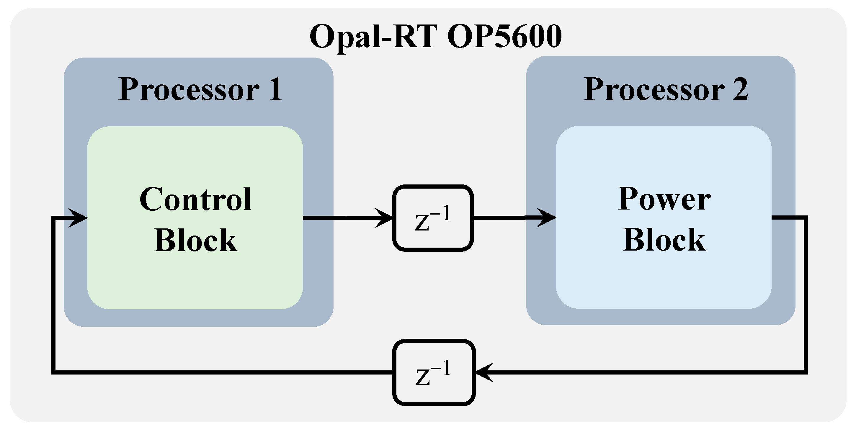
The workflow for generating the real-time results is illustrated in
Figure 5. The real-time simulation approach employed in this study is based on the Software-in-the-Loop (SIL) concept, enabling rapid prototyping of the controllers. The linear PI controllers were implemented using MATLAB/Simulink control blocks, while the sliding mode controller was integrated through an S-function block.
The power stage, consisting of the power converter, output inductive filter, PV panels, and the main grid, was modeled within the power block, as shown in
Figure 5. To accurately replicate the behavior of a DSP-based control implementation, all measurements transferred from the power block to the control block were delayed by one sampling step. Similarly, a one-step delay was introduced in the control signals transmitted from the control block to the power block. While this delay mimics the real-world conditions of experimental implementations, it is also a fundamental requirement to ensure proper data exchange between the power and control blocks. This is necessary because each block operates on a separate microprocessor within the Opal-RT OP5600 hardware, effectively decoupling the power and control sections, similar to conventional experimental setups.
Before deployment, both the control and power models underwent offline validation through MATLAB/Simulink simulations. Subsequently, they were compiled using the RT-Lab software, version 2022, provided by Opal-RT, generating two distinct real-time execution codes—one for the control block and another for the power block. These codes were then uploaded onto separate microprocessors within the OP5600 hardware to ensure independent execution.
Finally, the output waveforms generated by the HIL platform were acquired using an oscilloscope. The results obtained for each test scenario are presented and analyzed in detail in the following subsections, providing a comprehensive evaluation of the proposed control strategy’s performance.
4.2. Real-Time Performance Assessment Test Cases
The simulation results were structured to emphasize the key characteristics of the proposed control approach under both steady-state and transient conditions. The analysis focused on critical performance indicators, considering AC-side parameters such as the total harmonic distortion of current (THDi), settling time (), and power factor (PF). Additionally, DC-side parameters were evaluated, including DC-link voltage ripple, settling time, and voltage balance between the two input ports ( and ).
To assess the effectiveness of the proposed controller and validate its practical applicability, a series of real-world test cases were conducted, as detailed below. This structured evaluation provides a comprehensive assessment of the controller’s dynamic and steady-state performance under realistic operating conditions:
Test Case A: DC-link voltage reference step change;
Test Case B: Step change in irradiance;
Test Case C: Shadowing effect with independent irradiance variations at each MPPT input;
Test Case D: Grid voltage sag and swell;
Test Case E: Grid voltage distortion;
Test Case F: Sensitivity to parameter variations.
4.2.1. DC-Link Voltage Disturbance
In order to validate the design of the DC-link voltage controller, a DC voltage reference step is shown in
Figure 6. The controller is able to achieve a steady state in less than one grid cycle, with a settling time of 15 ms and overshot of 5%, showing fast disturbance rejection. A detailed view DC-link voltage and its reference signal are shown in
Figure 7, as well as the current in phase
a superimposed onto the current reference.
4.2.2. Effect of Temperature Variation
The sensitivity of the proposed control approach considering variations in the temperature of the PV array cells is depicted in
Figure 8. The solar cells that compose each of the PV arrays were subjected to a step-up temperature variation from 25 °C to 45 °C. Although this condition is uncommon in practical applications due to the low dynamics of the temperature, it represents a worst-case scenario that is interesting for assessing the performance of the controller. The sudden change in temperature leads to a decrease in the power generated by the PVs, thereby reducing the current injected into the grid. Before the temperature change, the power injected into the grid was 15.74 kW, with a power factor of 0.999. During the temperature increase and consequently current reduction, the power injected into the grid decreased to 14.8 kW; however, the power factor remained unchanged. The balance of the DC link was ensured by the external control loop, and the THD of the current remained at 4.5%.
4.2.3. Effect of Irradiance Variation
Figure 9 shows the DC-link voltage (
), the voltage in both of the DC-link capacitors (
and
), and the grid currents for phases
a and
b considering a step change in the overall irradiance seen by the PVs from 1000 W/m
2 to 500 W/m
2. The DC-link voltage controller was able to rapidly track (
= 15 ms) the reference voltage with 5% overshoot, demonstrating the robustness of the proposed approach against setting-point variations and intermittency of the renewable source. As expected, changes in irradiation resulted in a displacement of the maximum power point, thereby reducing the active power injected into the grid from 15.74 kW to 8.4 kW. This is reflected in the current waveforms, which decreased during the irradiance step.
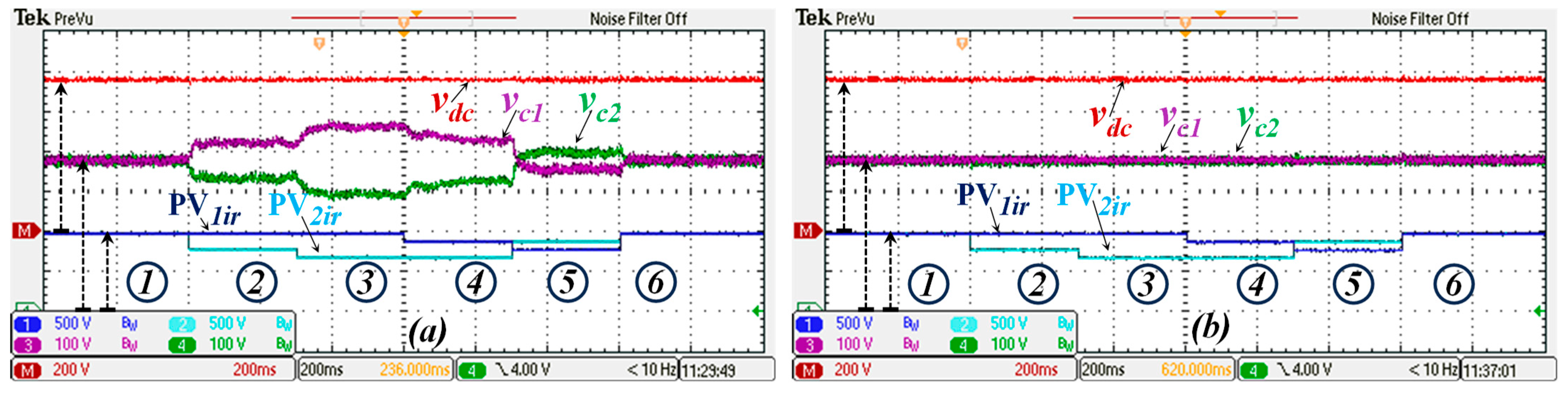
4.2.4. Shadowing Condition
Shadowing is a common and highly probable condition in real-world MPPT inverter applications. To assess its impact on the proposed dual-MPPT 3L T-Type grid-tied inverter with MSC control, various shadowing scenarios were tested. These conditions resulted in different irradiance levels across the PV groups connected to each input port, as detailed in
Table 3 for the six stages highlighted in
Figure 10.
The results presented in
Figure 10a demonstrate the behavior of the voltage across the split capacitors if the voltage balance control was not deployed. In step 3, in which the difference in irradiance between the two PV groups was higher (300 W/m
2), the voltage across the second DC-link capacitor
reached 300 V, whilst the voltage
was 450 V. The active power flowing into the grid and the power factor index are highlighted in
Table 3 for each of the irradiance conditions.
On the other hand,
Figure 10b shows the behavior of the DC voltages when the balancing controller is activated. It should be noted that even for the highest irradiance difference between the PV arrays, the DC voltage remains balanced. In this case, the voltage rating of the switches at the midpoint of the 3L T-Type VSI shown in
Figure 1 is half the DC-link voltage, since the split capacitors’ voltage balance is ensured. In addition, as shown in
Table 3, the unitary power factor is maintained for any irradiance condition.
4.2.5. Grid Voltage Sag and Swell
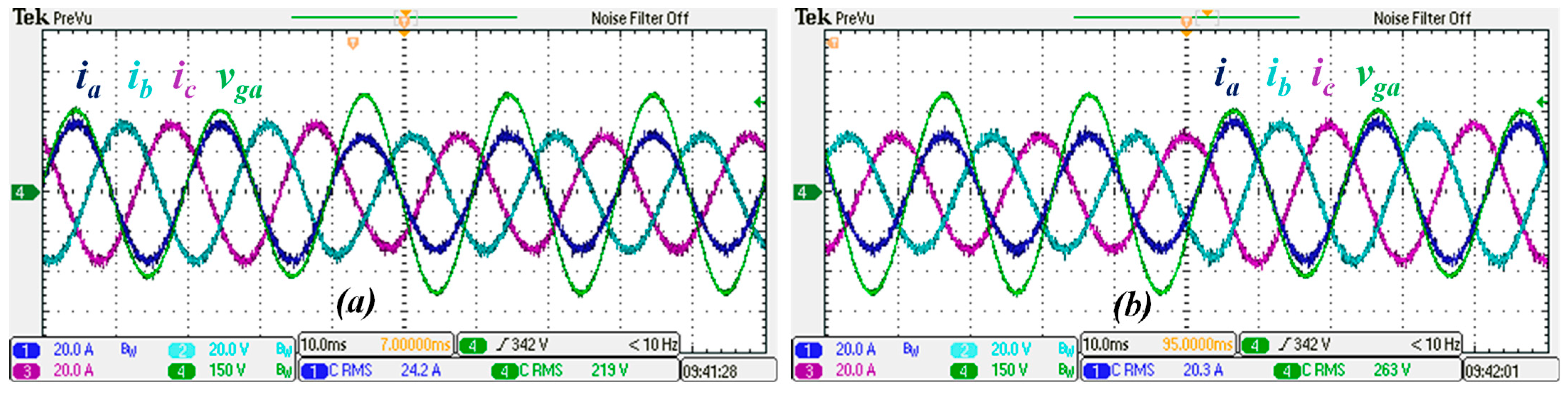
The robustness of the proposed system considering non-ideal grid conditions was evaluated considering two additional scenarios in which sudden changes were introduced in the grid voltage. The voltage sags and swells could be caused by grid faults or due to sudden changes in load or generated power flowing through the main grid. The first scenario consists of a voltage sag of 40%, i.e., the phase-to-neutral grid voltage experiences a sudden drop from 220 V rms to 132 V rms. The grid currents during the voltage sag are shown in
Figure 11, along with the voltage in phase a (
), where it can be seen that the currents take approximately half a cycle to achieve a steady state.
An additional and particularly challenging scenario is illustrated in
Figure 12, showing a 20% voltage swell. The grid voltage was intentionally increased to an unusually high level to evaluate the controller’s performance, considering the maximum overvoltage tolerance. According to IEEE Std. 1547-2018 [
40], grid-tied inverters must withstand overvoltage up to 20% of the nominal grid voltage. For voltages exceeding this threshold, the inverter must be disconnected from the grid. Despite this extreme condition, the current waveforms maintain high quality, while the amplitude is reduced to ensure constant power injection into the grid. During the events of voltage sag and swell, the power injected into the grid remained constant at 15.75 kW, along with the power factor of 0.999.
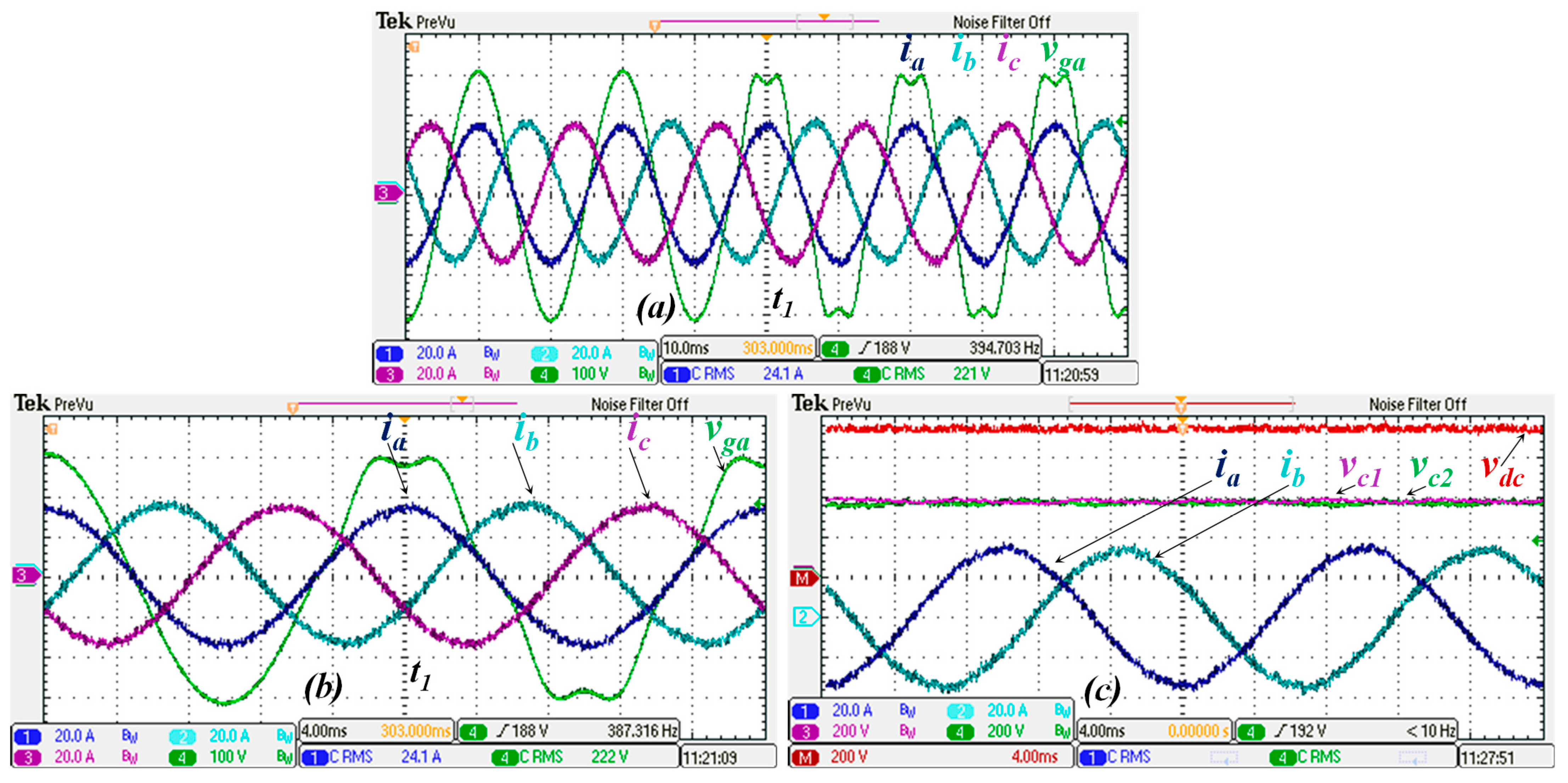
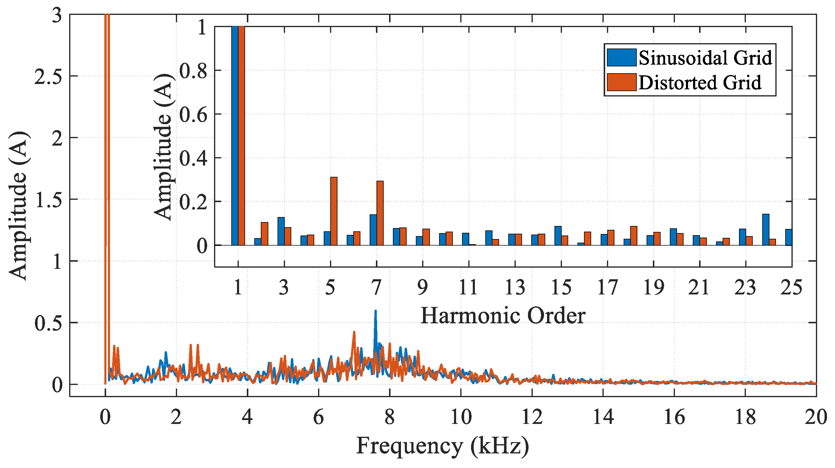
4.2.6. Grid Voltage Distortion
Inverters with the rated power discussed in this work are commonly used in residential and commercial buildings, environments often dominated by nonlinear loads that cause voltage distortions due to the interaction of harmonic currents with the grid impedance. Therefore, it is important to ensure that the inverters can handle distorted voltage. A representative test case was implemented considering 10% of the fifth harmonic component superimposed on the grid voltage, as shown in
Figure 13. The inverter’s output current exhibits low sensitivity to the grid voltage, since a positive sequence PLL is used to extract the fundamental component of the grid voltage, which is used to generate the current reference along with the error of the
voltage processed by the PI controller, as depicted in the control block diagram shown in
Figure 1.
Without any distortion in the grid voltage, the ripple of
is 21 V peak-to-peak. Otherwise, the fifth harmonic increases the
ripple to 28 V. However, the practical effect on the grid current waveform is negligible, as shown in
Figure 13b and in the spectra shown in
Figure 14. The amplitude of the fundamental current component is 34 A, while the amplitude of the fifth harmonic is 0.31 A, representing 0.9% distortion for this specific harmonic. The overall THDi is 4.5% in the event that the grid voltage is sinusoidal, while it is 4.8% for distorted grid voltage.
4.2.7. Parameters’ Sensitivity
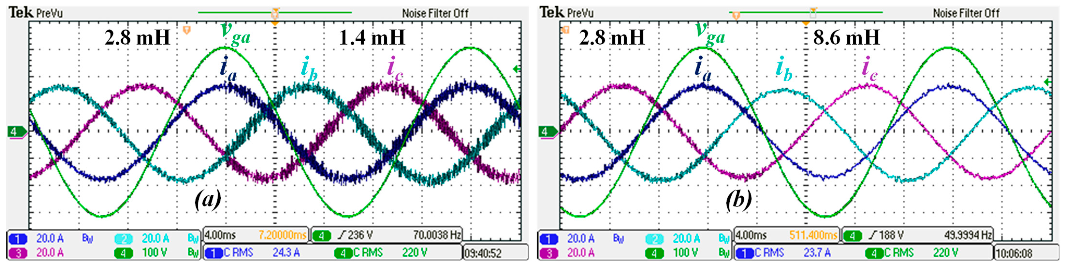
Finally, the SMC is widely recognized for its simple implementation, fast dynamic response, and robustness against parameter uncertainties. This work evaluates these attributes by analyzing variations in the output filter inductance, which may occur due to aging, heating, or imprecise manufacturing processes. Additionally, since the grid inductance is typically unknown, it effectively adds to the total filter inductance.
Figure 15a illustrates the grid current waveforms when the filter inductance is reduced to half of its nominal value, decreasing from 2.8 mH to 1.4 mH. As expected, this reduction increases the current ripple and degrades THDi from 4.5% to 9%. On the other hand, when the nominal output filter inductance is increased threefold, from 2.8 mH to 8.4 mH (see
Figure 15b), the current waveform improves, reflecting a reduced ripple and lower THDi of 2.5%.
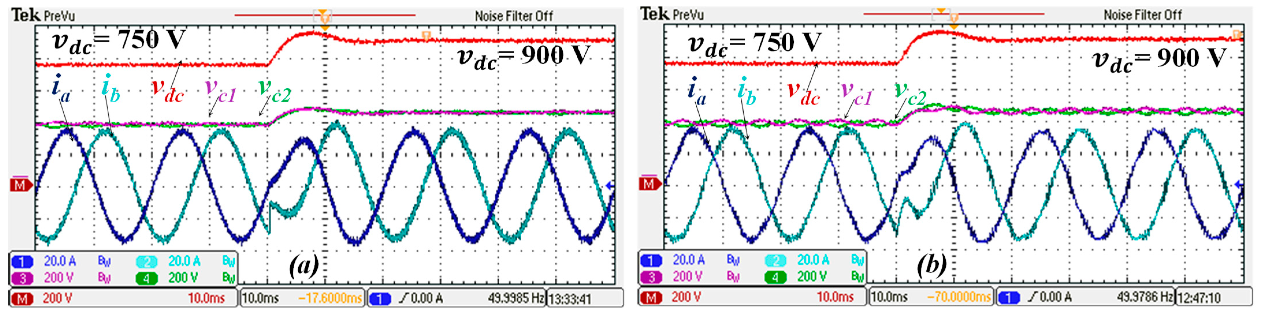
4.2.8. Comparison of Proposed SMC with Conventional PI Controller
Linear current control of power inverters is a well-known approach, especially considering proportional–integral (PI) controllers in the synchronous reference frame. In this section, a comprehensive comparative analysis is performed between the proposed SMC and the conventional PI controller. The parameters of the system are presented in
Table 2 and are the same for both controllers. The control architecture is the one presented in
Figure 1, with the SMC block replaced by PI controllers.
Th PI current controller is designed based on the desired crossover frequency (
) of the current loop [
1] and the desired phase margin (
), aiming to regulate the
dq-frame currents. Therefore, the gains of the current PI controller can be designed according to Equation s (41) and (42). Considering the crossover frequency sevenfold below the switching frequency (700 Hz) and the desired phase margin of 60°, the PI gains are obtained as
= 0.1 and
= 7.0.
The comparison of SMC- and PI-controlled systems is presented in
Figure 16 and
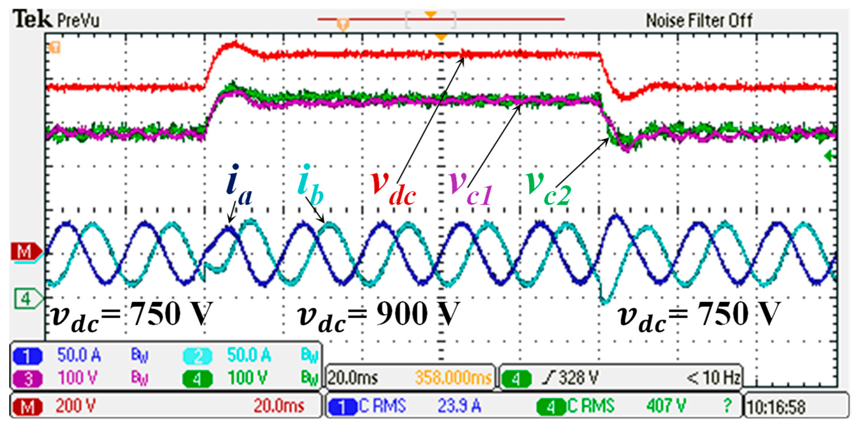
Figure 17. A step change in the DC-link voltage reference from 750 V to 900 V is presented in
Figure 16. The transient response, specifically the settling time and overshoot, is similar for both approaches, as presented in
Table 4. The current THD is lower for the SMC controller (4.5%) than for the PI controller (6%). However, the ripple seen in the voltage of the split capacitors is remarkably high for the PI controller (45 V), whilst it is 20 V for the SMC. The higher DC-voltage ripple of the PI controller approach results in a higher fifth-harmonic current distortion of 3%, as seen in
Figure 18, whilst this specific component shows a negligible value for the SMC. The power factor is the same for both approaches.
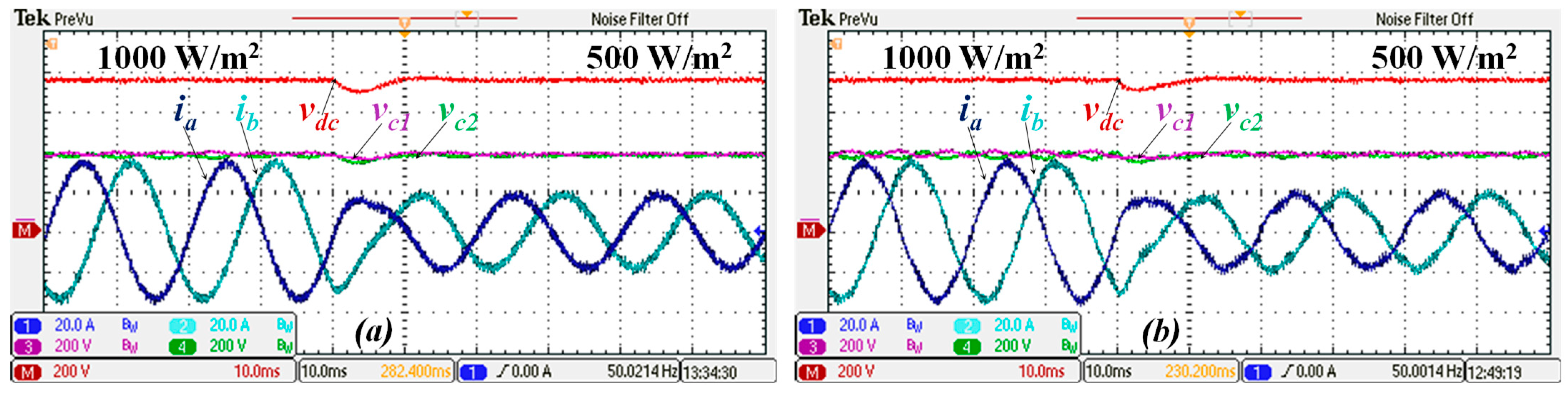
Figure 17 shows the behavior of both approaches for a step variation in irradiance from 1000 W/m
2 to 500 W/m
2. When the irradiance is half the initial value, the power injected into the grid decreases, as does the amplitude of the injected current, resulting in an increase in THD values, which is verified for both approaches.
Therefore, in spite of the similarity between the two approaches, the proposed SMC controller yields a slightly higher current quality and lower ripple.
5. Conclusions
Dual Maximum Power Point Tracking (MPPT) inverters play a crucial role in residential and small commercial solar power systems by optimizing energy extraction from two independent photovoltaic arrays, thereby enhancing overall efficiency and energy yield. In this work, an enhanced sliding mode control (SMC) strategy was proposed, specifically designed for dual MPPT and Three-Level T-Type PV inverters.
This approach integrates the simplicity of conventional PI controllers with the superior robustness and dynamic performance of sliding mode control, ensuring reliable operation under varying conditions. The combination of conventional MPPT with the advanced SMC-based AC-side control results in improved dynamic response, higher power quality, and increased robustness under realistic operating conditions. The proposed control strategy was validated through HIL real-time simulations, leveraging the Software-In-the-Loop (SIL) concept, where the controller is implemented directly within the HIL system. The performance of the dual MPPT Three-Level inverter and the proposed SMC was extensively tested under various scenarios, including normal and abnormal grid voltage conditions, sudden irradiance changes at each MPPT input, and significant parameter variations to assess robustness.
The results demonstrate that the inverter’s output current and DC-link voltages exhibit a fast transient response. In the presence of perturbations in the DC link and variations in irradiance, the steady-state condition was reached within 15 ms, with an overshoot of less than 5%. In steady-state operation, the current THD complied with international standards, as defined by IEEE Std. 519 [
41] and IEC 61000-2-2 [
42]. The current THD was maintained below 4.8%, even under highly distorted grid voltage conditions. The controller effectively maintained active power injection into the grid even under fault conditions or abnormal voltage levels, while also sustaining a unity power factor throughout these conditions, further validating its robustness and reliability.
Despite the simplicity of real-time implementation, the tuning of the control gains in the proposed SMC technique remains nontrivial, particularly when extended to more complex power converter topologies. Therefore, several challenges persist, especially concerning the scalability of the method to advanced converter architectures. For instance, future work may explore the extension of the control strategy to systems incorporating higher-order passive filters, such as LCL filters in Three-Level T-Type inverters, or its application to modular multi-level converters (MMCs), which present additional control and stability complexities. Furthermore, while the present study focuses on a PV inverter operating in a grid-following mode, the proposed control strategy could be extended to voltage-controlled grid-forming or standalone configurations. These directions, along with the experimental validation of the proposed technique on a hardware prototype under realistic operating conditions (such as noise, measurement uncertainties, and switching non-idealities), represent important areas for future investigation. Finally, a detailed performance assessment of the proposed architecture could be conducted in comparison with conventional two-level voltage source inverters commonly employed in micro and mini distributed generation systems.


 ,
, 


