Abstract
As urban populations grow and energy demands escalate, it is increasingly challenging for existing building electrical infrastructure in densely populated areas to meet contemporary energy requirements. Traditional grid expansion methods often impose prohibitive economic costs and environmental impacts. Photovoltaic-battery (PVB) systems emerge as a sustainable alternative to enhance building energy self-sufficiency while addressing transformer capacity constraints. This study develops a multi-objective optimization methodology for PVB system configuration in retrofit applications, introducing the transmission limit ratio (TLR) metric to quantify grid interaction capacity. Taking a residential building as a case study, the constraints on configuration variables under insufficient transformer capacity are obtained through simulation. Applying the NSGA-II algorithm, optimal configurations are identified for economic and environmental scenarios. In terms of configuration, a PVB system, 0.743 PV penetration, 205 kWh battery is the best optimal configuration for an economic operation scenario, while 1.356 PV penetration and 201 kWh battery is the best for an environmental operation scenario, when the TLR is 0.8. The analysis demonstrates PV penetration’s critical role in scenario transition, while battery capacity primarily ensures system stability across TLR variations. This methodology provides practical insights for engineers in optimizing sustainable energy systems within existing infrastructure constraints, particularly relevant for high-density urban environments.
1. Introduction
Due to rapid population growth and urbanization [1], the energy crisis has become increasingly severe, with energy demand reaching unprecedented levels [2]. Consequently, increased energy consumption has amplified carbon emissions, creating urgent challenges for sustainable urban development [3]. The 2024 Statistical Review of World Energy reports that energy-related emissions exceeded the 40 GtCO2e level, with emissions from direct use of energy reaching 35 GtCO2e for the first time ever [4]. The building sector plays a pivotal role in this dilemma, due to its high energy usage and environmental impact [5,6]. Notably, energy consumption in this sector accounts for 36% of the global energy demand and contributes to 39% of global CO2 emissions [7,8].
To address these challenges, it is crucial to decrease fossil fuel dependence and actively stimulate the transition to renewable energy sources [9]. This transition holds particular significance for the cities where rapid urbanization coincides with evolving energy infrastructure. Renewable energy has immense significance in enhancing energy structures, safeguarding the ecological environment, combating the repercussions of climate change, and fostering sustainable socioeconomic development [10]. Considering the physical characteristics of buildings, both roofs and façades present ample opportunities for the integration of distributed photovoltaics (PVs). Consequently, PV stands as the most prevalent renewable energy technology within the building sector, with the aim of reducing dependence on the power supply from the utility grid and decreasing carbon emissions during operation [11,12].
PV constitutes a vital means of solar energy exploitation, enabling direct electricity generation, transmission, and utilization [13]. Nevertheless, the PV power generation is intermittent and cannot match the load curve in a time sequence. To this end, a battery energy storage system (BESS) can be configured for load shifting to deal with this problem [14]. BESS not only effectively regulates renewable energy and load demand, but also significantly reduces the power peak-to-valley difference [15]. Recent studies highlight critical cost considerations: shared energy storage models demonstrate that cost allocation strategies must balance fairness and actual usage to achieve economic viability [16], while inadequate compensation mechanisms directly prolong energy storage cost recovery periods [17]. This is compounded by findings that distributed storage topologies can mitigate installation costs compared to centralized systems [18], underscoring that in BESS configuration, energy storage capacity should not be too large, as this would result in a substantial increase in investment cost [19,20]. Conversely, a smaller energy storage capacity would provide limited enhancement to the operational efficiency of the system [21,22]. Hence, BESS size configuration is of vital importance in building energy systems [23].
Several scholars have discussed the configuration of BESS in buildings. Tahir Hira et al. [24] identified characteristic days tailored for BESS capacity optimization to manage ramp rates in microgrids. Ref. [25] introduces a BESS capacity sizing method grounded in reliable output power analysis. This approach formulates a model to establish the relationship between power capacity and wind energy loss. Following this, Ref. [26] details an optimized energy storage configuration strategy for PV plants, based on calculated indices of power and capacity satisfaction. It further analyzes power forecast errors across various weather conditions, employing an energy storage system for error compensation. Zhang Liang et al. [27] developed a method for optimal source-storage capacity allocation incorporating the integrated demand response (IDR). Their methodology establishes a bi-level optimization model that jointly addresses capacity allocation and operational optimization, aiming to minimize both system investment and operating costs. Finally, Ref. [28] presents an evaluation of a grid-connected system integrating PV, battery storage, and electric vehicles (EVs) within gymnasium buildings, demonstrating that the primary electricity demand of such facilities can be effectively met through appropriately sized PV installations and battery capacities. Tan et al. [29] proposed a stochastic approach to optimize the battery size in distribution grids with PVs. However, these approaches neglect the consideration of transmission capacity between buildings and the utility grid. In fact, buildings have a maximum power supply limit from the grid due to transformer configurations, known as the rated power of the transformer [30,31].
While significant research exists on transformer-aware optimization for grid-level distributed energy resources, studies specifically addressing building energy systems remain limited, with prior work mainly focused on buildings-to-distribution-network integration frameworks [32] and transformer lifetime extension [33,34]. Recent advances demonstrate growing interest in this domain, including coordinated transformer-distributed energy storage planning to reduce costs and improve grid utilization [35], dynamic thermal rating techniques for enhancing PV hosting capacity under varying conditions [36], comprehensive reviews of load capability assessment for renewable-integrated transformers [37], and distributed optimization methods using transformer-assisted deep reinforcement learning in related contexts [38]. Unlike multiagent cooperative frameworks focusing on profit allocation among diverse stakeholders (e.g., wind/hydrogen/buildings via asymmetric Nash bargaining) [39], this study addresses single-building PV-battery optimization under hard transformer constraints through multi-objective physical configuration. Furthermore, while protection schemes like pole differential current relaying ensure HVDC transmission security [40], our work focuses proactively on preventing transformer overloads via TLR-constrained design rather than post-fault responses.
Nevertheless, at the building level, transformer capacity configurations are typically designed to satisfy conventional power demands. However, with the increasing power demand from users, there is a growing presence of large-scale electrical equipment within buildings, such as air conditioners, electric water heaters, ovens, and bathtubs. Consequently, the original transmission capacity between buildings and the utility grid may not be able to accommodate the new peak load, resulting in frequent power outages. This challenge is particularly pronounced in existing residential buildings, where equipment and facilities have aged significantly after prolonged operation. Furthermore, the lack of management and maintenance further exacerbates this situation [41]. Therefore, these aforementioned issues significantly impact residents’ quality of life.
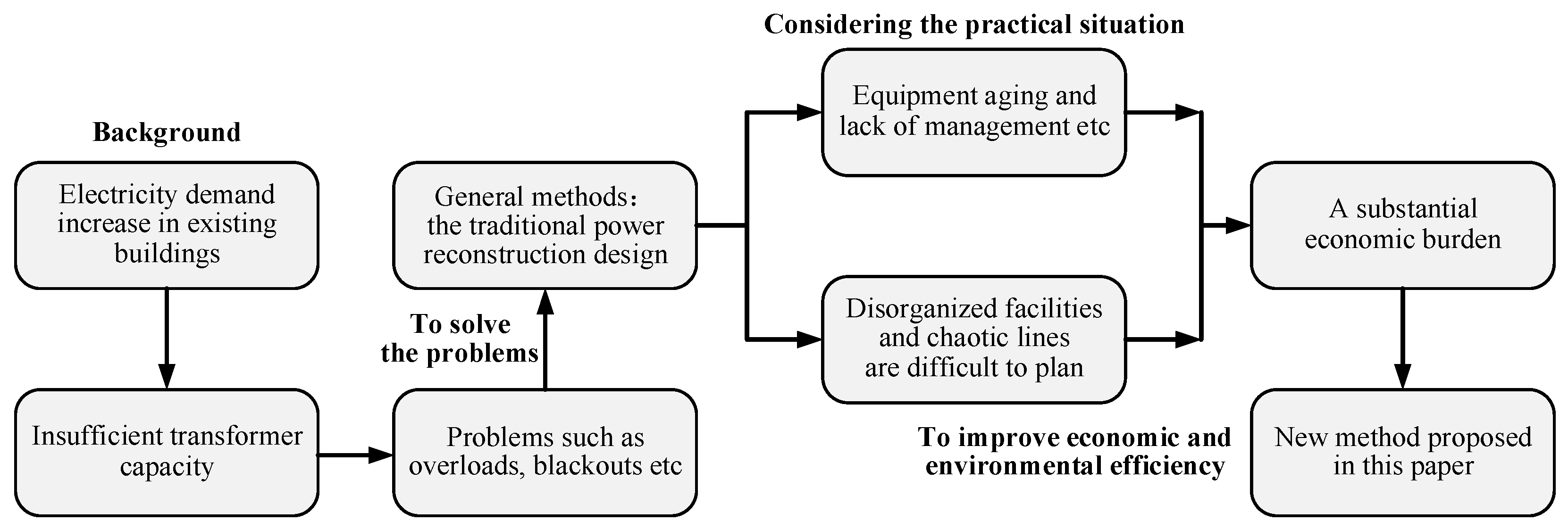
In general, the expansion of transmission capacity between buildings and the utility grid becomes necessary when the distribution system experiences frequent overload [42]. However, the reconstruction of power systems, particularly in existing buildings, presents significant challenges. The early construction of these buildings has resulted in disorganized facilities and chaotic lines, making planning difficult. Moreover, the reconstruction of an upper-level transformer substation requires the construction of power corridors. Consequently, all of these factors contribute to a substantial economic burden, as shown in Figure 1.
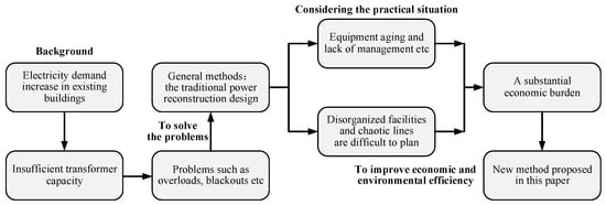
Figure 1.
The background of the new method.
Therefore, for existing buildings that face challenges in power capacity expansion and have poor economic benefits, it is feasible to retain their original power systems (including transformer configurations) and reduce their reliance on the public grid by implementing a hybrid AC/DC PV-battery (PVB) system. This can be achieved by effectively controlling the energy flow within the system, thereby ensuring that the electric power drawn from the utility grid stays within the transformer’s rated power range. The configuration method of the PVB system, including PV capacity allocation and energy storage capacity allocation, is precisely the focus of this study.
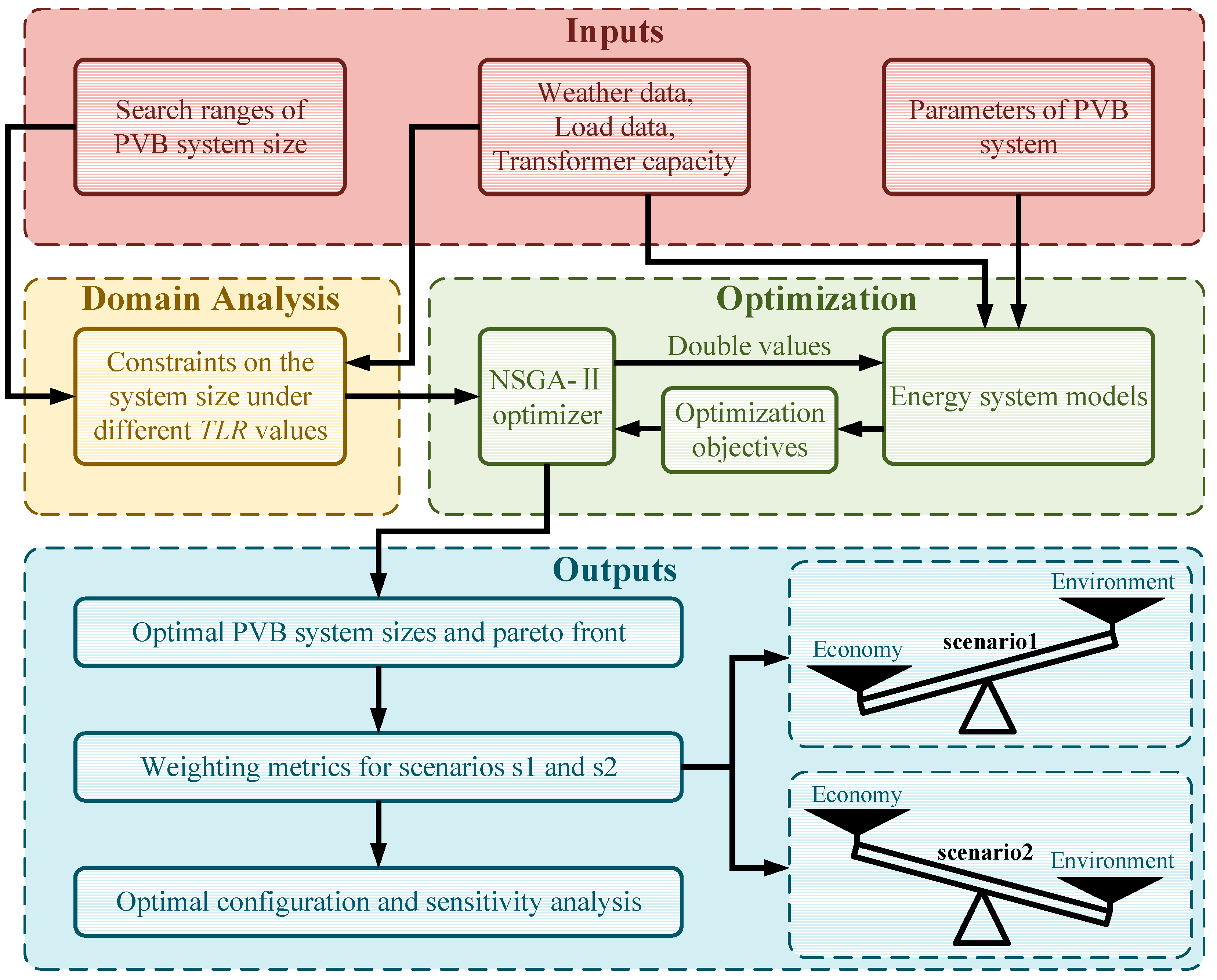
The flowchart of the optimization procedure is illustrated in Figure 2. A residential building in Shanghai and local meteorological data were selected as the simulation object. As the problem of insufficient capacity mainly occurs during the peak usage time in summer due to heightened cooling demands that drive the annual extreme transformer loading, 24 h of a typical summer day was taken as the research object. This approach captures the most severe grid stress scenario, ensuring safe operation throughout the year by addressing the extreme day balance while aligning with the optimization methodology’s focus on critical infrastructure constraints.
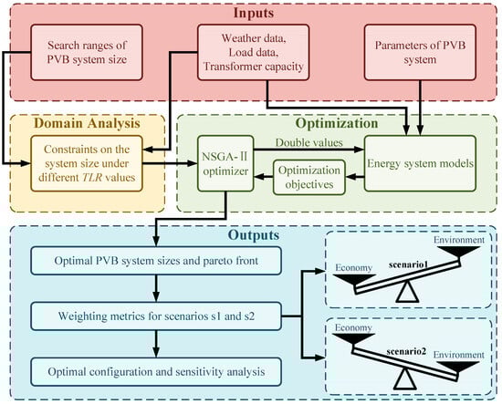
Figure 2.
Flowchart of the optimization procedure.
PVB system size ranges (PV, battery size) and other parameters serve as input for the models, along with weather data, load data, transformer capacity, and system constraints obtained through domain analysis. The NSGA-II optimization algorithm optimizes the configuration of the energy system with the objective of minimizing the two optimization objectives under the aforementioned constraints. NSGA-II is applied to determine the Pareto front sets. Then, two objective functions are weighted for two scenarios that emphasize the economy and environment, respectively. Finally, the optimal system configuration is obtained for the corresponding scenarios, and a sensitivity analysis is conducted on the configuration variables.
Consequently, based on the aforementioned technical approach, this study focuses on the following issues:
- The potential for buildings to largely maintain the current power system, while considering distributed generation on the demand side to offset the impact of loads on transmission capacity.
- Minimum required battery energy storage capacity for different PV penetration under transformer capacity constraints.
- Proposal of a multi-objective optimized approach to PVB system, based on building load power and transmission capacity, with economic and environmental performance as evaluation criteria.
- Discussion of the effects of configuration variable modifications on system performance, serving as a reference for practical engineering applications.
The paper organization is as follows. Section 2 details the system layout and optimization objectives and elaborates on the simulation models and operational strategy. In Section 3, the constraints on the system configuration range under an insufficient transformer capacity are discussed through simulations. The Pareto front solution set is obtained under the constraint by NSGA-II, and the weights of the objective functions are allocated based on the requirements of the two scenarios to calculate the optimal configuration. In Section 4, the mechanism by which the variables impact the system under the optimization method is examined. Finally, Section 5 provides the relevant conclusions.
2. Methodology
2.1. System Framework
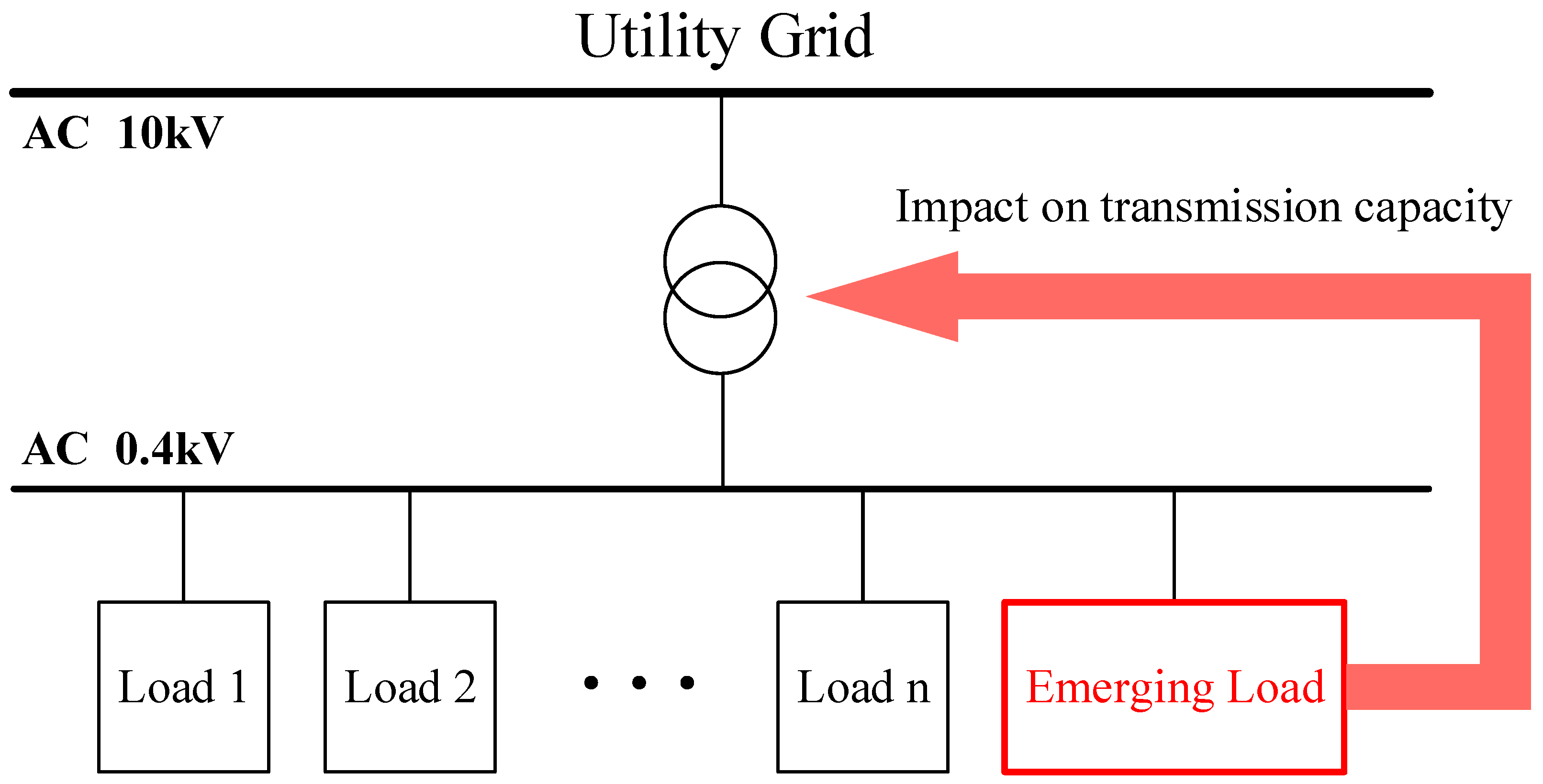
Figure 3 presents a schematic of the conventional AC distribution system found in existing buildings, which delivers electricity to users through a transformer and AC bus. Therefore, the transmission capacity is constrained by the performance of the transformer and AC bus, and can be influenced by emerging loads.
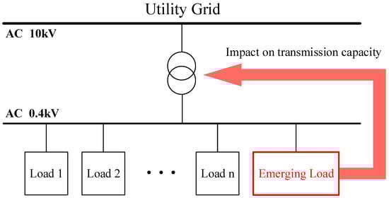
Figure 3.
Topology of the conventional AC distribution system.
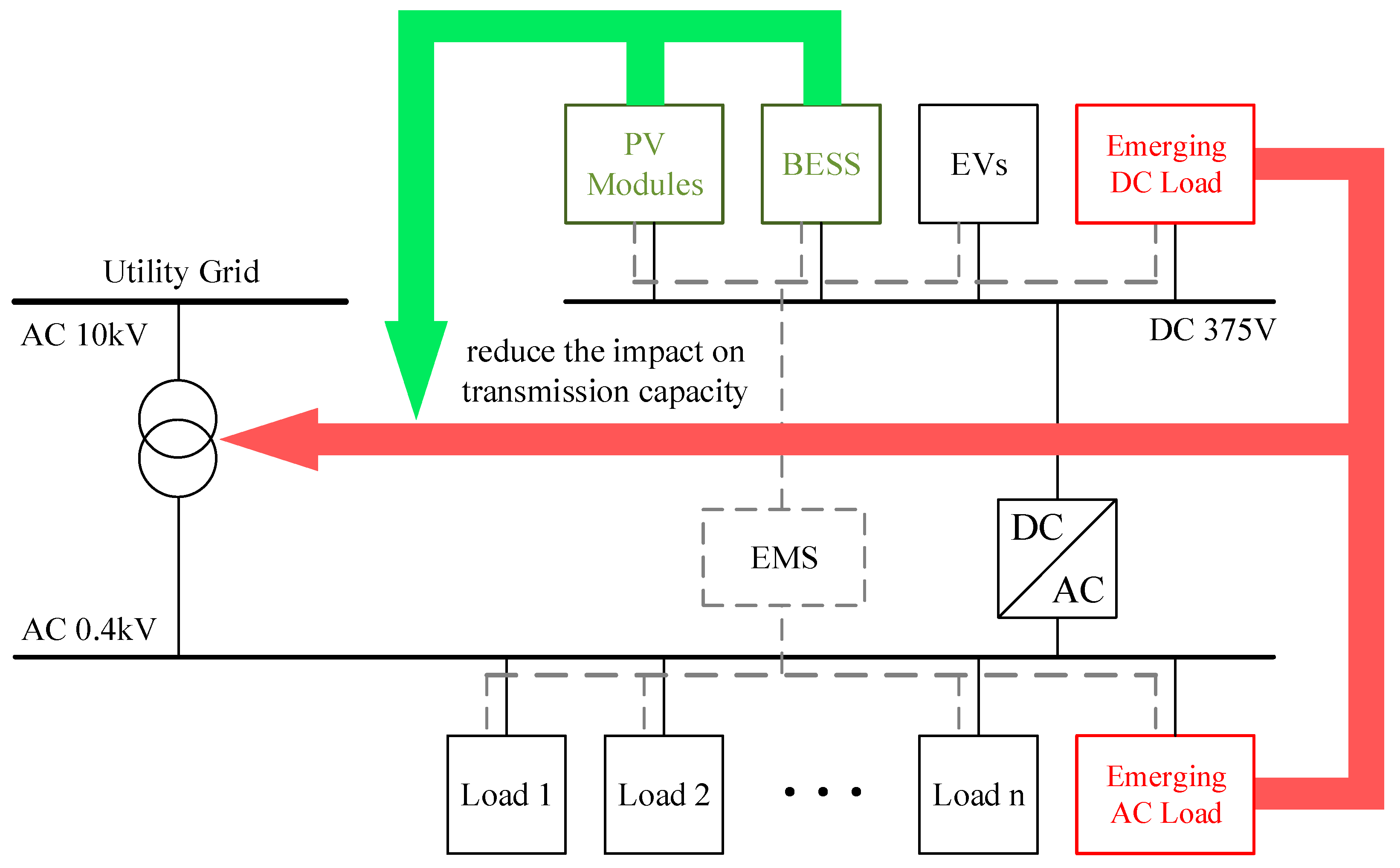
Advancements in technology have led to a surge in the adoption of DC devices, posing challenges for AC distribution systems. Frequent conversion between AC and DC reduces the energy efficiency of the distribution system. To address this issue, Figure 4 shows the proposed AC/DC hybrid PVB system for buildings. The bidirectional AC/DC converter enables simultaneous operation of the AC and DC buses. In contrast to the conventional AC distribution system, the AC/DC hybrid PVB system incorporates the concept of zoning and sub-modules to effectively differentiate between the AC and DC components, while utilizing renewable energy resources.
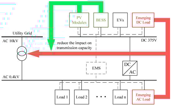
Figure 4.
Topology of the AC/DC hybrid PVB system.
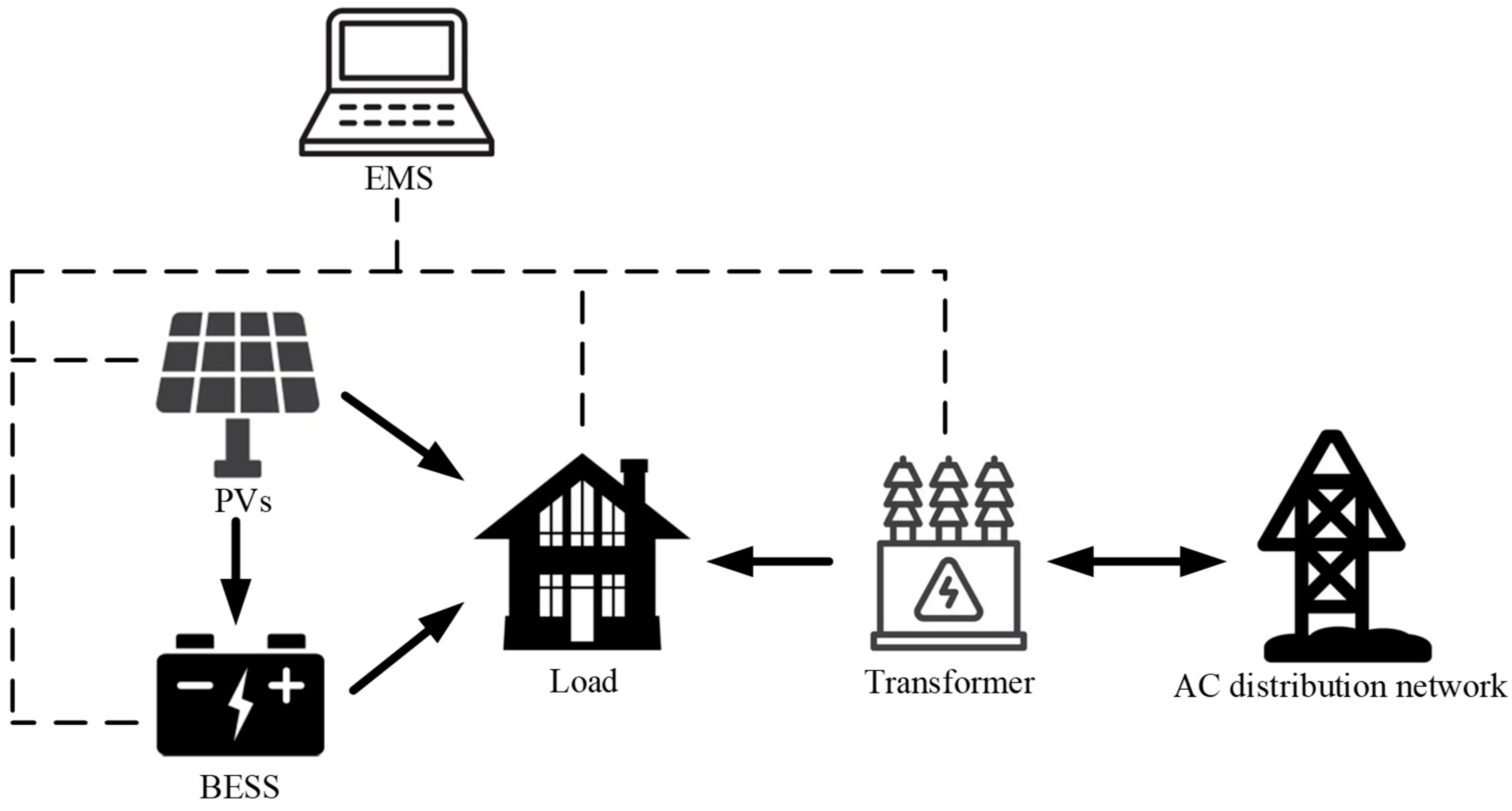
The energy generated by the PV modules is supplied to both the building load and the battery, where surplus PV power is curtailed. During PV power shortages, the battery is discharged and additional energy is imported from the utility grid to ensure continuous power delivery to the PVB system. Combined PV and BESS operation enables a reduction in the load rate on the transformer and mitigates the impact on the transmission capacity. Additionally, an energy management system (EMS) is implemented using the Internet of Things (IoT) technology, featuring a multi-load data architecture and a multi-node distributed access system (refer to Figure 5). The EMS can monitor devices and their energy data in real time, facilitating optimal control of the entire PVB system.

Figure 5.
The energy flow in the PVB system.
2.2. Optimization Objectives
This research utilizes the Diurnal Total Cost (DTC) as the model’s economic optimization criterion to gauge the financial feasibility of system investment and operational expenditures [43,44]. DTC comprises four components, (1) diurnal investment expenditure (DIN), (2) operation cost (OPE), (3) variable maintenance cost (VM), (4) fixed maintenance cost (FM), as shown in Equation (1). Equation (2) to Equation (5) enable the calculation of parts (1)–(4). Furthermore, varying operational scenarios allow for adjustments to the system configuration in each design solution. Consequently, subscript k is utilized to distinguish indicators, such as DTC, DIN, OPE, in calculations, reflecting variations across different operational scenarios. Parameters for different equipment in the system, such as C and φ, are differentiated using the subscript i.
In these equations, and represent the economic and environmental operation scenarios, respectively. CRF, the capital recovery factor, is utilized to determine the present value of an annuity (a consistent stream of equal yearly cash flows). The annual real interest rate (8%) is denoted by m, while n signifies the system’s lifespan in years. Equipment i’s capacity is represented as . The unit price of equipment i is denoted by , and its variable and fixed maintenance cost coefficients are, respectively, given by and . The quantity of electricity procured from the grid at time t is , and the corresponding purchase price per unit is .
The environmental optimization objective of the model is represented by the diurnal carbon emission (DCE) of the system [45]. The investigated system’s carbon emissions mainly originate from grid electricity purchases. In this study, the emission factor method [46] is used to calculate the DCE, as shown in Equation (7). Similarly, the DCE index also uses the subscript k to distinguish the different operation scenarios.
Diurnal carbon emission (DCE) serves as the model’s environmental optimization objective [45]. For the system under investigation, grid-purchased electricity constitutes the primary source of carbon emissions. Calculation of the DCE follows the emission factor method [46], detailed in Equation (7). Additionally, the DCE index incorporates the subscript k to differentiate among various operational scenarios. The term denotes grid emission factor.
Using the NSGA-II algorithm, the two designated objectives are optimized to generate the Pareto fronts. Therefore, a composite optimization objective function F can be defined by weighting the system’s optimization objectives, applicable to various operating scenarios, as indicated in Equation (8).
In Equation (8), the symbols and denote the decision weights assigned to the economic and environmental objectives, respectively. The terms and correspond to the minimum achievable values (or ideal targets) for economic and environmental objectives. Conversely, and represent their maximum possible values, which signify the worst-case scenario expectations for each objective. Correspondingly, and denote the and after normalization, respectively.
2.3. System Model
2.3.1. PV Generator Model
PV modules have nonlinear characteristics, and their output power is significantly dependent on solar radiation and ambient temperature. For a specific location, the power generation of a PV system is modeled through the following calculation [47,48]:
The actual power output of the PV modules, denoted by , is calculated using several parameters: (PV generator efficiency), (PV panel area in m2), and (solar radiation incident on the tilted plane in W/m2). The modules are tilted at an angle equal to the site latitude. Additional factors include (reference module efficiency), (power conditioning efficiency, set to 1 when Maximum Power Point Tracking (MPPT) is used [49]), and (the temperature coefficient for generator efficiency). Temperatures involved are (reference cell temperature in °C) and (cell temperature in °C), the latter being estimable from ambient temperature (°C) and solar radiation . The nominal operating cell temperature (NOCT) is a standard value of 45 °C [50]. Crucially, parameters , , , and NOCT vary depending on the specific PV module type and are usually supplied by the module manufacturers.
2.3.2. Battery Energy Storage System Model
During any hour, the excess power generated by the PV generators can be utilized for battery charging, while the stored energy can be discharged when power generation falls short. Therefore, the difference between the energy generated and the load demand determines whether the battery is in a charging or discharging state. The state of charge (SOC) is commonly used to describe the charging and discharging state of batteries, and is defined as the ratio of the energy content of the battery () to its rated capacity () in Equation (10).
Within each hour, surplus energy from the PV units can charge the batteries. Conversely, stored energy is discharged when generation cannot meet demand. Consequently, the net energy balance (generation minus load demand) dictates the battery’s operating mode: charging or discharging. The battery’s state of charge (SOC), a standard indicator for its energy level, is expressed as the proportion of its current stored energy () to its rated capacity (), as defined in Equation (10).
The battery’s functioning status comprises two primary phases: charging and discharging. During the operation of the battery, SOC can be expressed as follows [51]:
where indicates the actual operating power of the battery, and correspond to the charging power ( > 0) and discharging power of the battery ( < 0), respectively. In addition, is a binary number, where 1 represents the battery charging state and 0 represents the battery discharging state. and denote the efficacy rates for battery charging and discharging, respectively. signifies the discrete temporal interval for simulation, which is taken as 1 s in this study.
At any time t, the charged quantity and the operating power of the battery are governed by the following constraints:
where signifies the battery’s maximum charge capacity, while _min denotes its minimum charge capacity; and and are the maximum charging power and maximum charging power, respectively.
2.4. System Operation Strategy
To gain complete insight into operation strategy, it is imperative to establish the parameters for different simulation scenarios. PV penetration () is typically expressed as the quotient between the total photovoltaic generation () and the building load () [52]. To quantify the transmission capacity between buildings and the utility grid, this study defines the transmission limit ratio () as the ratio between the maximum transmission power () and the building load’s peak power (). and are important dimensionless variables in this study, and their expressions are shown in Equation (13).
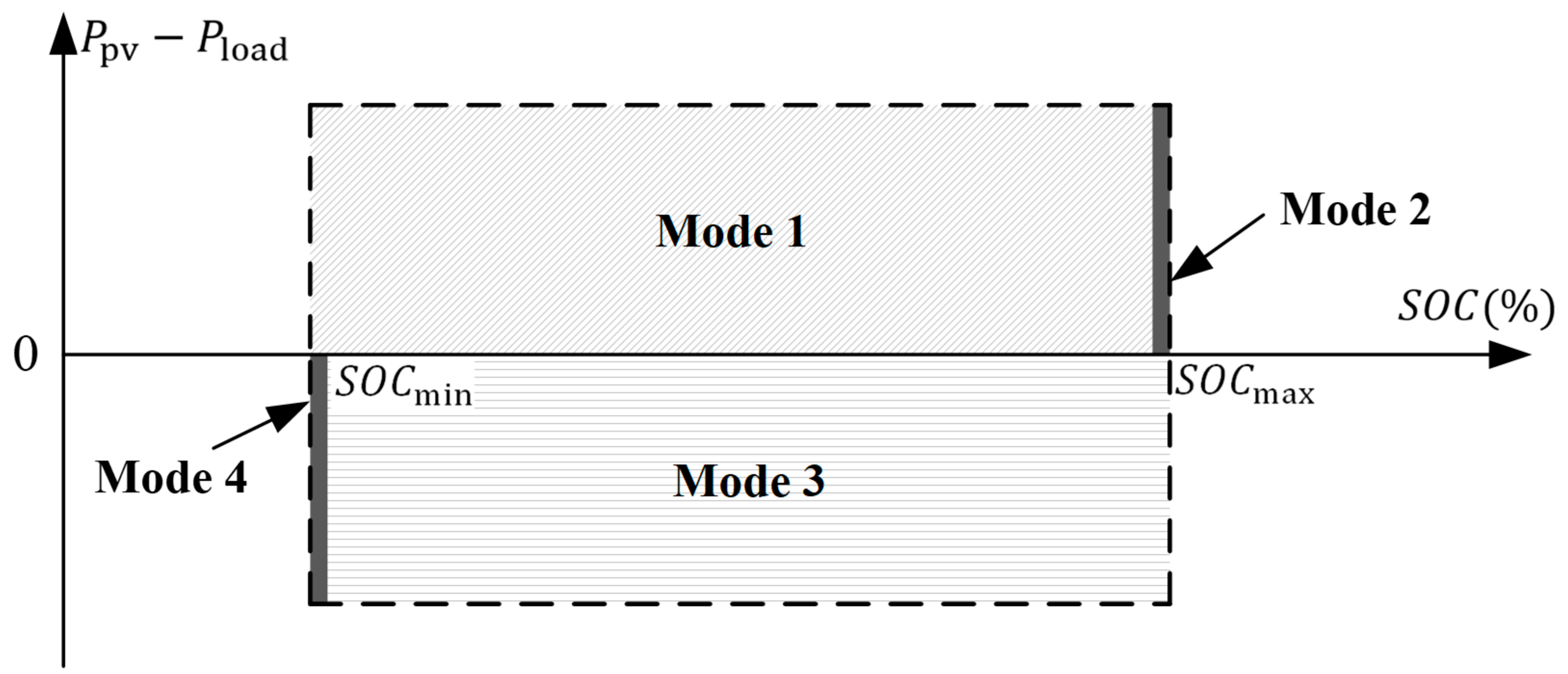
This study aims to configure the BESS optimally and reduce DTC and DCE, subject to the constraints imposed by the existing building’s transmission capacity. The charging or discharging state of the battery is governed by the disparity between generated PV energy and load energy demand. Therefore, based on the difference between and , the operational state of the system can be classified into four modes, as illustrated in Figure 6.
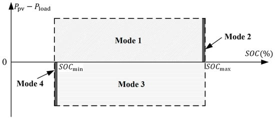
Figure 6.
Operation mode division diagram.
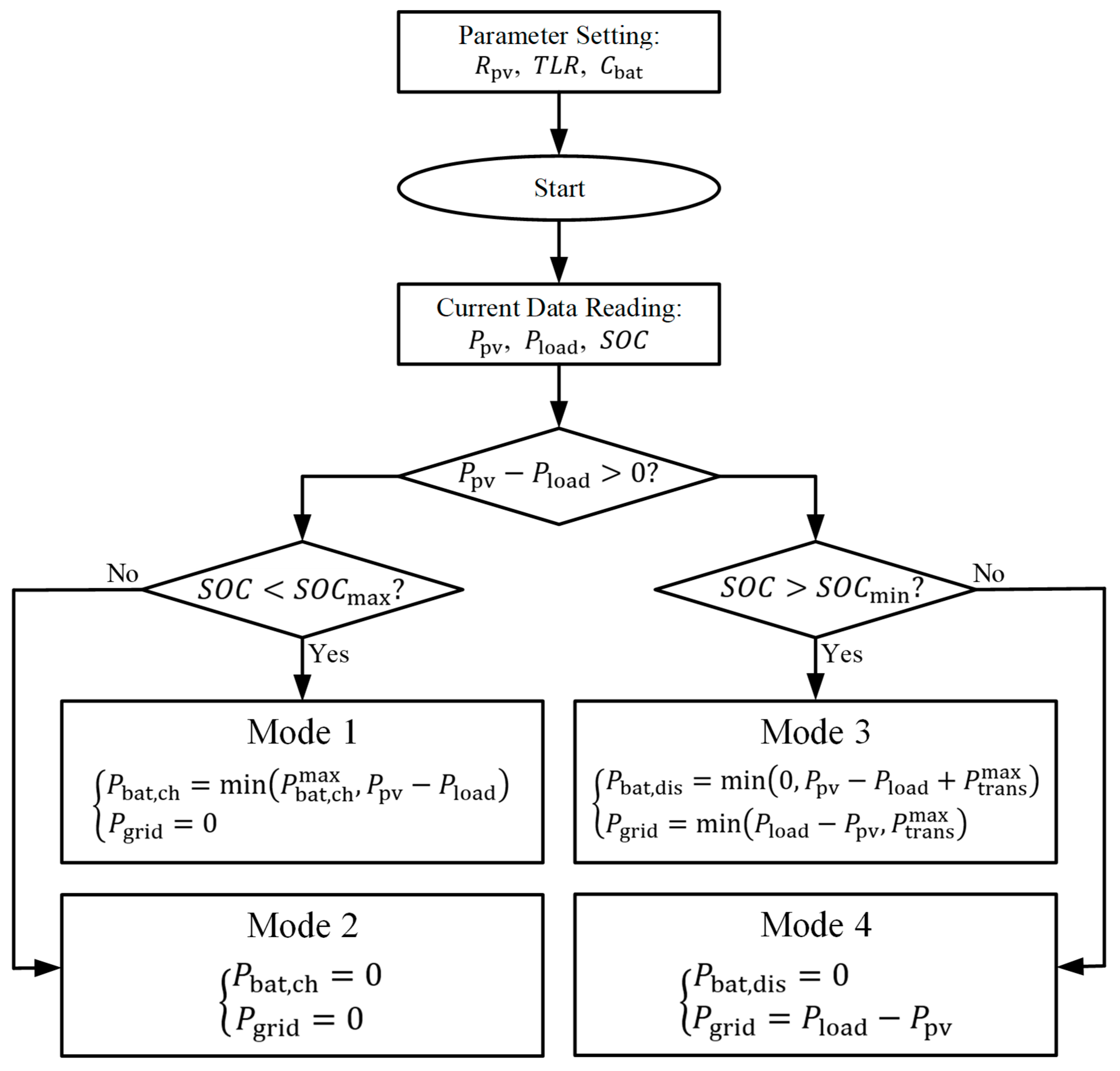
Based on the classification of modes, an appropriate operation strategy was formulated to effectively manage the energy flow within the PVB system. Figure 7 depicts the system’s operational strategy. The battery stores energy during intervals of excess PV generation and discharges power when PV output is inadequate to satisfy the building’s demand. Crucially, if exceeds , the PVB system gives precedence to procuring electricity from the power grid. Should the net load (defined as minus ) surpass , the battery supplies the additional power requirement. From an energy balance perspective, the power constraint is given by the following equation:
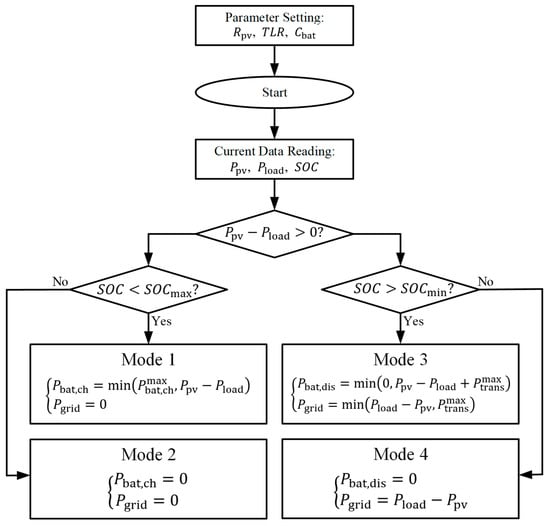
Figure 7.
Flow chart of the system operation strategy.
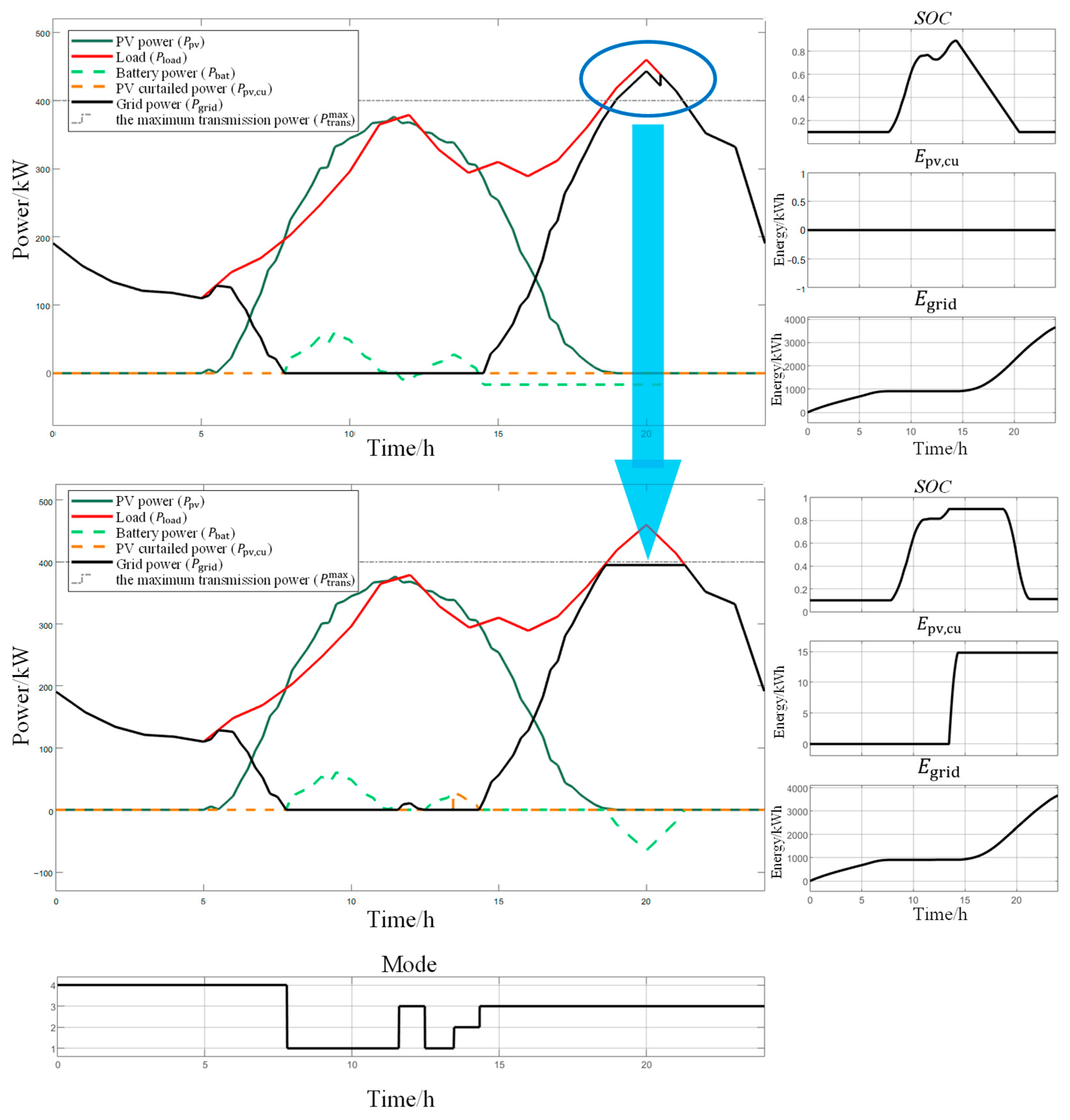
To clearly express the control effect, the net load () is introduced (as shown in Equation (15)), which is defined as the difference between and . The three power curves are plotted in Figure 8. To further illustrate the relationship between the energy flows, the available surplus PV output and the net load exceeding the maximum transmission power are represented by and , respectively (as shown in the green and red areas). Obviously, the blue and green areas have the same area, both representing . The main objective of the control strategy is to store through BESS to supply power to , while ensuring that the power supply from the grid does not exceed , as depicted in Figure 9. and can also be calculated using the following formulas.
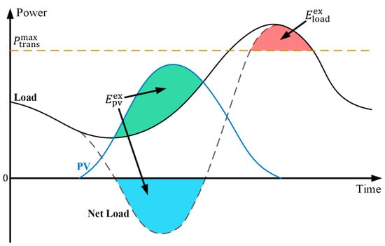
Figure 8.
Schematic diagram of control effect.
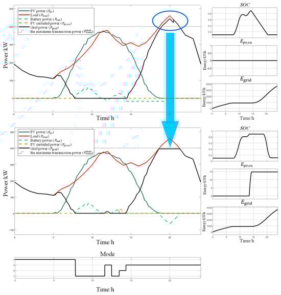
Figure 9.
Schematic diagram of simulated diurnal operation.
3. Case Study and Results
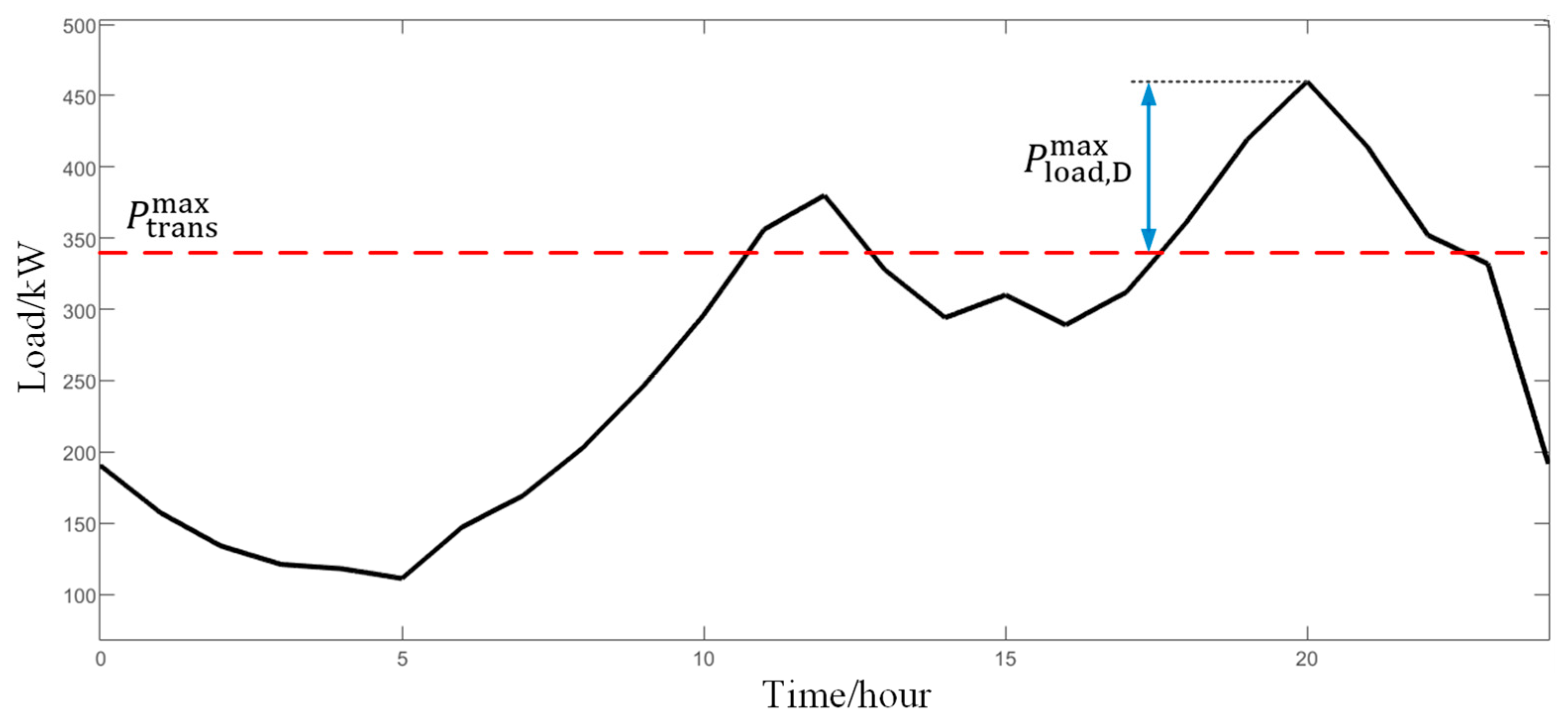
First, the typical daily load of a residential building in Shanghai is selected as the research object of this study, with a summer day chosen due to its load profile, dominated by peak cooling consumption, exhibiting the annual maximum transformer stress. This makes it a conservative benchmark for capacity constraints under extreme conditions. As shown in Figure 10, for ease of description, the peak load value above is defined as , which can be determined as follows:
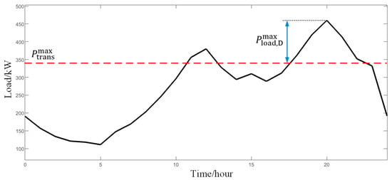
Figure 10.
The typical diurnal load curve.
Because this study mainly focuses on the situation where is less than , must be greater than 0, and similarly, TLR must be less than 1. According to the definition of , the maximum net load curve exceeding is calculated as follows:
Table 1 details the battery parameters used for this research.

Table 1.
Battery parameters.
The parameters of optimization objectives can be found in Table 2.
Table 2.
The parameter settings of the optimization objectives.
In the case study, a time-of-use electricity pricing scheme was employed for Shanghai residential electricity tariffs (), as detailed in Table 3. Electricity rates are higher during the high-demand hours (6:00 AM to 10:00 PM) at 0.0897 USD per kWh. Conversely, the lower rate of 0.0446 USD per kWh applies during off-peak periods, which run from midnight to 6:00 AM and 10:00 PM to midnight.
Table 3.
Shanghai residential time-of-use electricity pricing schedule.
3.1. Domain Analysis of the System
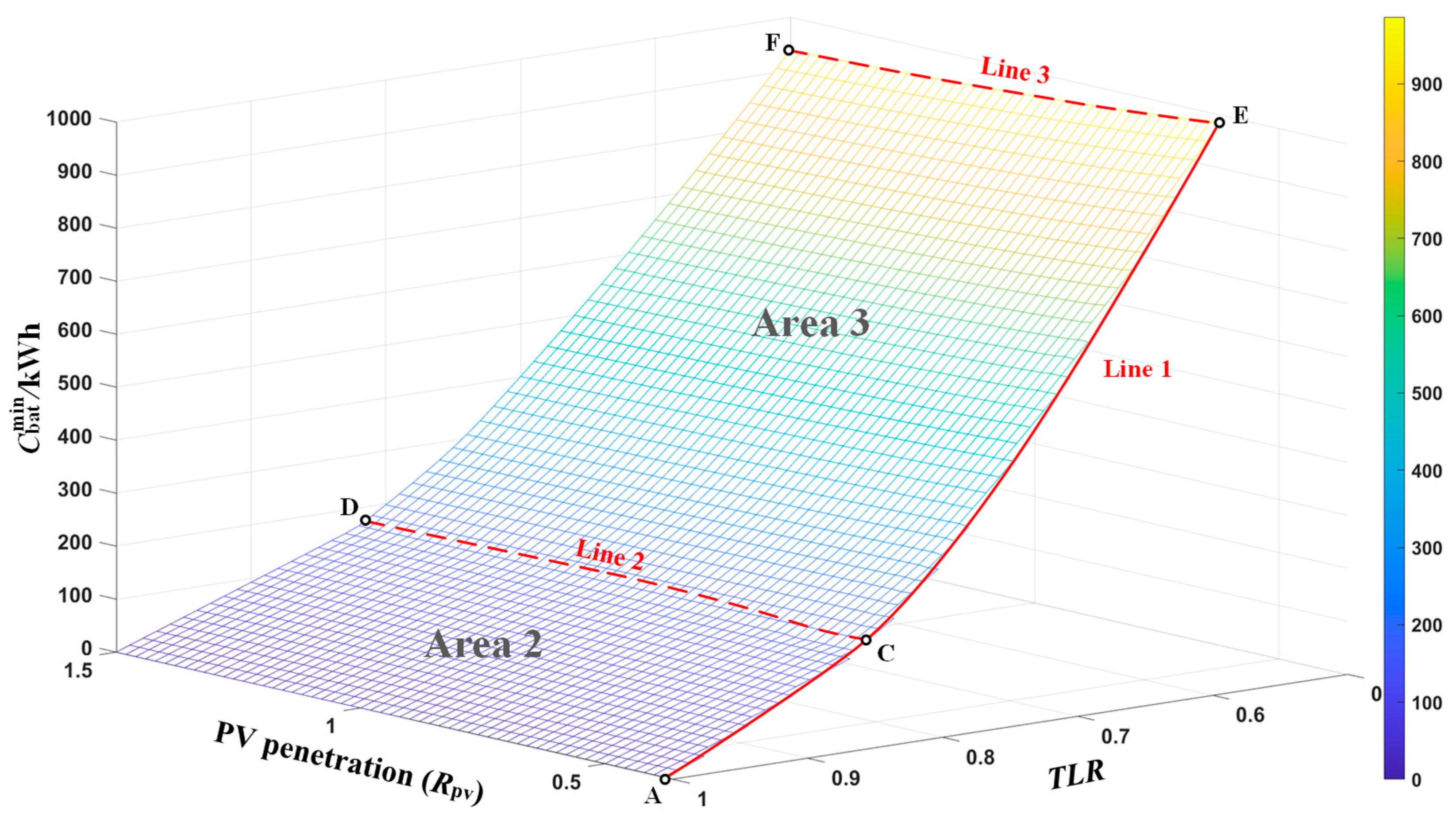
Considering the limitations of transformer capacity, there should exist a minimum storage capacity () under each TLR value and , which can meet the minimum requirements for the normal operation of the system. The , along with the corresponding and TLR values, can provide constraints for the search range in subsequent multi-objective optimizations. Therefore, before optimizing the system configuration, it is necessary to simulate the above constraints to obtain an effective region within the independent variable domain.
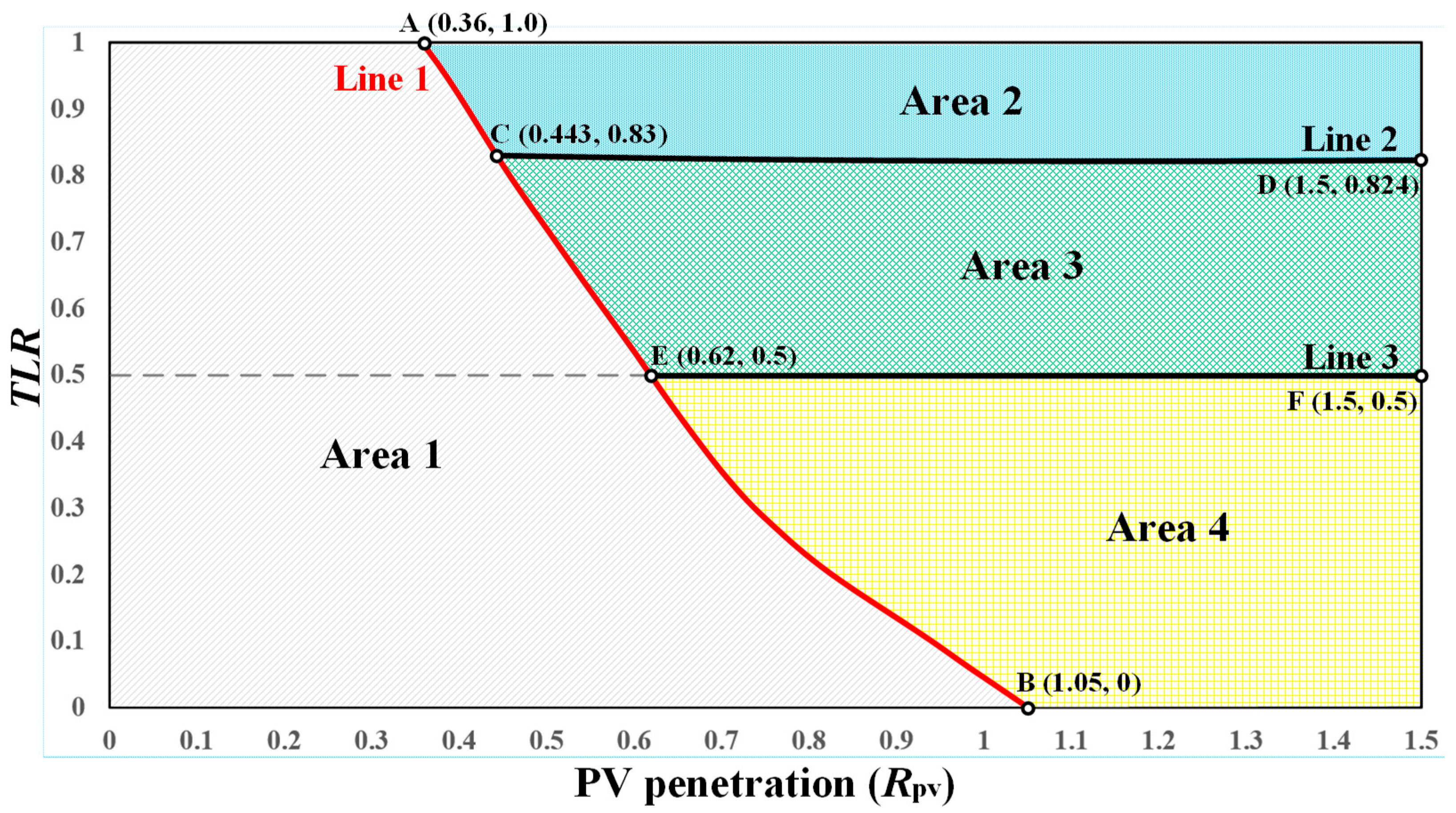
A Cartesian coordinate system is established featuring on the x-axis, with TLR assigned to the y-axis. To obtain universally applicable research results, the range of is set from 0 to 1.5, while the range of TLR values is limited to 0 to 1. Figure 11 presents the results from simulating the boundary conditions. It is obvious that not every point in the coordinate system has a corresponding . Overall, the coordinate system can be divided into four regions by using three lines.

Figure 11.
System domain diagram.
Based on the energy relationship in Figure 8, it is evident that to guarantee standard daily operation of the system, must be greater than . Considering the energy loss resulting from battery charge/discharge cycles, Line 1 can be derived through simulation, as shown by the red line in Figure 11. It is apparent that as increases, TLR gradually decreases, with the rate of decrease diminishing. This can be attributed to higher leading to greater availability of photovoltaic power generation, thereby reducing the demand for transmission capacity from the grid (i.e., TLR value). From an energy perspective, does not theoretically exist in Area 1, so this paper will not further discuss this area.
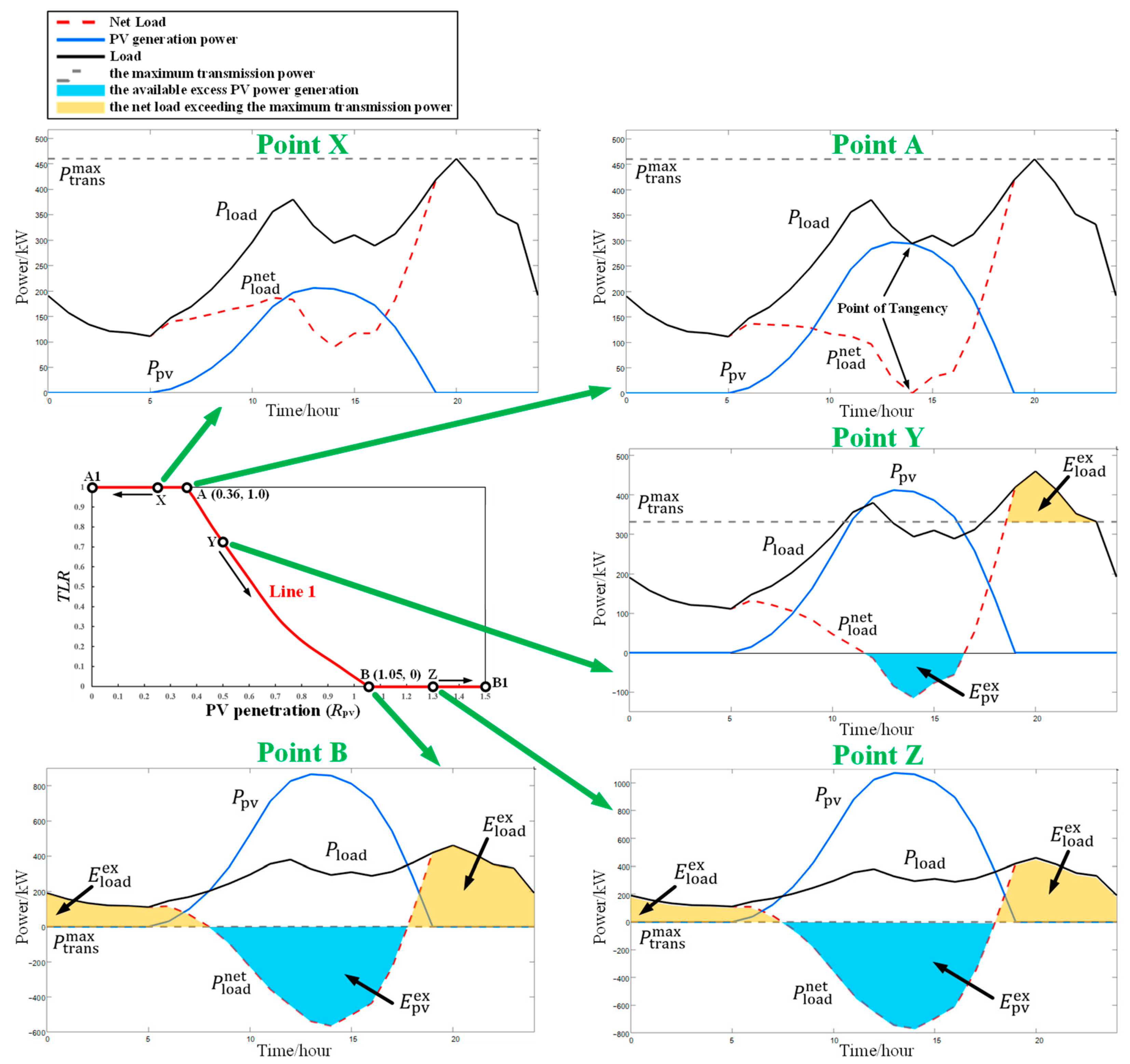
To better illustrate the physical meaning of Line 1, line segment AA1 is constructed perpendicular to the y-axis passing through point A, intersecting the y-axis at point A1. Point B extends to the right along the x-axis to point B1. The moving points X, Y, and Z are located on segments AA1, AB, and BB1, respectively (excluding the two endpoints of each segment). The system analysis corresponding to these points is shown in Figure 12.

Figure 12.
System analysis of each point on Line 1.
The at point X is extremely low, resulting in always being greater than 0. This implies that the PV output curve is consistently below the load curve, leading to the absence of in this situation. As the increases, the critical point (point A) reaches 0.36. At point A, a tangent point is formed between the PV output curve and load curve. Correspondingly, the net load curve is tangent to the X-axis, where is equal to zero. Along line AB, both and increase simultaneously with the increase in . However, remains equal to after energy loss. As continues to increase, a new critical point (point B) is reached. At point B, the TLR has dropped to 0, while after energy loss remains equal to . This indicates that the system no longer requires electricity from the grid and can utilize effective energy flow planning to fulfill the complete daily energy requirements solely with PV generation, thereby achieving a fully self-sufficient power supply mode. On segment BB1, as further increases, decreases while increases, as shown at point Z. Excess PV power generation can be curtailed or transmitted to the utility grid. A summary of the system analysis corresponding to the relevant points in Line 1 is shown in Table 4.
Table 4.
System analysis corresponding to each point.
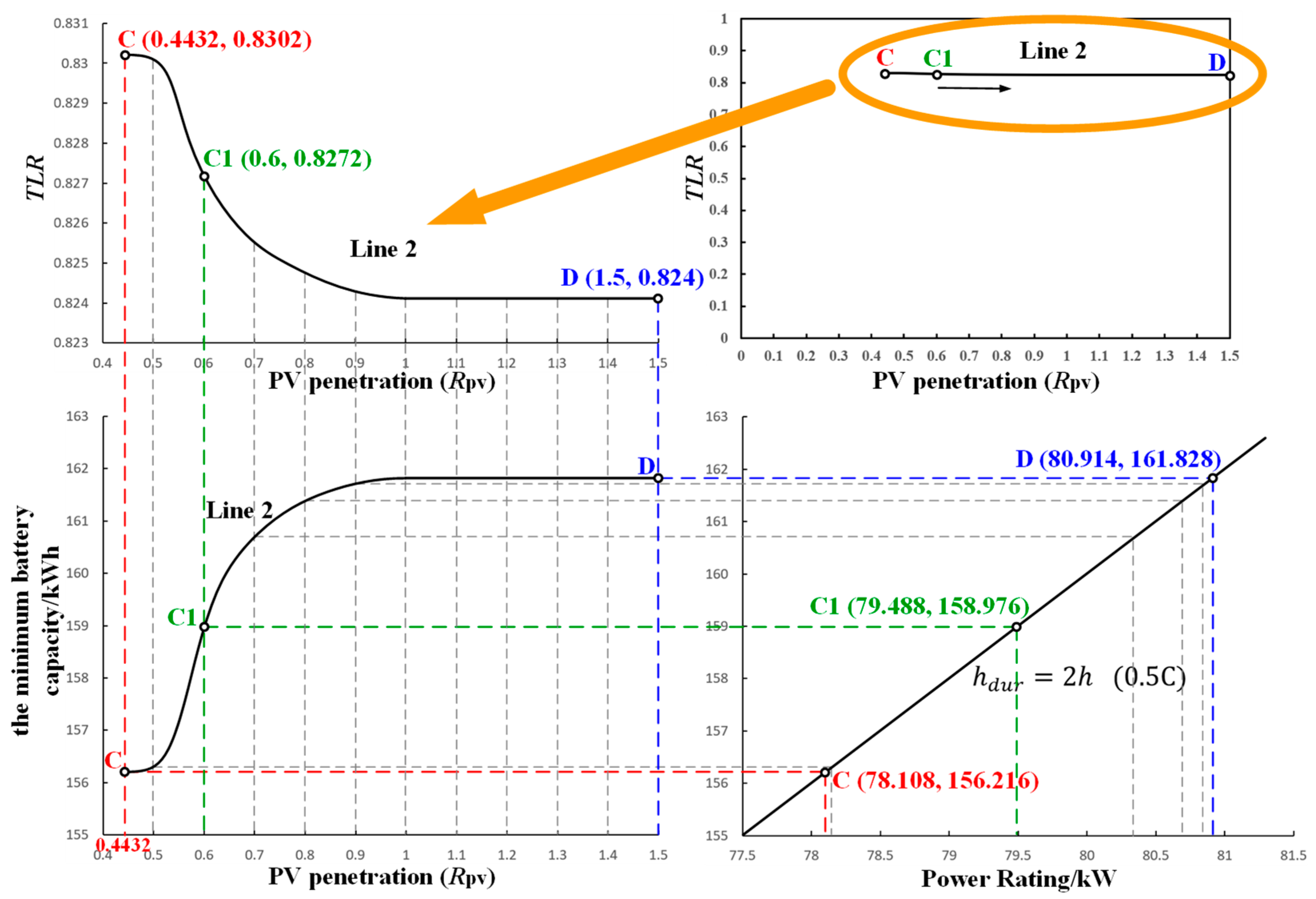
Under the premise of the energy relationship (on the right side of Line 1), the configuration of the energy storage capacity () cannot be based solely on . Due to the high-power demands of peak loads on the battery, the necessary capacity may exceed the minimum value theoretically required based on energy needs alone, when accounting for charge–discharge rate limitations. To determine the critical point of this relationship, Line 2 is derived through simulation, as shown in Figure 11. However, Line 2 appears as an approximately straight line in Figure 11 and lacks clear features. Therefore, it is magnified and presented in Figure 13.
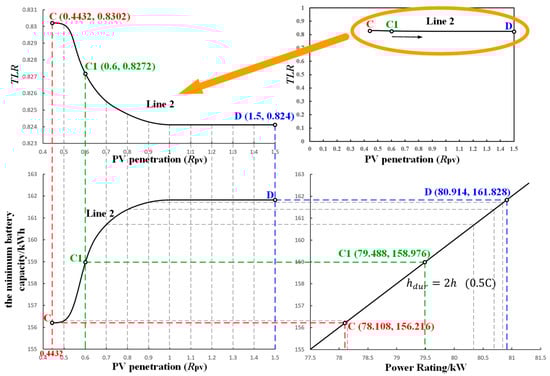
Figure 13.
Line 2 and corresponding energy storage capacity.
The characteristic curves demonstrate that as increases, TLR gradually decreases and eventually stabilizes at 0.824. Similarly, as increases, gradually increases and then stabilizes at 161.828 kWh. This is because a higher implies a lower under the same TLR condition. Therefore, TLR can be further reduced to achieve a larger until under each exhibits the same multiple relationship with , resulting in a higher required . Furthermore, in the lower right portion of Figure 13, the and maximum battery discharge power required for each point on Line 2 are located on the previously defined battery characteristic line, with a maximum charging/discharging rate of 0.5 C.
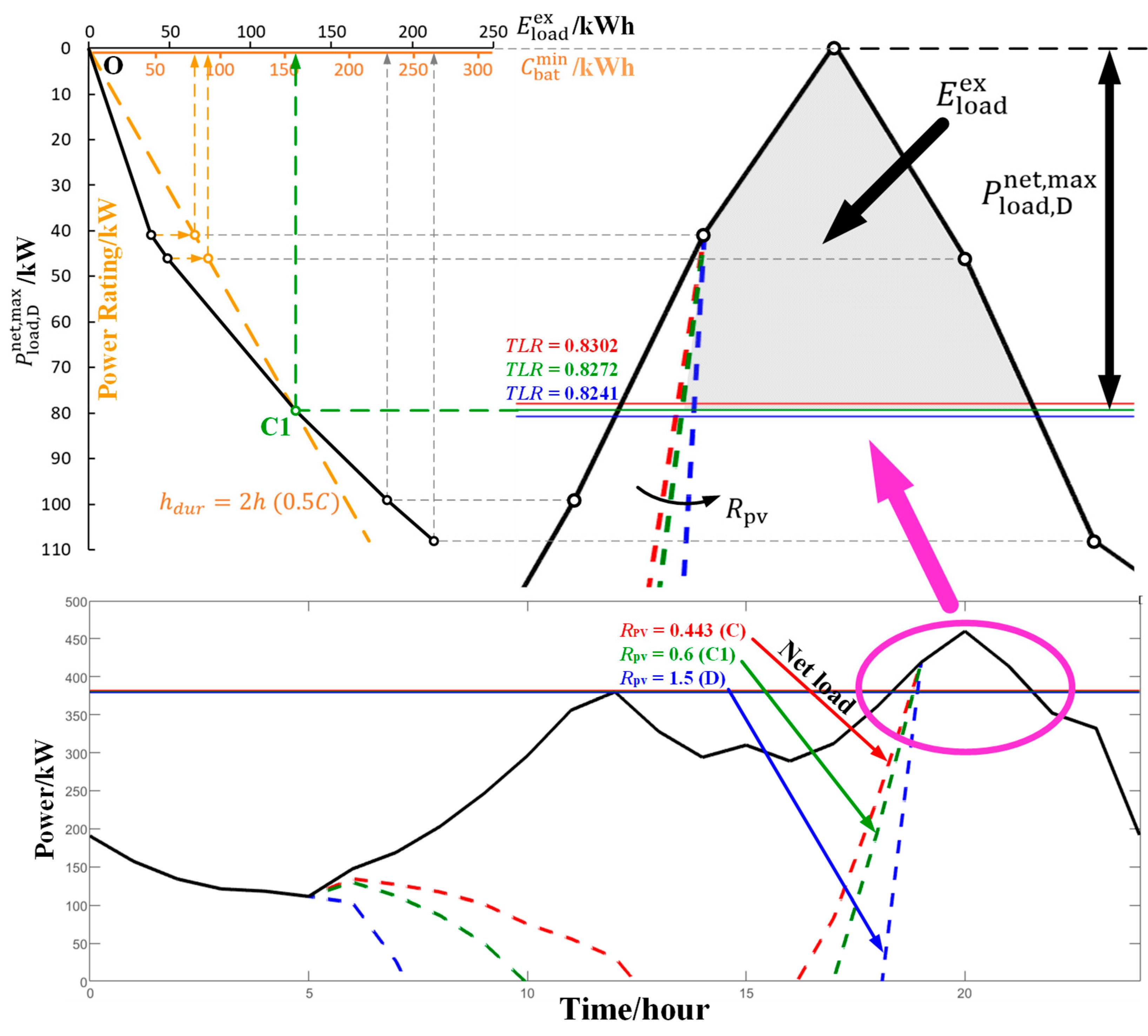
To further analyze the situation at each point on Line 2, point C1 (with a of 0.6) is selected, and a line chart illustrating the corresponding (black axis) and (orange axis) values for its TLR (0.8272) is presented in Figure 14. is selected as the y-axis in the figure to facilitate the description of the energy and power relationship.
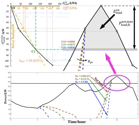
Figure 14.
Energy and power curve at point C1.
In Figure 14, the corresponding to is represented by the black solid line, while the battery characteristics are depicted by the orange dashed line. Along the OC1 line, the is determined by the energy storage capacity corresponding to the battery characteristics at the same value, as indicated by the orange arrow. Beyond point C1, the corresponding can be directly determined based on the curve, as shown by the grey arrow. Point C1 serves as a critical point on the line where the is 0.6. Furthermore, Line 2 is formed by connecting the critical points at different values. In Area 2 above Line 2, the value of is selected based on the battery characteristics (orange dashed line). In the area below Line 2, the value of is calculated based on the energy relationship (black solid line).
Line 3 in Figure 11 is a straight line with a TLR value of 0.5. Area 4 below Line 3 is characterized by a low transmission capacity of the power grid, making it more suitable for traditional power expansion methods. Therefore, this study does not delve into the discussion in Area 4. This study mainly focuses on Areas 2 and 3.
3.2. Capacity Analysis of Energy Storage System
The results of the battery capacity configuration after the simulation within the domain of and TLR are shown in Figure 15. It can be observed that is negatively correlated with the and positively correlated with the TLR value. Additionally, the growth rate of with increasing TLR is comparatively moderate in Area 2, while in Area 3, the increase in with TLR is more pronounced.
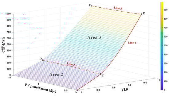
Figure 15.
distribution diagram.
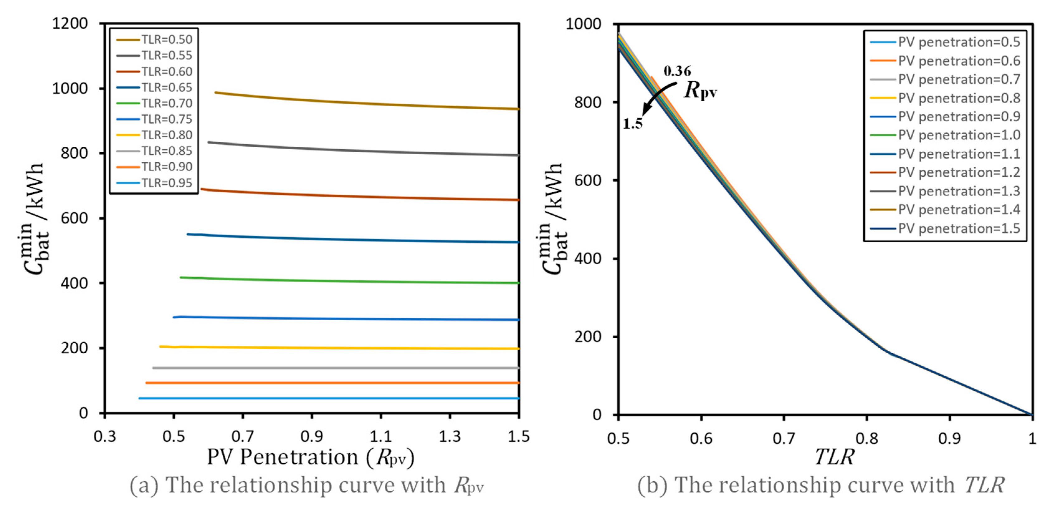
To more thoroughly examine how variables influence , the relationship curves between and , as well as TLR values, are shown in Figure 16. Analysis shows that TLR values have a significant influence on . A decreasing TLR value indicates a more severe system power capacity shortage, necessitating greater renewable energy integration and larger associated storage capacity. In contrast, the impact of on is relatively small. As the increases, the required storage capacity of the system gradually decreases.
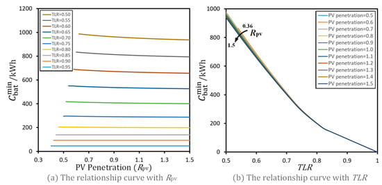
Figure 16.
The relationship curves of .
3.3. Optimization Results and Analysis
Based on domain analysis in Section 3.1 and the storage capacity analysis in Section 3.2, system configuration optimization needs to be conducted under the following constraints:
In Equation (18), A represents the effective definition domain of and TLR, that is, the union set of Areas 2 and 3 in Figure 11.
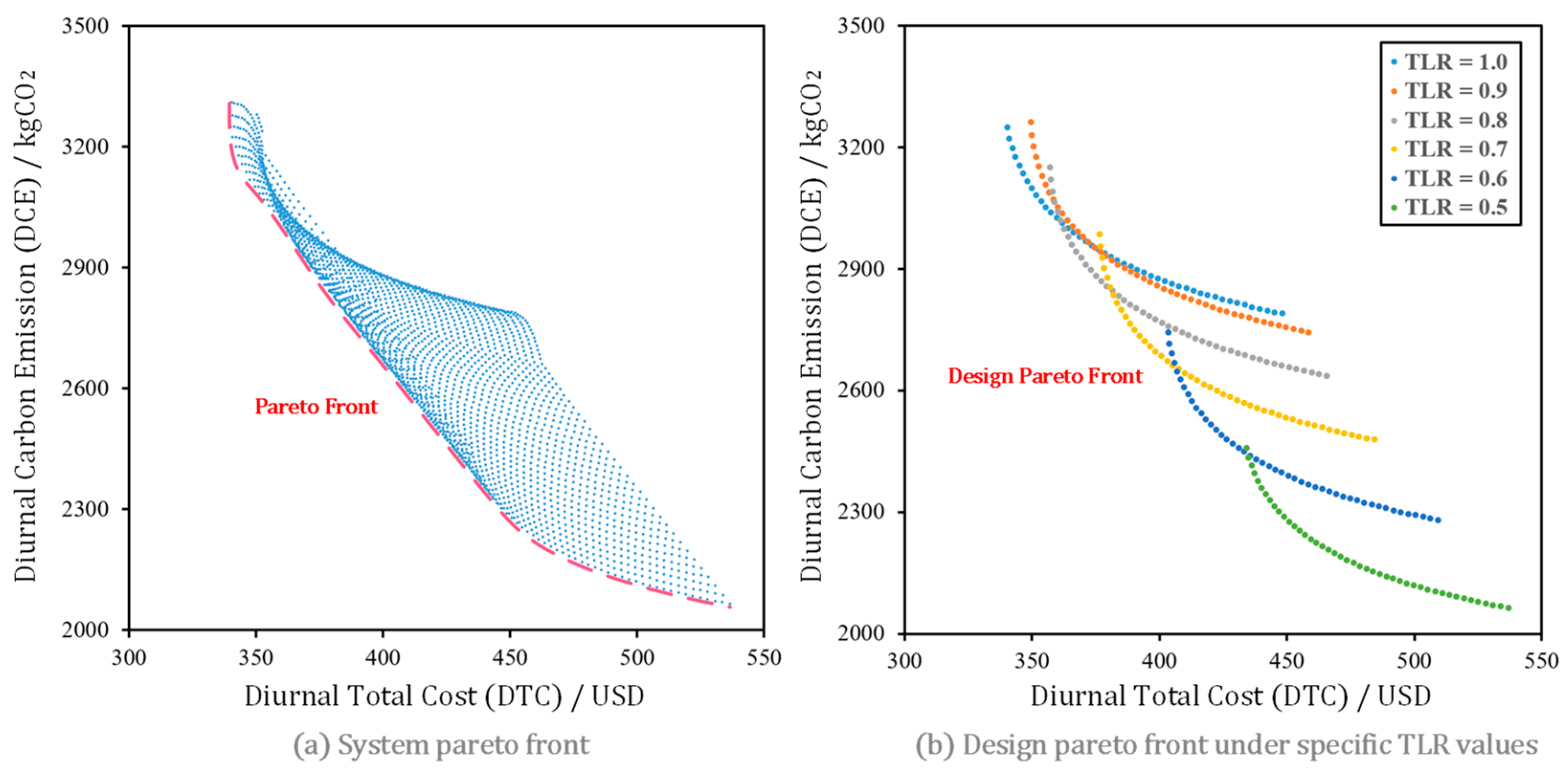
The Pareto front generated by NSGA-II is shown in Figure 17. In Figure 17a, the blue points are the designed Pareto front solution sets corresponding to the TLR values. The Pareto front of these points is represented by the red dashed line, that is, the Pareto-optimal sets of the PVB system. However, it should be taken into account that in practical engineering applications, TLR is a fixed value and not a variable that can be optimized and adjusted. Therefore, in Figure 17b, the design Pareto front sets of the system under specific TLR values are shown separately. Each curve represents the optimal solution set for the PVB system design stage under the current TLR value.
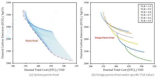
Figure 17.
The pareto-optimal sets of PVB system.
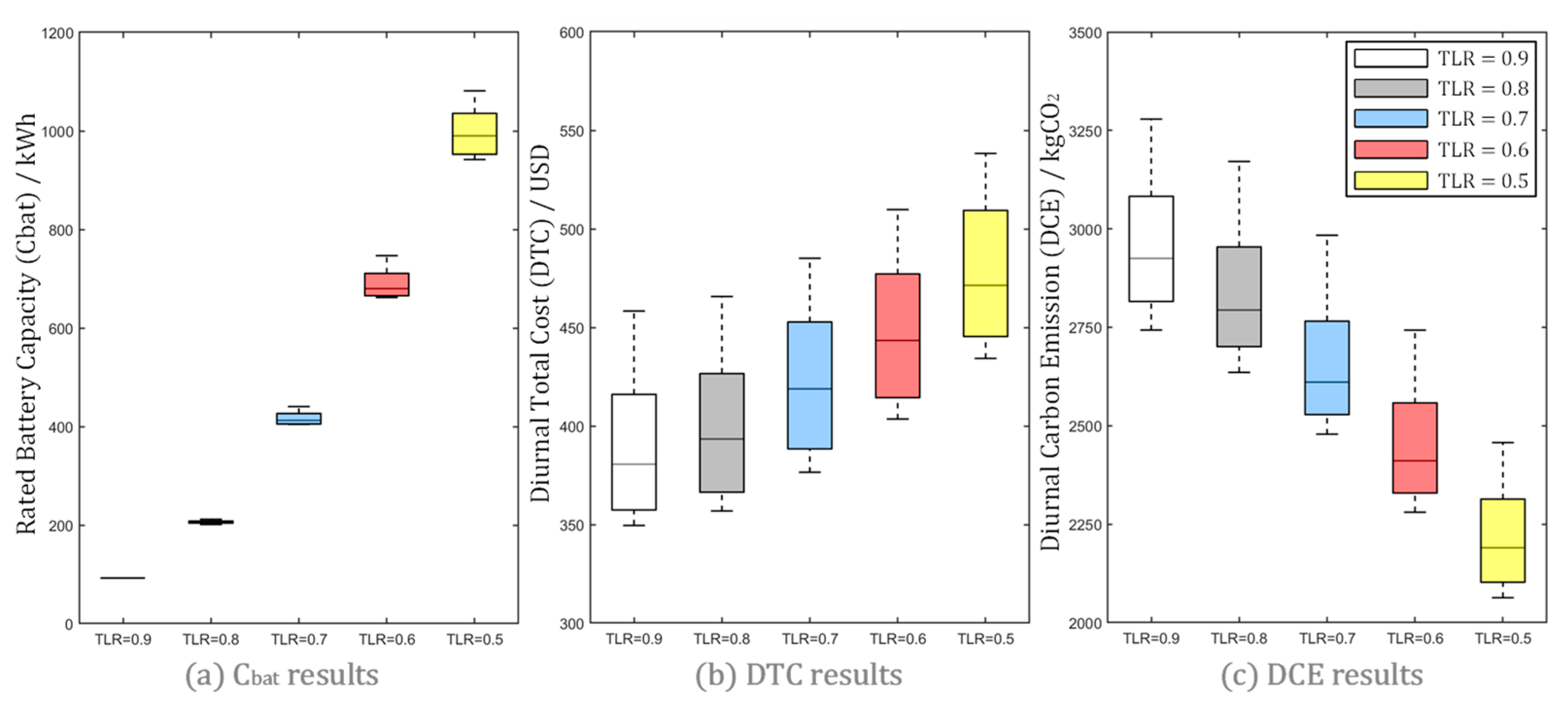
Figure 18 shows the distribution of the battery capacity configuration, DTC, and DCE across the optimized solution groups at different TLR levels. The chart shows that smaller TLR values require larger storage capacity. When TLR is 0.9, a 100kWh battery is configured, while when TLR is 0.5, a battery with a capacity of up to approximately 1000 kWh needs to be configured to meet optimization. High-capacity storage equipment incurs higher costs, which increases the DTC. Correspondingly, high-capacity storage equipment can effectively reduce DCE and is more environmentally friendly.
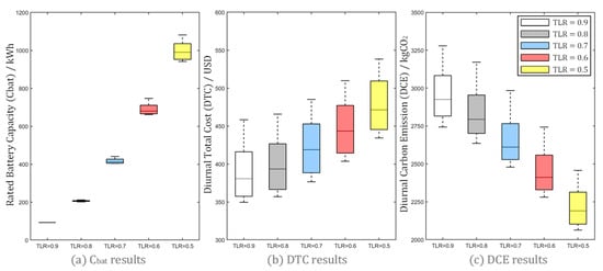
Figure 18.
Analysis of configuration and optimization objectives under different TLR values.
After obtaining the optimal solution sets for each TLR value, another step is to assign decision weights to each objective based on the two scenarios. Table 5 is a pairwise comparison matrix constructed based on the scores given by the experts for each objective. Scores range from 1 to 9, where a score of 1 indicates two equally important objectives, and a score of 9 indicates that one objective is much more important than the other [56]. To validate the acceptability of the subjective scoring matrix, the decision matrix’s consistency ratio should remain below 0.1 [57]. Given that stakeholders assign differing priorities to each objective, this research incorporates two distinct sets of decision weights for stakeholders with varying emphases, presented in Table 5.
Table 5.
Decision matrix of scenarios and .
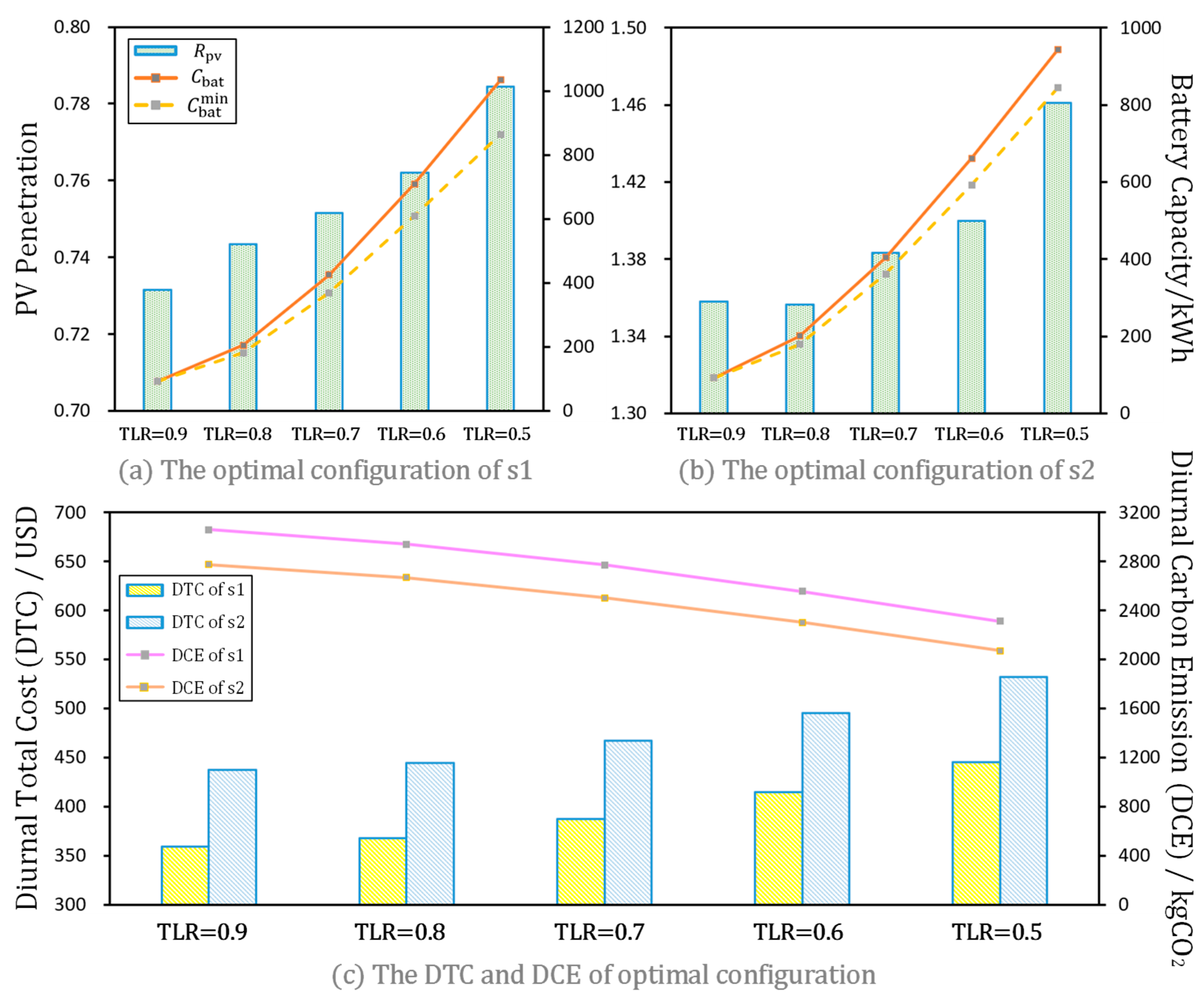
Based on the weights in Table 5, the optimal configurations corresponding to different TLR values for scenarios and can be calculated, as shown in Table 6 and Figure 19. In both scenarios, as TLR decreases, the required configuration capacities for both PV and energy storage increase. The demand for increased energy storage capacity is significantly higher than that for increased PV capacity. This is because increasing energy storage capacity to address peak loads is more economical compared to increasing PV configuration capacity. Additionally, equipment capacity expansion is necessary to accommodate the growing user load, which implies an increase in DTC. This increased economic investment yields favorable environmental benefits, namely a reduction in the value of DCE.
Table 6.
The optimal configurations for scenarios and .

Figure 19.
Analysis of the optimal configurations for scenarios and .
Comparing the two scenarios, under the same TLR value, the difference between in scenario and is large, while the difference between is small. Between different TLR values in the same scenario, the difference between is small, while the change in is large. Therefore, it can be considered that is the key factor that distinguishes between the two scenarios, while mainly distinguishes different TLR values. The size of can be adjusted to achieve the conversion between economic scenarios and environmental scenarios, while the size of is mainly used to meet the safe operation of the system under different TLR values (i.e., the is to some extent higher than the in the corresponding case).
4. Discussion
The domain analysis in Section 3.1 determines which combinations (i.e., the corresponding areas in the domain) will have feasible system configuration solutions, thus guaranteeing secure system functioning during scenarios of inadequate transformer capacity. In Section 3.2, battery storage capacity analysis calculates the minimum storage capacity() corresponding to each point within the feasible domain (i.e., Areas 2 and 3). Therefore, the conclusions of Section 3.1 and Section 3.2 provide constraint conditions for the variable values from the perspective of system safe operation for the multi-objective optimization in Section 3.3.
Section 3.3 employs the NSGA-II algorithm with two objective functions to derive the optimal system configuration solution set, presenting tailored optimal configurations for distinct scenarios. Next, this section discusses the impact mechanism of the variables (i.e., A and B under a fixed TLR) on the system in the optimization method, and explores the limitations of the current study.
4.1. Analysis of Changes in Independent Variables
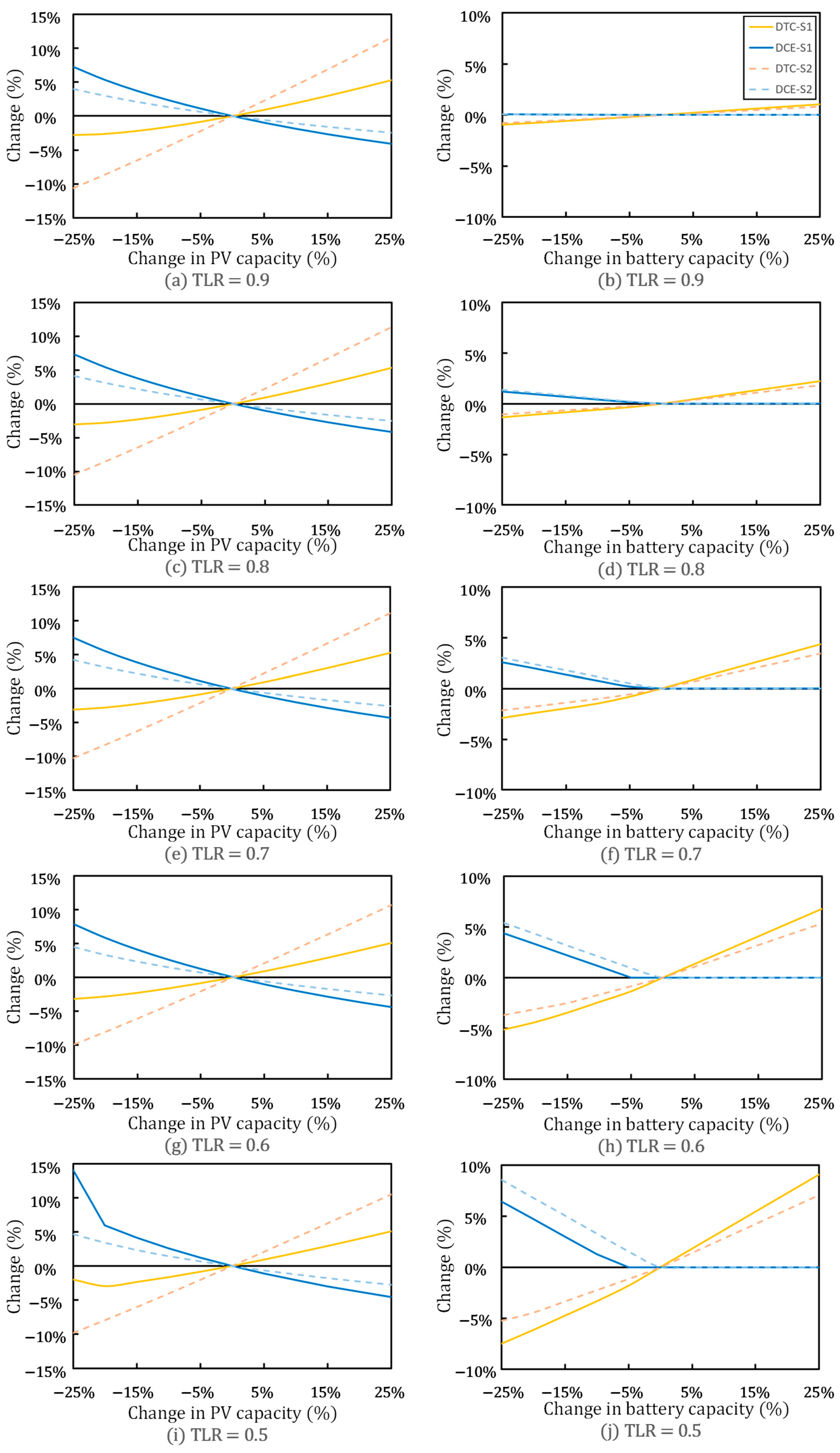
In Figure 20, the influence of variable changes on the objective functions (DTC and DCE) is illustrated. The images on the left describe the impact of changes on the objective functions. The images on the right describe the impact of changes on the objective functions. DTC and DCE changes are represented by yellow and blue, respectively, while scenario 1 and scenario 2 are distinguished by solid and dashed lines, respectively.
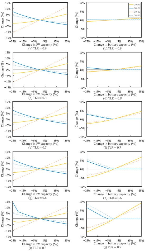
Figure 20.
Effect of change in PV and battery capacity on DTC and DCE.
The system configuration at the origin for is derived from the optimal configuration in Table 6 for , and the data for are similarly derived. Considering that in some configuration cases, the reduced by 25% would be lower than the corresponding , causing the system to be unable to operate safely. Therefore, in this case, insufficient power is assumed to be provided by temporary power supply devices to clearly demonstrate the trend of the changes. Based on Figure 20, the following conclusions can be made:
- The sensitivity curves of for different TLR values are almost identical. The sensitivity curves of are significantly affected by the TLR value; the lower the TLR, the greater the impact on DTC and DCE. When the TLR is high, exerts a stronger influence than on the system’s economic and environmental performance. When the TLR is low (values of 0.6 and 0.5), and have a comparable influence on the system’s performance. Therefore, in practical engineering, when the TLR value is high, the PV configuration is more effective than BESS in improving the performance of the system. When the TLR value is low, the BESS has the same importance as the PV in improving the system performance.
- As shown in Figure 20b,d,f,h,j further increasing the value of will not further reduce DCE. This is because it has already reached the optimal point in terms of energy matching between PV output and power demand. Further increasing will not reduce the power input from the grid to reduce carbon emissions, but will only increase the investment amount. Therefore, in practical engineering, should be configured according to the actual TLR, and to a certain extent, it should be larger than to secure the system’s operational safety, but avoid excessive capacity that causes unnecessary waste.
4.2. Limitations
The study has the following limitations: First, power line loss is not considered in the simulation of the PVB system. This simplification was made to establish a uniform configuration method, but it inevitably introduces a gap between the simulation and reality. Future work should incorporate power line loss to enhance model fidelity. Second, the PVB system was simulated using a predetermined operating strategy. Given that various commonly used strategies exist, each potentially influencing the results, it is imperative to investigate the robustness of the conclusions under different operating strategies.
Finally, while this study successfully demonstrates the multi-objective optimization approach using existing residential buildings as a case study, its applicability to other building types warrants careful consideration. Here, we note that different building types (e.g., offices, shopping malls, restaurants) exhibit distinct load characteristics. The approach, relying on distinct peak and valley load patterns driven by user behavior, is inherently adaptable for scenarios like offices where similar temporal load variations exist (though peak/valley timing may differ) by adjusting model parameters accordingly. However, its effectiveness may be limited for buildings with fundamentally different load profiles, such as industrial facilities characterized by continuous operation and less pronounced demand fluctuations. Therefore, extending and validating the configuration method for diverse building types, including complexes and large industrial parks, represents a necessary direction for future research.
5. Conclusions
PV systems integrated with battery storage are essential for enhancing electrical flexibility in existing urban built environments, particularly in densely populated cities where aging infrastructure and transformer capacity constraints challenge sustainable energy transitions. This study develops a multi-objective optimization approach for PVB systems specifically adapted to existing buildings, effectively balancing energy self-sufficiency improvements while avoiding costly electrical capacity expansions, a critical advantage for rapidly urbanizing regions. The analysis further reveals how capacity allocation decisions directly influence both economic feasibility and environmental outcomes, providing practical guidance for architectural and engineering professionals engaged in building retrofitting projects constrained by grid limitations. By addressing the dual priorities of technical adaptability and sustainability in energy-upgrading existing urban infrastructure, this study contributes actionable strategies to advance decarbonization goals while respecting the operational realities of high-density built environments. The main conclusions are as follows:
- This study employed a residential building in Shanghai as a case study and constructed a mathematical model for the PVB system. The system is operated according to a formulated operational strategy. The TLR is used to express the proportion of to . The simulation results facilitate the analysis of the system domain in a Cartesian coordinate system, where the x-axis represents PV penetration and the y-axis represents TLR. Areas 2 and 3 represent theoretically feasible areas for the PVB system configuration.
- In the domain, the minimum storage capacity () corresponding to each point is calculated, providing constraint conditions for the variable values from the perspective of system safe operation for multi-objective optimization. TLR values have a significant influence on . The lower the TLR value, the larger is the corresponding storage capacity required. In contrast, the effect of on is relatively small. As the increases, the required storage capacity of the system gradually decreases.
- The Pareto optimal set is acquired through the application of the NSGA-II algorithm, with the Diurnal Total Cost (DTC) and Diurnal Carbon Emission (DCE) as the optimization objectives. The weights of the optimization objectives are set based on two scenarios, focusing on economic and environmental performance, respectively, to calculate the optimal configurations for both scenarios. For instance, 0.743 PV penetration and 205 kWh battery are the optimal configurations for economic operation scenarios with the DTC and DCE equal to 367.72 $ and 2940 kgCO2, respectively, when the TLR value is 0.8. For the environmental operation scenario, 1.356 PV penetration, 201 kWh battery is the best optimal configuration with DTC and DCE equal to 444.74 $ and 2667 kgCO2, respectively.
- The impact mechanism of the variables (i.e., A and B under a fixed ) on the system in the optimization method is discussed. When the TLR value is high, the PV configuration is more effective than the BESS in enhancing the system performance. When the TLR value is low, both the PV and BESS have the same importance in improving the system performance. In practical engineering, to guarantee system security, should be configured according to the actual , and to a certain extent, it should be larger than , but avoid excessive capacity that causes unnecessary expenses.
Author Contributions
Conceptualization, J.Y.; Methodology, J.Y. and Y.Z.; Software, J.Y. and Z.Y.; Validation, Y.Z.; Formal analysis, J.Y. and L.C.; Investigation, W.F.; Resources, L.C.; Writing—original draft, J.Y.; Writing—review and editing, Y.Z., Z.Y. and W.F.; Funding acquisition, W.F. All authors have read and agreed to the published version of the manuscript.
Funding
The work was supported by National Natural Science Foundation of China under Grant 52078356; National Key Research and Development Program under Grant 2020YFB21003305; Anhui Province Key Laboratory of Intelligent Building and Building Energy-saving under Grant IBES2022KF12; and Suzhou Municipal Science and Technology Plan Project on Carbon Peak and Carbon Neutrality under Grant ST202313; Fuzhou City Science and Technology Program Project under Grant 2024-Y-002; and Gansu Provincial Department of Housing and Urban-Rural Development Construction Science and Technology Project under Grant JK2024-03.
Data Availability Statement
The original contributions presented in this study are included in the article. Further inquiries can be directed to the corresponding author.
Conflicts of Interest
Author Lie Chen was employed by the company Shanghai Research Institute of Building Sciences Co., Ltd. Author Weidong Fu was employed by the company ARTS Group Co., Ltd. The remaining authors declare that the research was conducted in the absence of any commercial or financial relationships that could be construed as a potential conflict of interest.
Abbreviations
| Acronym: | |
| BESS | Battery energy storage system |
| EV | Electric vehicle |
| NSGA-II | Non-dominated Sorting Genetic Algorithm II |
| PV | Photovoltaic |
| PVB | Photovoltaic battery |
| Scenario 1: economic operation scenario | |
| Scenario 2: environmental operation scenario | |
| List of symbols: | |
| Rated battery capacity (kWh) | |
| minimum battery capacity required (kWh) | |
| CRF | Capital recovery factor (dimensionless) |
| DTC | Diurnal total cost (USD) |
| DCE | Diurnal carbon emission (kgCO2) |
| Electricity consumption of the building load (kWh) | |
| (kWh) | |
| Electricity imported from the utility grid (kWh) | |
| Electricity generated by the PV modules (kWh) | |
| Curtailed electricity generated by the PV modules (kWh) | |
| Available excess PV power generation (kWh) | |
| Operating power of the battery (kW) | |
| Electric power of the building load (kW) | |
| Maximum load power (kW) | |
| Maximum net load power (kW) | |
| (kW) | |
| (kW) | |
| Electric power of the net load (kW) | |
| Electric power imported from the utility grid (kW) | |
| Maximum transmission power (kW) | |
| Generation power of the PV modules (kW) | |
| Curtailed PV power (kW) | |
| PV penetration (dimensionless) | |
| SOC | State of charge (%) |
| TLR | Transmission limit ratio (dimensionless) |
| Unit price of PV (USD/kW) | |
| Unit price of BESS (USD/kWh) | |
| Variable maintenance cost coefficient (USD/kWh) | |
| Fixed maintenance cost coefficient (USD/kWh) | |
| Emission factor of the grid (kg/kWh) | |
References
- Jie, H.; Khan, I.; Alharthi, M.; Zafar, M.W.; Saeed, A. Sustainable energy policy, socio-economic development, and ecological footprint: The economic significance of natural resources, population growth, and industrial development. Util. Policy 2023, 81, 101490. [Google Scholar] [CrossRef]
- Nazari-Heris, M.; Asadi, S. Reliable energy management of residential buildings with hybrid energy systems. J. Build. Eng. 2023, 71, 106531. [Google Scholar] [CrossRef]
- Xiao, Y.P.; Ma, D.L.; Zhang, F.T.; Zhao, N.; Wang, L.; Guo, Z.M.; Zhang, J.; An, B.; Xiao, Y. Spatiotemporal differentiation of carbon emission efficiency and influencing factors: From the perspective of 136 countries. Sci. Total Environ. 2023, 879, 163032. [Google Scholar] [CrossRef]
- Institute, E. Statistical Review of World Energy 2024. 2024. Available online: https://www.energyinst.org/statistical-review (accessed on 30 May 2025).
- Lee, R.; Kim, D.; Yoon, J.; Kang, E.; Cho, H.; Kim, J. Development and calibration of apartment building energy model based on architectural and energy consumption characteristics. Renew. Sustain. Energy Rev. 2024, 206, 114874. [Google Scholar] [CrossRef]
- Del Duca, V.; Ponsiglione, C.; Primario, S.; Strazzullo, S. Towards economic, environmental, and societal sustainable world: Reviewing the interplay of methodologies, variables, and impacts in energy transition models. J. Clean. Prod. 2024, 479, 144074. [Google Scholar] [CrossRef]
- Liu, M.J.; Zhou, C.; Lu, F.F.; Hu, X.H. Impact of the implementation of carbon emission trading on corporate financial performance: Evidence from listed companies in China. PLoS ONE 2021, 16, e0253460. [Google Scholar] [CrossRef]
- Mehmood, U. Contribution of renewable energy towards environmental quality: The role of education to achieve sustainable development goals in G11 countries. Renew. Energy 2021, 178, 600–607. [Google Scholar] [CrossRef]
- Sehar, F.; Pipattanasomporn, M.; Rahman, S. An energy management model to study energy and peak power savings from PV and storage in demand responsive buildings. Appl. Energy 2016, 173, 406–417. [Google Scholar] [CrossRef]
- Huang, B.; Xing, K.; Pullen, S.; Liao, L.D.; Huang, K. Ecological-economic assessment of renewable energy deployment in sustainable built environment. Renew. Energy 2020, 161, 1328–1340. [Google Scholar] [CrossRef]
- Fu, Y.J.; Xu, W.; Wang, Z.C.; Zhang, S.C.; Chen, X.; Chu, J.J. Experimental investigation on thermal characteristics and novel thermal estimation method of BIPV fasade air channel under actual operation. J. Build. Eng. 2023, 72, 106489. [Google Scholar] [CrossRef]
- Sun, H.; Zhu, B.F.; Yin, J.Y.; Zhong, M.T.; Wang, K.Z. Photovoltaic technology in rural residential buildings in China: A comprehensive review on applications, development and its benefits. J. Asian Archit. Build. 2025, 24, 851–865. [Google Scholar] [CrossRef]
- Dong, L.; Liang, H.W.; Gao, Z.Q.; Luo, X.; Ren, J.Z. Spatial distribution of China’s renewable energy industry: Regional features and implications for a harmonious development future. Renew. Sustain. Energy Rev. 2016, 58, 1521–1531. [Google Scholar] [CrossRef]
- Zhao, G.L.; Clarke, J.; Searle, J.; Lewis, R.; Baker, J. Economic analysis of integrating photovoltaics and battery energy storage system in an office building. Energy Build. 2023, 284, 112885. [Google Scholar] [CrossRef]
- Yuan, H.Z.; Ye, H.H.; Chen, Y.T.; Deng, W.Y. Research on the optimal configuration of photovoltaic and energy storage in rural microgrid. Energy Rep. 2022, 8, 1285–1293. [Google Scholar] [CrossRef]
- Pei, N.; Song, X.L.; Zhang, Z.; Peña-Mora, F. Optimizing the operation and allocating the cost of shared energy storage for multiple renewable energy stations in power generation side. Energy Convers. Manag. 2024, 302, 118148. [Google Scholar] [CrossRef]
- Zhang, J.J.; Zhang, J.X.; Skitmore, M.; Ballesteros-Pérez, P.; Zhu, Z.B. Compensation mechanism for peak-shaving auxiliary services considering the cost recovery period of energy storage. J. Energy Storage 2025, 128, 117127. [Google Scholar] [CrossRef]
- Gerber, D.L.; Nordman, B.; Brown, R.; Poon, J. Cost analysis of distributed storage in AC and DC microgrids. Appl. Energy 2023, 344, 121218. [Google Scholar] [CrossRef]
- Hu, Y.; Armada, M.; Sánchez, M.J. Potential utilization of battery energy storage systems (BESS) in the major European electricity markets. Appl. Energy 2022, 322, 119512. [Google Scholar] [CrossRef]
- Nandi, R.; Tripathy, M.; Gupta, C.P. Coordination of BESS and PV system with bidirectional power control strategy in AC microgrid. Sustain. Energy Grids Netw. 2023, 34, 101029. [Google Scholar] [CrossRef]
- Meng, H.; Jia, H.J.; Xu, T.; Wei, W.; Wu, Y.H.; Liang, L.M.; Cai, S.; Liu, Z.; Wang, R.; Li, M. Optimal configuration of cooperative stationary and mobile energy storage considering ambient temperature: A case for Winter Olympic Game. Appl. Energy 2022, 325, 119889. [Google Scholar] [CrossRef]
- Sun, W.Q.; Zhang, J.; Zeng, P.L.; Liu, W. Energy storage configuration and day-ahead pricing strategy for electricity retailers considering demand response profit. Int. J. Electr. Power Energy Syst. 2022, 136, 107633. [Google Scholar] [CrossRef]
- Eskandari, M.; Rajabi, A.; Savkin, A.; Moradi, M.H.; Dong, Z.Y. Battery energy storage systems (BESSs) and the economy-dynamics of microgrids: Review, analysis, and classification for standardization of BESSs applications. J. Energy Storage 2022, 55, 105627. [Google Scholar] [CrossRef]
- Tahir, H.; Park, D.H.; Park, S.S.; Kim, R.Y. Optimal ESS size calculation for ramp rate control of grid-connected microgrid based on the selection of accurate representative days. Int. J. Electr. Power Energy Syst. 2022, 139, 108000. [Google Scholar] [CrossRef]
- Nazir, M.S.; Abdalla, A.N.; Wang, Y.Q.; Chu, Z.; Jie, J.; Tian, P.; Jiang, M.; Khan, I.; Sanjeevikumar, P.; Tang, Y. Optimization configuration of energy storage capacity based on the microgrid reliable output power. J. Energy Storage 2020, 32, 101866. [Google Scholar] [CrossRef]
- Zhu, H.L.; Hou, R.Y.; Jiang, T.T.; Lv, Q.Q. Research on energy storage capacity configuration for PV power plants using uncertainty analysis and its applications. Glob. Energy Interconnect. 2021, 4, 608–618. [Google Scholar] [CrossRef]
- Liang, Z.; Liang, C.; Zhu, W.W.; Ling, L.Y.; Cai, G.W.; Hai, K.L. Research on the optimal allocation method of source and storage capacity of integrated energy system considering integrated demand response. Energy Rep. 2022, 8, 10434–10448. [Google Scholar] [CrossRef]
- Li, S.J.; Zhang, T.; Liu, X.C.; Xue, Z.F.; Liu, X.H. Performance investigation of a grid-connected system integrated photovoltaic, battery storage and electric vehicles: A case study for gymnasium building. Energy Build. 2022, 270, 112255. [Google Scholar] [CrossRef]
- Tan, C.W.; Green, T.C.; Hernandez-Aramburo, C.A. A stochastic method for battery sizing with uninterruptible-power and demand shift capabilities in PV (photovoltaic) systems. Energy 2010, 35, 5082–5092. [Google Scholar] [CrossRef]
- Battal, F.; Balci, S.; Sefa, I. Power electronic transformers: A review. Measurement 2021, 171, 108848. [Google Scholar] [CrossRef]
- Mishra, D.K.; Ghadi, M.J.; Li, L.; Hossain, M.J.; Zhang, J.F.; Ray, P.K.; Mohanty, A. A review on solid-state transformer: A breakthrough technology for future smart distribution grids. Int. J. Electr. Power Energy Syst. 2021, 133, 107255. [Google Scholar] [CrossRef]
- Zhang, Y.; Qian, T.; Tang, W.H. Buildings-to-distribution-network integration considering power transformer loading capability and distribution network reconfiguration. Energy 2022, 244, 123104. [Google Scholar] [CrossRef]
- Teja, S.C.; Yemula, P.K. Architecture for demand responsive HVAC in a commercial building for transformer lifetime improvement. Electr. Power Syst. Res. 2020, 189, 106599. [Google Scholar] [CrossRef]
- Lopes, R.A.; Magalhaes, P.; Gouveia, J.P.; Aelenei, D.; Lima, C.; Martins, J. A case study on the impact of nearly Zero-Energy Buildings on distribution transformer aging. Energy 2018, 157, 669–678. [Google Scholar] [CrossRef]
- Li, C.P.; Zhang, H.; Zhou, H.Y.; Sun, D.P.; Dong, Z.M.; Li, J.H. Double-layer optimized configuration of distributed energy storage and transformer capacity in distribution network. Int. J. Electr. Power Energy Syst. 2023, 147, 108834. [Google Scholar] [CrossRef]
- Hajeforosh, S.; Khatun, A.; Bollen, M. Enhancing the hosting capacity of distribution transformers for using dynamic component rating. Int. J. Electr. Power Energy Syst. 2022, 142, 108130. [Google Scholar] [CrossRef]
- Li, S.B.; Li, X.C.; Kang, Y.Q.; Gao, Q.Y. Load capability assessment and enhancement for transformers with integration of large-scale renewable energy: A brief review. Front. Energy Res. 2022, 10, 1002973. [Google Scholar] [CrossRef]
- Li, Y.S.; Gau, R.H. Transformer-Assisted Deep Reinforcement Learning for Distributed Latency-Sensitive Task Offloading in Mobile Edge Computing. In Proceedings of the ICC 2024-IEEE International Conference on Communications, Denver, CO, USA, 9–13 June 2024; pp. 2944–2949. [Google Scholar] [CrossRef]
- Ding, B.; Li, Z.N.; Li, Z.M.; Xue, Y.X.; Chang, X.Y.; Su, J.; Sun, H. Cooperative Operation for Multiagent Energy Systems Integrated With Wind, Hydrogen, and Buildings: An Asymmetric Nash Bargaining Approach. IEEE Trans. Ind. Inform. 2025. early access. [Google Scholar] [CrossRef]
- Tiwari, R.S.; Sharma, J.P.; Gupta, O.H.; Sufyan, M.A.A. Extension of pole differential current based relaying for bipolar LCC HVDC lines. Sci. Rep. 2025, 15, 16142. [Google Scholar] [CrossRef]
- Qiu, L.; Zhang, H.B.; Zhang, W.R.; Lai, D.Y.; Li, R.X. Effect of existing residential renovation strategies on building cooling load: Cases in three Chinese cities. Energy Build. 2021, 253, 111548. [Google Scholar] [CrossRef]
- Joskow, P.L. Transmission Capacity Expansion Is Needed to Decarbonize the Electricity Sector Efficiently. Joule 2020, 4, 1–3. [Google Scholar] [CrossRef]
- Nagraj, S.M.; Kommadath, R.; Kotecha, P.; Anandalakshmi, R. Multi-objective optimization of vapor absorption refrigeration system for the minimization of annual operating cost and exergy destruction. J. Build. Eng. 2022, 49, 103925. [Google Scholar] [CrossRef]
- Asgari, N.; Saray, R.K.; Mirmasoumi, S. Seasonal exergoeconomic assessment and optimization of a dual-fuel trigeneration system of power, cooling, heating, and domestic hot water, proposed for Tabriz, Iran. Renew. Energy 2023, 206, 192–213. [Google Scholar] [CrossRef]
- Dong, L.L.; Gu, Y.; Cai, K.H.; He, X.; Song, Q.B.; Yuan, W.Y.; Duan, H. Unveiling lifecycle carbon emissions and its mitigation potentials of distributed photovoltaic power through two typical case systems. Sol. Energy 2024, 269, 112360. [Google Scholar] [CrossRef]
- Li, Y.W.; Yang, X.X.; Du, E.S.; Liu, Y.L.; Zhang, S.X.; Yang, C.; Zhang, N.; Liu, C. A review on carbon emission accounting approaches for the electricity power industry. Appl. Energy 2024, 359, 122681. [Google Scholar] [CrossRef]
- Kaabeche, A.; Belhamel, M.; Ibtiouen, R. Sizing optimization of grid-independent hybrid photovoltaic/wind power generation system. Energy 2011, 36, 1214–1222. [Google Scholar] [CrossRef]
- Diaf, S.; Notton, G.; Belhamel, M.; Haddadi, M.; Louche, A. Design and techno-economical optimization for hybrid PV/wind system under various meteorological conditions. Appl. Energy 2008, 85, 968–987. [Google Scholar] [CrossRef]
- Zhang, L.H.; Wang, S.; Ni, Z.H.; Li, F.S. Maximum power point tracking control of photovoltaic systems using a hybrid improved whale particle swarm optimization algorithm. Energy Sources Part A 2025, 47, 1789–1803. [Google Scholar] [CrossRef]
- Li, S.J.; Zhang, T.; Liu, X.C.; Liu, X.H. A Battery Capacity Configuration Method of a Photovoltaic and Battery System Applied in a Building Complex for Increased Self-Sufficiency and Self-Consumption. Energies 2023, 16, 2190. [Google Scholar] [CrossRef]
- Ayeng’o, S.P.; Axelsen, H.; Haberschusz, D.; Sauer, D.U. A model for direct-coupled PV systems with batteries depending on solar radiation, temperature and number of serial connected PV cells. Sol. Energy 2019, 183, 120–131. [Google Scholar] [CrossRef]
- Hou, Q.C.; Zhang, N.; Du, E.S.; Miao, M.; Peng, F.; Kang, C.Q. Probabilistic duck curve in high PV penetration power system: Concept, modeling, and empirical analysis in China. Appl. Energy 2019, 242, 205–215. [Google Scholar] [CrossRef]
- Li, H.; Zhang, J.; Liu, X.H.; Zhang, T. Comparative investigation of energy-saving potential and technical economy of rooftop radiative cooling and photovoltaic systems. Appl. Energy 2022, 328, 120181. [Google Scholar] [CrossRef]
- Yan, Z.; Zhang, Y.M.; Yu, J.S.; Ran, B.W. Life cycle improvement of serially connected batteries system by redundancy based on failure distribution analysis. J. Energy Storage 2022, 46, 103851. [Google Scholar] [CrossRef]
- May, G.J.; Davidson, A.; Monahov, B. Lead batteries for utility energy storage: A review. J. Energy Storage 2018, 15, 145–157. [Google Scholar] [CrossRef]
- Jing, R.; Zhu, X.Y.; Zhu, Z.Y.; Wang, W.; Meng, C.; Shah, N.; Li, N.; Zhao, Y. A multi-objective optimization and multi-criteria evaluation integrated framework for distributed energy system optimal planning. Energy Convers. Manag. 2018, 166, 445–462. [Google Scholar] [CrossRef]
- Gouareh, A.; Settou, B.; Settou, N. A new geographical information system approach based on best worst method and analytic hierarchy process for site suitability and technical potential evaluation for large-scale CSP on-grid plant: An application for Algeria territory. Energy Convers. Manag. 2021, 235, 113963. [Google Scholar] [CrossRef]

Disclaimer/Publisher’s Note: The statements, opinions and data contained in all publications are solely those of the individual author(s) and contributor(s) and not of MDPI and/or the editor(s). MDPI and/or the editor(s) disclaim responsibility for any injury to people or property resulting from any ideas, methods, instructions or products referred to in the content. |
© 2025 by the authors. Licensee MDPI, Basel, Switzerland. This article is an open access article distributed under the terms and conditions of the Creative Commons Attribution (CC BY) license (https://creativecommons.org/licenses/by/4.0/).