Abstract
Power transformers are a key piece of equipment located between the points of supply and consumption of electrical energy. Due to their continuous exposure to the environment, they may be subject to failure. Thus, the modeling of transformers subject to incipient faults using a bond graph approach is presented in this study. In particular, incipient faults in the primary and secondary windings with respect to ground and a turn-to-turn fault in the primary winding are modeled. In order to develop a mathematical model capturing the incipient faults in transformers including magnetic saturation effects, a junction structure for the system applied to the bond graph model is proposed. The steady-state responses of the faulted transformer models using a bond graph approach are presented, leading to the proposal of a method for fault analysis in transformers with DC supply sources. Simulation results for the transformers with the different faults are presented, validating the results obtained according to expressions derived from the bond graph models.
1. Introduction
Electrical power transformers are fundamental elements in an electrical power system which link the generation, transmission, and distribution stages of electrical energy under different voltages and currents. However, transformers are susceptible to failure, mainly due to their exposure to adverse environmental conditions. Thus, the modeling of transformers with incipient faults for analysis of their condition has led to interesting and vital studies in the field of electrical engineering.
Some models have been developed for the study of transformers with incipient faults in their windings. One essential model is the transformer with incipient faults proposed in [1]. Another was presented in [2]. Subsequently, numerous works have been published on different aspects of transformers with this type of failure, among which the following can be mentioned:
The monitoring of variables of a transformer for the detection and identification of faults has been proposed in [3]. Predictive models for the detection of incipient failures in transformers were developed in [4]. The transient response of a winding with an inter-turn discharge was simulated using a finite element model and its mechanical effect on a three-phase transformer was analyzed in [5]. A diagnostic model for incipient transformer faults using artificial neural networks was developed in [6]. A method for modeling incipient faults in single-phase transformers that is compatible with the ATP software has been presented in [7]. A computational and experimental study of magnetic and electrical variables for the detection of incipient faults in transformers was reported in [8]. Computational models for the simulation of incipient transformer failures have been developed in [9].
A scalable design for the simulation of winding failures in three-phase transformers using numerical statistical methods was investigated in [10]. A new S-transform (ST) for the protection of transformers with incipient faults was proposed in [11]. A learning system which can be applied for the recognition of internal faults in miniature transformers was presented in [12]. The injection current to a power transformer required to assess an internal fault and the behavior of the differential relay was analyzed in [13]. Fault detection in power transformers using fuzzy logic and neural networks has been discussed in [14]. A multi-layer artificial neural network to identify incipient faults in transformers was proposed in [15]. The diagnosis of incipient faults in power transformers using fuzzy logic was proposed in [16].
Online monitoring of the instantaneous exciting current space phasor in transformers allows for the detection of inter-turn faults, as proposed in [17]. An intelligent expert system for the diagnosis of faults in power transformers was applied in [18]. A review and analysis (including challenges and future directions) regarding the detection of incipient failures in power distribution networks was developed in [19]. Vibration frequency analysis for the detection of inter-turn faults in transformers as a novel approach was proposed in [20]. The modeling and simulation of a three-phase transformer in Matlab for monitoring purposes was developed in [21]. The modeling of three-phase transformers under internal fault conditions and the behavior of the magnetizing current were analyzed in [22]. The use of machine learning approaches to interpret data on incipient failures in power transformers has been discussed in [23]. The application of the hyperbolic S-transform to detect incipient faults in transformers was proposed in [24].
The bond graph methodology was introduced by Paynter in 1961. Subsequently, researchers such as Karnopp, Rosenberg, Thoma, Brown, and Breeveld have published numerous advances in papers and books that comprise the state of the art regarding the modeling and application of bond graphs. A bond graph determines the formal and unified procedures in the modeling of dynamic physical systems. One of the main characteristics of a bond graph is the ability to analyze the exchange of power between its elements. This unified character allows for the modeling of systems comprising several energy domains (electrical, mechanical, hydraulic, magnetic, thermal). Likewise, the structural properties of systems—such as their stability, observability, controllability, and steady-states—can be derived almost directly from systems modeled as bond graphs. In addition, bond graphs have been extended for control design activities. To date, bond graph modeling has been widely used to obtain new procedures for the structural analysis of systems [25], model reduction [26,27], as well as the development of system modeling software [28]. Systems modeled using bond graphs can be linear or non-linear, and time-variant or time-invariant. Essential references on modeling with and the properties of bond graphs include [29,30,31]. However, recent advances in bond graph theory comprise various directions, as detailed below.
A non-linear transformer model using a bond graph approach to understand the energy exchanges in a traction chain and perform parameter identification was studied in [32]. A method for converting electrical circuits to their bond graph equivalent for modeling and simulation in SPICE was proposed in [33]. The use of bond graphs as tools in control theory for mechatronics students and for the design of a PID controller was discussed in [34]. A bond graph model representing a virtual model of the mechanical and hydraulic interconnections in Rough-Terrain Variable Reach Trucks was presented in [35]. The fault diagnosis of a three-phase induction motor using a bond graph and a time causal graph was proposed in [36]. A dynamic model of an isolator was obtained from the associated bond graph, and the energy transfer characteristics were found in [37].
The use of a bond graph representing a thermal system (incubator) to localize an industrial system according to analytical redundant relationships and applying linear fractional transformations was proposed in [38]. The bond graph approach was applied for the modeling of biochemical systems with feedback control, allowing biochemical oscillators to be obtained [39]. The heat transferred from fuel rods to the coolant is a generic process in a nuclear reactor, which has been represented as a pseudo-bond graph and combined with a Petri net for analysis of the impacts of temperatures in [40]. Various applications of bond graphs in the fields of biology and physiology have been reviewed in [41].
In this study, a model of an electrical power transformer using a bond graph-based approach, considering the effects of magnetic saturation, is proposed. Due to the characteristics of the model, a junction structure is proposed for this class of non-linear systems to obtain a mathematical model of the considered system. The obtained model is then used to analyze incipient faults in the primary and secondary windings of the transformer. For each of the applied faults, a mathematical model of the system is obtained. In this way, a structural analysis of the transformer under fault conditions can be performed.
The steady-state response of a system is an interesting characteristic of its behavior under nominal conditions. Thus, the steady-state responses of the transformer under fault conditions and constant supply sources are obtained. As these results allow us to determine the operating conditions of the transformer, it is proposed to include these test results to obtain the transformer status with a DC voltage supply source. Simulations of transformers with and without faults are performed using the 20-Sim software.
Bond graph modeling allows for the analysis of linear and non-linear dissipation and storage elements, as well as elements formed by different energy domains. Therefore, this study provides a basis for modeling transformers, including the effects of the filling liquid and taking into account magnetic–electric transduction, thus enabling analysis of the structural properties of stability, controllability, observability, and linearity at different time scales, along with their implications under the applied incipient faults.
The main contributions of this study are the following:
- A bond graph model of the transformer is presented, including magnetic saturation effects.
- A junction structure of this class of non-linear systems is proposed for determination of a mathematical model from the bond graph in integral causality (BGI).
- A junction structure for obtaining the steady-state response from a bond graph in derivative causality (BGD) is proposed.
- Bond graph models of the transformer with incipient faults in the primary and secondary windings and their mathematical models are presented.
- Steady-state responses under fault conditions from the respective BGD models are detailed.
- A fault analysis approach for transformers with incipient faults and constant voltage sources is proposed.
Section 2 describes the essential elements in bond graph modeling, with an emphasis on electrical systems. Likewise, junction structures for the BGI (dynamic equations) and BGD (steady-state) models are proposed for this class of non-linear systems. Traditional models of electrical transformers are summarized in Section 3, and a bond graph model considering magnetic saturation effects is proposed. Section 4 describes the modeling of incipient faults in transformers, as well as the associated dynamic model and steady-state responses. The simulation results are presented in Section 5.
2. System Modeling with Bond Graphs
A bond graph is a system modeling methodology based on the transfer of power between its elements. The fundamental elements of bond graphs are the power bonds, as shown in Figure 1. Two generalized power variables are associated with each bond, called the effort and flow which, for electrical systems, correspond to the voltage and current , respectively [29,30,31].
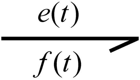
Figure 1.
Power bond.
In particular, the product of these variables determines the power flow:
Associated with the power variables, we have two generalized energy variables called the moment and displacement
An essential property in bond graph modeling is causality, which allows one to determine the direction of effort and flow, as shown in Figure 2.
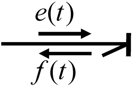
Figure 2.
Causal bond.
The set of elements required to build a bond graph model of an electrical system is described below [29,30,31].
The power supply sources (called port-1 active elements) are indicated in Figure 3.
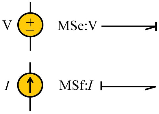
Figure 3.
Power sources in bond graph.
The electrical resistances are modeled as port-1 passive elements, as shown in Figure 4.
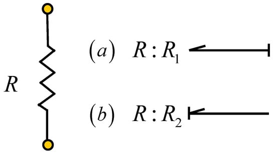
Figure 4.
Resistance in a bond graph.
Depending on the causality (Figure 4a,b), constitutive relations for the resistance are given by and .
The inductances are modeled according to Figure 5.
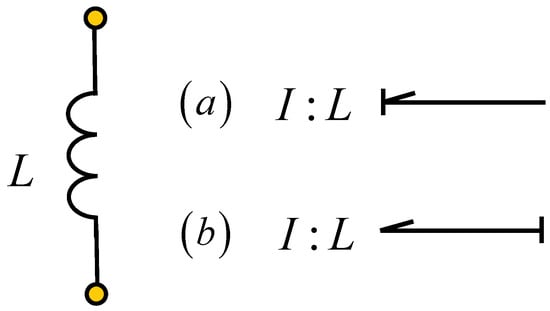
Figure 5.
Inductance in a bond graph.
The application of causality to this storage element determines an integral causality assignment for Figure 5a, with a non-linear constitutive relationship for the linear case , where the relationship between the input variables and the output variable is defined by mathematical integration.
For the case in Figure 5b, the non-linear constitutive relationship is ; for the linear case, . Note that the relationship between the variables is the mathematical derivative and, so, derivative causality is assigned to this storage element.
The capacitor elements are modeled according to Figure 6.
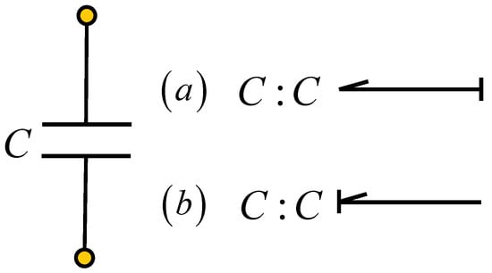
Figure 6.
Capacitance in a bond graph.
The assignment of integral causality to this element is drawn according to Figure 6a, with the non-linear constitutive relationship given by for the linear case . Note that the relationship between the variables here is defined by mathematical integration.
For Figure 6b, the non-linear constitutive relationship is expressed by for the linear case , where the relationship between the variables is mathematical derivation.
Another important type of element in bond graph modeling is the port-2 element. The transformer is one of these elements formed by two bonds, as shown in Figure 7.
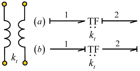
Figure 7.
Transformer in a bond graph.
For Figure 7a, the constitutive relations are defined by and ; meanwhile, for Figure 7b, we have and .
Another port-2 element is the gyrator illustrated in Figure 8.
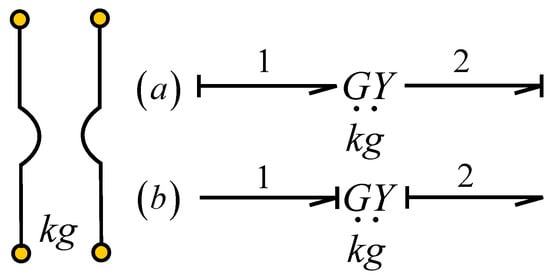
Figure 8.
Gyrator in a bond graph.
The constitutive relations for Figure 8a are described by and ; meanwhile, for the case of Figure 8b, we have and .
Finally, the interconnection elements in bond graph are called 3-ports or junctions. A 1-junction represents a series connection while a parallel connection is represented by a 0-junction, as shown in Figure 9.
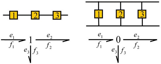
Figure 9.
Serial and parallel connections in a bond graph.
The constitutive relations for serial connections are described by and ; meanwhile, those for parallel connections are described by and
2.1. Mathematical Model Derived from a Bond Graph
Once a model of a system has been obtained in the form of a bond graph, the next stage is to determine the mathematical model. Transformers are electrical systems that can be modeled as linear systems; however, when the effect of magnetic saturation is considered in the magnetization branch, transformer models represent a class of non-linear systems. Therefore, a block diagram of a bond graph model is proposed as an approximation of transformers with linear and non-linear storage elements, as shown in Figure 10.
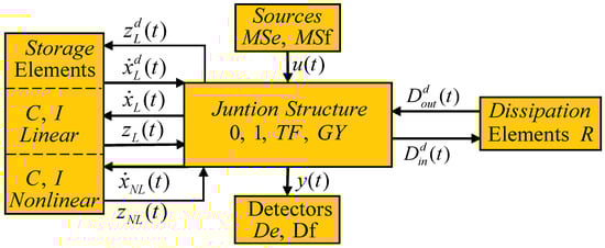
Figure 10.
Junction structure of a class of non-linear systems.
The junction structure of Figure 10 is formed by the following:
- The source field , which supplies the input power to the system with the key vector .
- The detection field , which determines the output of the system through the vector .
- The dissipation field , which brings together the elements that dissipate power. This energy exchange is given by and .
- The storage field , which forms the inductances and capacitances for an electrical system, and can be linear with vectors or non-linear with vectors , these elements being linear with respect to the coenergy elements and . In this field, linearly dependent elements can be considered as key vectors and
- The junction structure , containing 0- and 1-junctions, transformers, and gyrators.
The mathematical model of the system shown in Figure 10 is obtained according to the following lemma.
Lemma 1.
Consider a class of non-linear systems represented by a bond graph model with predefined integral causality assignment in its storage elements whose key vectors are defined according to Figure 10, where the junction structure is defined by
with the constitutive relations of the storage elements given by
and, for the dissipation elements,
Then, the state-space model is described by
with output
where
with
Proof.
The relationship of the linear storage elements in integral and derivative causality is obtained from the fourth line of (2) along with (3) and (5),
starting from the third line of (2) with (6),
replacing (22) and (21) in the first line of (2) with (3) and (4),
Factoring from (23) with (10), (12), and (14), the state Equation (7) is proven.
Substituting (22) in the second line of (2) with (3) and (4),
from (24) with (11), (13), and (15), the state equation for non-linear elements (8) is proven.
For the output equation from the fourth line of (2) with (22) and (6),
from (25) with (16)–(18), the output Equation (9) is proven. □
2.2. Steady-State Response from a Bond Graph
The dynamic responses of a system describe the evolution of its variables over time. However, when the transient stage ends, only steady-state magnitudes are available. For an LTI system, the steady-state model is determined from
Applying in (26) and (27),
where , , and are the steady-state responses of the state variables, the output, and the input, respectively.
For the system considered in this paper defined by (7)–(9), it is not easy to determine the steady-state response from (28) and (29) due to the non-linear component. In the analysis of systems represented as bond graphs, the determination of this response from a bond graph in derivative causality (BGD) has been proposed, where storage elements are assigned derivative causality [42]. In this paper, this result is extended to the system defined by (7)–(9), for which the analysis of a bond graph in derivative causality is proposed according to the block diagram shown in Figure 11.
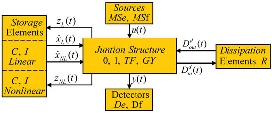
Figure 11.
Bond graph in derivative causality.
In the BGD of a system, it is not only required that the storage elements be assigned derivative causality but also that the causality of the junctions be adjusted such that the bond graph is correct; generally, this means that the causality of dissipating elements is changed. Thus, in the BGD, there are key vectors between the dissipative elements and the junction structure defined by and which are generally different than and in the corresponding BGI.
In this paper, the steady-state response in a bond graph approach for the given system in (7)–(9) is obtained according to the following lemma:
Lemma 2.
Consider a class of non-linear systems modeled as a bond graph with all storage elements in derivative causality, according to Figure 11, whose junction structure is defined by
with constitutive relations given by (3), (5) and for the dissipation elements
Then, the steady-state of the state variables and the output of the system are described by
where
and is the steady-state of the input .
Proof.
From the third line of (30) with (31),
Replacing (39) in the first line of (30) with (31),
and using (38) in (40),
This expression can be reduced to
where
with as defined in (35). The state space representation of the system in BGD given in (42) allows us to obtain the steady-state of the linear state variables by setting and . Thus, (32) is proven.
Starting from the second line of (30) with (39) and (31),
Substituting (38) in (45),
can be described as
where
and is defined in (36). Setting and , it is proven that the steady-state of the non-linear state variables is given by (33).
From the third line of (30) with (39) and (31),
With (38), this reduces to
which can also be expressed by
where
with as defined in (37). Setting and in (52), then (34) is proven. □
3. Model of a Two-Winding Transformer
Steinmetz developed the circuit model that is universally used for the analysis of iron-core transformers at various power frequencies. His model has many advantages over those resulting from the straightforward application of linear circuit theory, primarily because the iron core exhibits saturation and hysteresis and is, thus, definitely non-linear [43]. Consider the magnetic coupling between the primary and secondary windings of a transformer shown in Figure 12 [43].
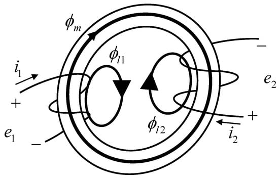
Figure 12.
Magnetic coupling of a two-winding transformer.
The total flux linkage of each winding is defined by two components: the mutual magnetic flux and the flux linkage of each winding and . In terms of these flux components, the total flux for each of the windings can be expressed as
Assuming that turns of winding 1 effectively link and , the flux linkage of winding 1 is defined by
The leakage and mutual fluxes can be expressed in terms of the winding currents using the magneto-motive forces (mmfs) and permeances. Thus, the flux linkage of winding 1 is
where and .
Similarly, the flux linkage of winding 2 can be expressed as
and, using the mmfs and permeances for this winding,
The resulting flux linkage equations for the two magnetically coupled windings, expressed in terms of the winding inductances, are
where and are the self-inductances of the windings, and and are the mutual inductances between them.
Note that the self-inductance of the primary winding can be divided into two components—the primary leakage inductance and the primary magnetizing inductance —which are defined by
where and .
Likewise, for winding 2,
where and .
Finally, the mutual inductance is given by
Taking the ratio of to ,
The induced voltage in winding 1 is given by
Replacing by and by we obtain
Similarly, the induced voltage of winding 2 can be written as
Finally, the terminal voltage of a winding is the sum of the induced voltage and the resistive drop in the winding. The complete equations for the two windings are
where .
Bond graph modeling allows one to obtain a simple and direct model of the system from which mathematical models, structural analysis, and controller design scopes can be derived, according to the needs of the system. Thus, according to the essential elements in the bond graph modeling of electrical systems, a bond graph of a transformer is shown in Figure 13.
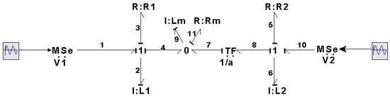
Figure 13.
Bond graph of a transformer.
In Figure 13, we have the primary winding circuit whose parameters are , denoting resistance, inductance, and voltage, respectively; for the secondary winding, are the resistance, inductance, and voltage connected to this circuit; denote the magnetization inductance and the losses in the core; and a is the transformation ratio. Thus, the key vectors in the BGI of the transformer are described by
with constitutive relations
The junction structure of the transformer can be expressed as

The mathematical model of the transformer for the linear state variables that represent the primary and secondary windings is obtained by substituting (71)–(74) into (26) with (10), (12), and (14), which produces
Furthermore, from (11), (13), (73), and (15) with (71), (72), and (74), the state equation for the non-linear variable representing the magnetizing inductance is given by
The analysis of incipient failures can be performed with the modeled transformer, as detailed in the next section.
4. Bond Graph of a Transformer with Incipient Faults
The degradation of the insulation in the conductors used to form the windings of a transformer leads to incipient failures. A voltage is applied in the operation of a transformer, producing a high electric field in the dielectric of the conductors of the windings which can cause deterioration of the insulation. This deterioration is mainly due to thermal, electrical, and mechanical stress factors.
Thermal stresses occur with internal heating due to current overloads. Voltage changes in the insulation produce electrical stresses. Mechanical stresses occur due to assembly, manufacturing techniques, and vibrations. The decrease in dielectric properties is mainly due to humidity.
The electrical behavior of a dielectric material can be modeled in a traditional way with an equivalent parallel circuit, as shown in Figure 14.
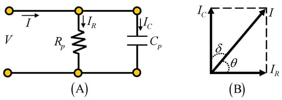
Figure 14.
Equivalent model of a dielectric material: (A) equivalent circuit; (B) phasor diagram of the circuit.
In Figure 14, V is the applied voltage and I is the current through the isolation with the components through the capacitor and through the resistance. R represents the losses in the dielectric part and C is the capacitance of the dielectric material. In the phasor diagram shown in Figure 14B, is the angle due to losses and is called the loss tangent or the dissipation factor. The calculation of cos θ yields the power factor of the dielectric. The dissipation factor can be expressed as
and the energy dissipated as heat in the dielectric is proportional to (77).
According to (77), it is common to analyze the behavior of incipient failures to consider given values of w and and vary the value of to obtain , as indicated in Table 1.

Table 1.
Circuit parameters of the dielectric material.
4.1. Fault in Primary Winding to Ground
Firstly, the incipient failure model shown in Figure 14 is applied to the primary winding of a single-phase power transformer, as illustrated in Figure 15. Due to the faulty transformer connection, the winding is divided into two parts, , where section denotes the number of turns in which the fault is present and is the number of turns in the section without failure, while is the number of turns of the secondary winding. The voltages applied to the primary and secondary windings are and , respectively.
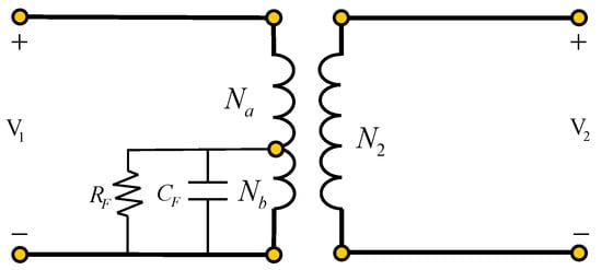
Figure 15.
Transformer with primary winding to ground fault.
The bond graph in integral causality for the primary winding to ground fault model is shown in Figure 16. This bond graph is obtained from the bond graph of the transformer in Figure 16 and, due to the partition of the primary winding due to the fault, there are two transformation relations and a.
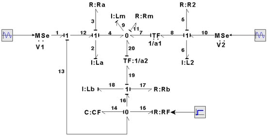
Figure 16.
BGI of transformer with primary winding to ground fault.
The key vectors of this bond graph are
and the constitutive relations are defined by
while the junction structure is given by

In this case, if there are no storage elements in derivative causality, then . From (10), (79), (80), and (82), the state matrix of the linear storage elements is described by
Substituting (82) in (12) with (81), the non-linear state matrix reflected in the linear states is given by
and the input matrix is obtained from (82) in (14):
Then, with (83)–(85), the mathematical model of linear elements is
From (11), (13), (15) with (79)–(82), the state matrix for the non-linear element is expressed by
The steady-state response in a bond graph approach requires obtaining the bond graph in a derivative causality assignment of the storage elements, according to Lemma 2. For this fault, the corresponding BGD is shown in Figure 17.
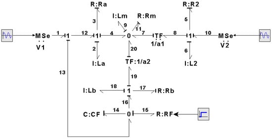
Figure 17.
BGD of transformer with primary winding fault.
The key vectors that are modified in the BGD are those related to the dissipation field; thus,
its constitutive relationship being expressed by
The junction structure for this BGD is defined by

As the submatrix , from (38), (89), and (90), we have
where
The steady-state is obtained by substituting (90) and (91) into (35) and (32), which is given by
Substituting (90) and (91) into (36) and (33) for the non-linear element, we obtain
4.2. Fault in the Secondary Winding to Ground
The next fault to be modeled is located in the secondary winding to ground, as shown in Figure 18. In this case, the secondary winding has been divided into , which represents the number of turns in the section of the winding with no fault, and is the number of turns in the part where the fault is located.
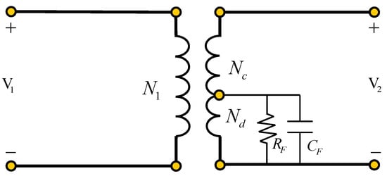
Figure 18.
Secondary winding to ground fault.
The bond graph for this fault is illustrated in Figure 19.
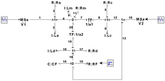
Figure 19.
BGI for secondary winding to ground fault.
When considering the same transformer but with an incipient fault in the secondary winding to ground, the key vectors are the same as for the fault in the primary winding expressed by (78), with the constitutive relations
and (81), with the junction structure for this BGI being described by

From (10), (12), (14) with (81), (95)–(97), the state equation for the linear elements is defined by
The state equation for the non-linear element is obtained by substituting (79)–(81), and (97) in (11), (13), and (8), which can be described as
The corresponding BGD for this transformer fault is illustrated in Figure 20.
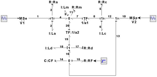
Figure 20.
BGD of transformer with secondary winding fault.
The key vectors of the BGD in Figure 20 are the same as those for the BGD in Figure 19; therefore, the junction structure is defined by

In this case, the matrix N is obtained from (38), (89), and (100) as
where
Substituting (100) and (101) into (35) and (32), the steady-state at this failure condition is expressed by
Substituting (100) and (101) into (36) and (33), the steady-state of the non-linear element is obtained as
4.3. Inter-Turn Fault in the Primary Winding
Another type of failure that can happen in a transformer is an inter-turn failure, which, in this study, is modeled in the primary winding. The schematic diagram of this fault is shown in Figure 21. In this case, the faulted winding is divided into three subsections of the primary winding , with respective numbers of turns , , and .
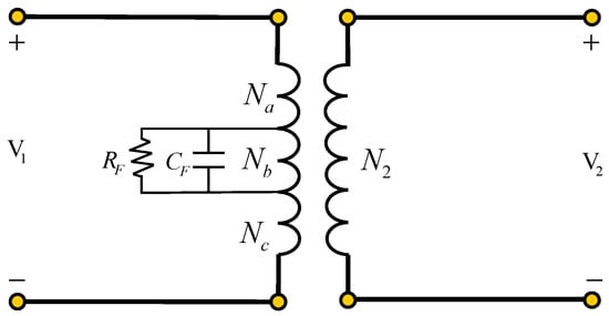
Figure 21.
Inter-turn fault in the primary winding.
The BGI of this transformer with the inter-turn fault in the primary winding is illustrated in Figure 22, in which there are three terms, reflecting the sections that appear in the failed winding.
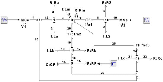
Figure 22.
BGI of the transformer with a fault between turns in the primary winding.
As the primary winding is divided, the key vectors are similar to the previous cases but present certain differences. The key vectors for are as defined in (78); however, and are given by
The constitutive relations for these key vectors (105) are defined by
and the junction structure is described as follows:
 where
where
In this case, we have a storage element in derivative causality. Thus, from (19), (79), (107), and (108), the relationship between this element and the linearly independent element is expressed by
From (10), (12), (14) with (79), (106), and (108),
From (11), (13), (15) with (79), (106), and (108), the state equation for the non-linear element is given by
The steady-state response under this failure condition requires the BGD shown in Figure 23.
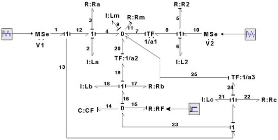
Figure 23.
BGD of the transformer with inter-turn fault in the primary winding.
The key vectors for the dissipative elements of the BGD are
with
The junction structure for the BGD is
 where
where and .
where
where and .
Substituting (113), (114), and (115) in (35) and (32), the steady-state of linear elements is
From (113), (114), and (115) in (36) and (33), the steady-state for the non-linear element is determined by
5. Simulation Results
Before presenting the simulations of the transformers with incipient faults, it is interesting to describe the behavior of the transformer with a non-linear magnetization inductance in order to analyze the currents in the system windings. The numerical parameters of the transformer are detailed in Table 2.
Table 2.
Transformer.
The non-linear function of the magnetization impedance is defined by [44]
with . The values of the non-linear function (i.e., 0.8642 and 0.3215) are calculated according to the excitation current required by the transformer. Due to the characteristics of the bond graph model, the type of core is not taken into account and no changes are made in the frequency of the supply voltages.
The first part of the simulation results utilizes the two supply voltages to the transformer shown in Figure 24.
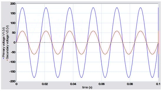
Figure 24.
Supply voltages to the transformer.
The behaviors of the primary and secondary windings are illustrated in Figure 25.
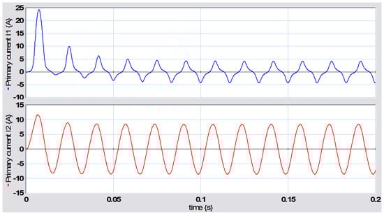
Figure 25.
Currents in the primary and secondary windings.
Note that the current in the primary winding presents a distortion because the transformer is operating in the magnetic saturation region and reaches a maximum value of 24.27 A, with the nominal time constant of the primary winding being mH/2.9 ms. The current in the excitation branch with respect to the flux links in the magnetization inductance gives rise to the hysteresis phenomenon shown in Figure 26.
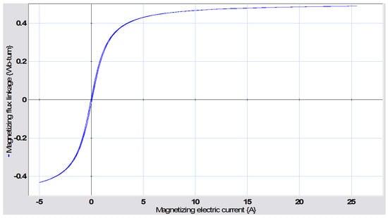
Figure 26.
Hysteresis in the transformer.
According to the transformer hysteresis graph in Figure 26, it can be clearly seen that the current in the primary winding is distorted by the effect of magnetic saturation while the current in the secondary winding presents the common form of a sinusoidal wave.
5.1. Primary to Ground Fault
The first fault applied to the transformer is in the primary winding with respect to ground. Based on references to incipient faults in transformers [2], the equivalent capacitance presents small changes under fault conditions and, considering the data in Table 2 and F and changing , the different values of under various failure scenarios were obtained. Thus, the resistance initially has a value of while, at a time of s, s changes to when an incipient fault is applied. If the fault applies to the winding at turn 350, then and . Applying these turn ratios to the resistances and inductances, the following values were obtained: , mH, and mH. The simulation results for this fault are shown in Figure 27.
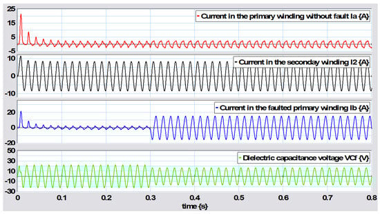
Figure 27.
Simulation of fault in the primary winding to ground.
It can be seen that at the moment the fault appeared at s, the current in the fault winding section presented a sudden increase produced by the fault, which can be seen to have occurred within a short time range in Figure 28.
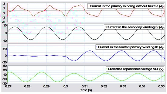
Figure 28.
Primary failure in a range of s to s.
The transformer was then analyzed with a fault condition in the primary winding and a parametric disturbance of the inductance in section a in this winding, which starts at s and ends at s with a value of H. This behavior can be seen in Figure 29.
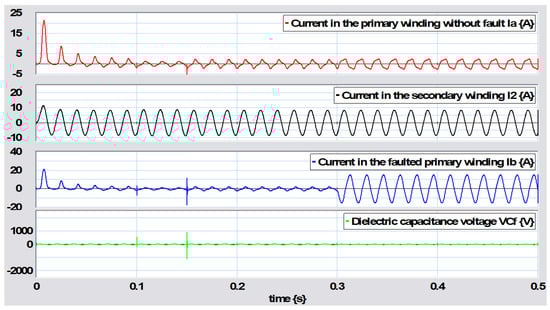
Figure 29.
Transformer behavior with parametric disturbance over a wide time range.
Figure 30 shows the behaviors of the variables under parametric change of the inductance.
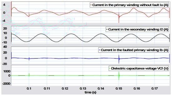
Figure 30.
Behaviors observed during parametric change.
Notably, the changes are not very clear, except that the magnitudes changed. Therefore, Figure 31 better illustrates the transient occurring when this parametric change in inductance ended.
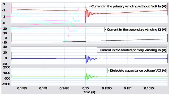
Figure 31.
Transient due to a parametric disturbance.
Considering the behavior of the transformer with a fault in the primary winding and an external disturbance applied to the voltage in the primary winding, the obtained results are shown in Figure 32.
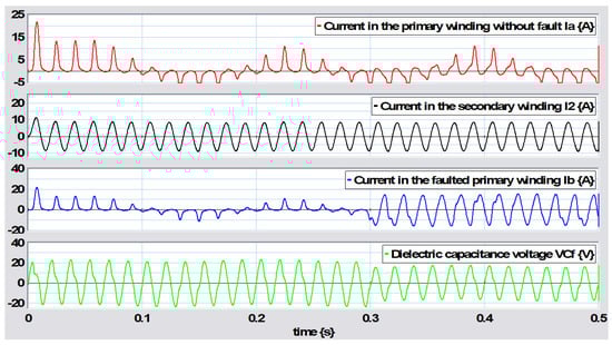
Figure 32.
Transformer behavior with a primary fault and a low−frequency disturbance voltage.
In particular, the external disturbance is a low frequency of 6 Hz. Next, applying a disturbance voltage with a frequency of 600 Hz and a maximum value of 30 V V, the resulting behavior is shown in Figure 33.
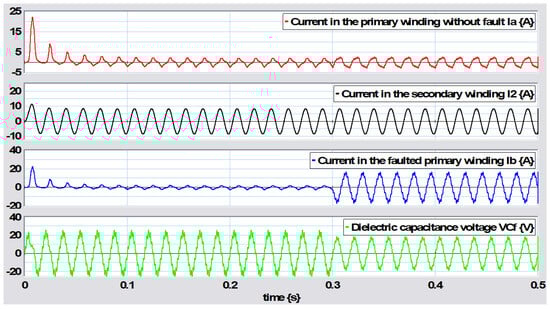
Figure 33.
Transformer behavior with a primary fault and a high−frequency disturbance voltage.
In order to validate the expressions obtained from the steady-state response, we consider the use of direct current sources; namely,
Substituting the numerical values in the steady-state response of (93), we obtain the values without failure as
With an incipient failure with ,
These values can be verified from the graphs shown in Figure 34.
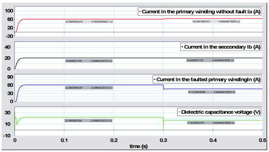
Figure 34.
Steady−state response with respect to primary winding to ground fault.
Figure 34 shows that the fault in the primary winding can be monitored from current measurements at the beginning of winding or at the end . However, the current sensor in showed only a slight change, such that it might not be very effective in that section of the winding, while indicated that the large change in current caused a fault.
5.2. Secondary Winding to Ground Fault
Next, an incipient fault was applied in the secondary winding of the transformer with the numerical values shown in Table 2 and F. Initially, the transformer operates without failure with . At a time of s, the fault is applied with . This fault is applied to the winding at the number of turns , and spans . The parameters for this fault are , , mF, and mH. The dynamic behavior of the transformer in this operating condition is shown in Figure 35.
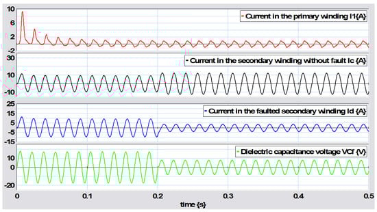
Figure 35.
Fault in the secondary winding with respect to ground.
Analyzing this fault in the secondary winding in a time range close to the fault point at s, the resulting behavior is shown in Figure 36.
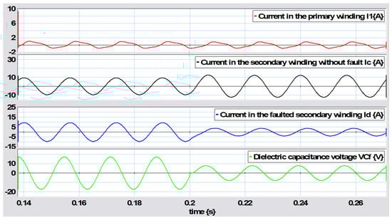
Figure 36.
Secondary winding failure within a short time range.
In this fault, a large change in current can be seen in the section reflecting of the secondary winding of the transformer and, so, it is evident that the fault that occurred is detected. The numerical results for the steady-state are obtained by substituting (119) in (103) with before failure, which are
When the failure happens, ,
The steady-state analysis of the transformer with a fault in the secondary winding is illustrated in Figure 37, verifying the values given in (122) and (123).
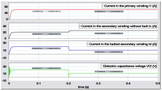
Figure 37.
Failure in the secondary winding with the BGD.
Figure 37 indicates the presence of a fault in the secondary winding, with a notable change in the magnitudes of the currents and when the fault occurs at s.
5.3. Failure Between Turns in the Primary Winding
The behavior of the transformer when a fault occurs in the primary winding between turns is shown in Figure 38, with the failure occurring at a time of s. Note that the currents in the three sections into which the primary winding has been divided change in magnitude, indicating that a fault has occurred. This fault is located at the end of the number of turns of and extends up to , while the rest of the winding is . The parameters for this fault are , , , mH, mH, and mH. The presence of this fault over a short period of time is illustrated in more detail in Figure 39.
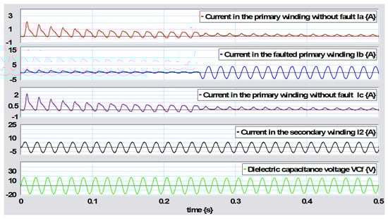
Figure 38.
Transformer behavior under a primary winding turn−to−turn fault.
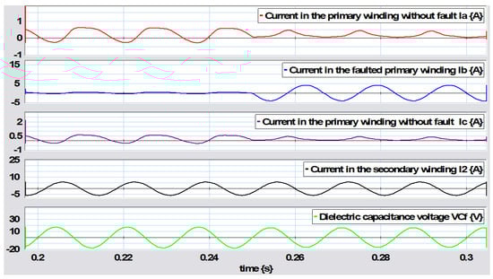
Figure 39.
Inter−turn fault within a short time range.
The steady-state values were obtained by substituting the values given in (116) for a pre-fault condition with , given by
In the failure condition ,
The behavior of the transformer in the case of an inter-turn fault in the primary winding in its steady-state is shown in Figure 40. It can be noted that the current in the section of the primary winding where the fault is located changes, indicating the presence of the fault.
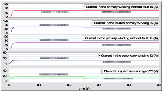
Figure 40.
Steady-state of the inter-turn fault with the BGD.
It is interesting to note that, when a fault occurs, there is no transient at the moment, as the equivalent circuits are the same; only the resistance changes value suddenly with the application of the given fault.
5.4. Arcing Model for Transformer Internal Incipient Faults
In this section, the arcing model for transformers is considered with the aim of showing that the bond graph is a versatile modeling tool. A persistent fault in a transformer would eventually lead to an arc; defined as a continuous luminous discharge of electricity across an insulating medium, usually accompanied by partial volatilization of the electrodes. The model for an arcing phenomenon applied to the transformer on the primary winding is shown in Figure 41.
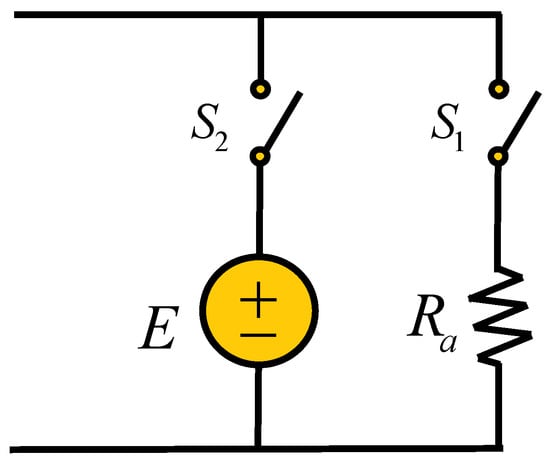
Figure 41.
Arcing model.
The voltage E is a random square wave, and the arc voltage is usually flap-topped. The switches and control the burning and extinction period of an arc, respectively. When arcing is in the burning period, is closed and is open. In the extinction period, is closed and is open. The resistance is a high value.
The bond graph model of the transformer considering the arcing model applied to the primary winding with a fault with respect to the ground is shown in Figure 42.
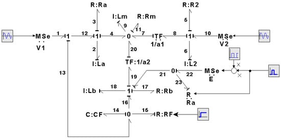
Figure 42.
Arcing model in bond graph.
The bond graph model of Figure 42 is based on the bond graph in Figure 16 corresponding to the fault in the primary winding to ground, adding bonds 21, 22, and 23, which correspond to the voltage source E with a square signal and the resistance . With a voltage V and presenting this fault from 1 s to s and , the behaviors of the transformer variables under both the arcing fault and the traditional primary winding to ground fault are illustrated in Figure 43.
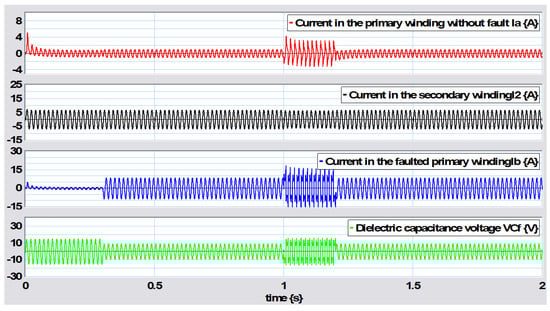
Figure 43.
Primary ground fault and arcing fault.
The primary current waveform is similar to reference [9] and the bond graph model effectively allows the arcing model to be introduced.
5.5. Fault Detection
The objective of this section is to propose a fault detection approach based on a state observer applied to transformers with incipient faults represented using the bond graph approach. Considering the transformer with incipient fault in the primary winding to ground, such a scheme is shown in Figure 44.
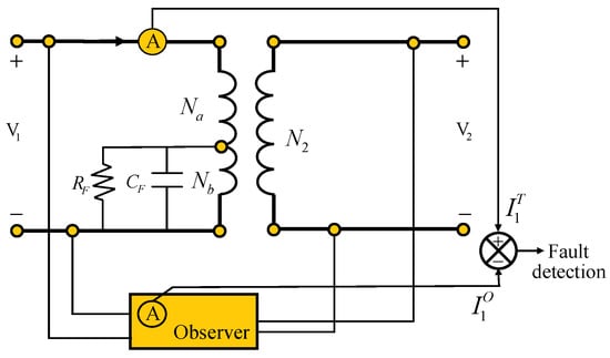
Figure 44.
Transformer observer scheme.
The observer is a circuit design that can consist of analog components or be implemented digitally in such a way that the desired mathematical model is that of the transformer under operating conditions without failure. The observer requires the voltages of the primary and secondary windings and its output is the primary current as the incipient fault is in this winding in this case. The transformer current is monitored and compared with the observer current, allowing a fault to be detected. The associated bond graph model is shown in Figure 45.
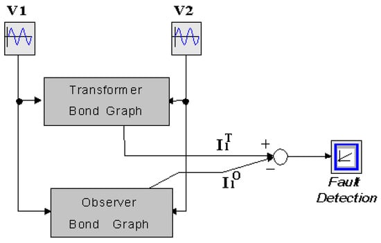
Figure 45.
Bond graph for transformer observer model.
The 20-Sim software allows for the creation of submodels such as those shown in Figure 44 for the transformer observer. However, each submodel is developed as a bond graph. Applying the fault in the primary winding, the results are shown in Figure 46, from which it can be seen that the fault was detected.
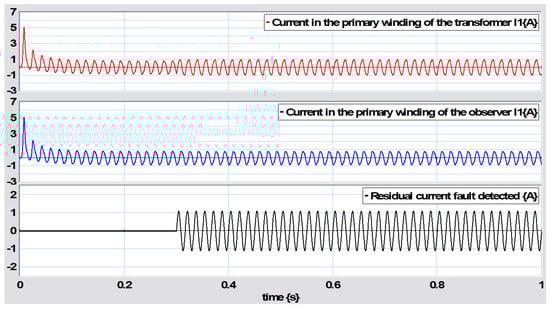
Figure 46.
Transformer, observer, and residual currents.
5.6. Comparison with Other Methods
Numerous works have been published on the modeling, simulation, and detection of incipient faults in transformers. In [3,8,10,13], transformer monitoring systems and the signals monitored for the diagnosis of incipient faults have been described. While mathematical models and simulations were not determined or performed, the locations of sensors for the detection of such faults were indicated. In [4], data from oil-filled transformers were used and a predictive model for incipient failures was proposed. This model was implemented on a computer, and the results were tabulated and compared with known data. In [5], inter-turn faults in transformers were modeled with the inclusion of electromagnetic effects; however, the mathematical model was not described and only this type of fault was analyzed.
Transformer models with incipient faults have been developed using neural networks [6,15], learning systems [12], fuzzy logic [14,16], finite element analysis [17], and intelligent expert systems [18]; however, these works aimed at the computational recognition of faults using such models, and no mathematical models were provided. In [7,9], the simulation of transformers with incipient faults using electrical models was described, and results similar to those obtained via the simulations in this paper were obtained.
To date, real-time fault detection systems have been applied to transformers and other electrical equipment. The magnitudes measured with these systems can be compared with bond graph models in order to test their validity. In these cases, bond graph models using causal paths can indicate which elements will be affected by the propagation of a fault, as well as allowing for consideration regarding whether it is an incipient fault or one due to parametric uncertainty or an external disturbance.
However, there were scarce opportunities to carry out a comparison between this study and those already published. This is mainly because the present study aimed to determine the state-space mathematical model of incipient faults, such that the parameters used were different or not mentioned even in the most relevant references.
6. Conclusions
Models of power transformers with incipient faults developed using a bond graph-based approach were presented in this study. From these graphical models, state-space equations of the transformer models considering magnetic saturation under fault conditions were derived. The links between the bond graphs and the state-space systems were obtained through a junction structure proposed for the considered class of non-linear systems. Likewise, the steady-state response was determined for transformers with various fault conditions and, from the simulation results, it was possible to analyze incipient faults in transformers when applying DC supply sources. The use of the bond graph methodology can be extended to the modeling of transformers, transmission lines, and generators under normal operating conditions as well as under incipient faults in the transformer, thus determining the implications for the rest of the equipment that is part of the system.
Author Contributions
Writing—original draft preparation, A.C.-B.; Writing—review and editing, G.G.-A.; Formal analysis, G.A.-J.; Conceptualization, A.P.G. All authors have read and agreed to the published version of the manuscript.
Funding
This research received no external funding.
Institutional Review Board Statement
Not applicable.
Informed Consent Statement
Not applicable.
Data Availability Statement
The original contributions presented in this study are included in the article. Further inquiries can be directed to the corresponding author.
Conflicts of Interest
The authors declare no conflicts of interest.
References
- Bastard, O.; Bertrand, P.; Meunier, M. A transformer model for winding fault studies. IEEE Trans. Power Del. 1994, 9, 690–699. [Google Scholar] [CrossRef]
- Wang, H.; Butler, K.L. Modeling transformers with internal incipients faults. IEEE Trans. Power Del. 2002, 17, 500–509. [Google Scholar] [CrossRef]
- Morales, E.; Udrescu, R. Active Detection and Identification of Incipient Faults in Liquid Filled Transfomers. In Proceedings of the 2022 IEEE IAS Petroleum and Chemical Industry Technical Conference (PCIC), Denver, CO, USA, 26–29 September 2022. [Google Scholar]
- Igodan, E.; Osajeh, M.; Usiosefe, L. Predictive Model for Incipient Faults in Oil-Filled Transformers. Sak. Univ. J. Comput. Inf. Sci. 2024, 7, 302–313. [Google Scholar] [CrossRef]
- Zhu, N.; Shao, L.; Liu, H.; Ren, L.; Zhu, L. Analysis of Interturn Faults on Transformer Based on Electromagnetic-Mechanical Coupling. Energies 2023, 16, 512. [Google Scholar] [CrossRef]
- Equbal, D.; Khan, S.A.; Islam, T. Transformer incipient fault diagnosis on the basis of energy-weighted DGA using an artificial neural network. Turk. J. Electr. Eng. Comput. Sci. 2018, 26, 77–88. [Google Scholar] [CrossRef]
- Kumar, A.; Rathore, A.; Patra, A. Simulation modeling of incipient faults in power transformer. Int. J. Sci. Eng. Res. 2012, 3, 1–6. [Google Scholar]
- Freire, G.R. Distribution Transformer Incipient Fault Automatic Detection and Monitoring [Extended Abstract]; Instituto Superior Técnico: Lisboa, Portugal, 2020. [Google Scholar]
- Mousavi, M.J.; Butler-Purry, K.L. Transformer internal incipient fault simulations. In Proceedings of the 2003 North American Power Symposium (NAPS), Rolla, MO, USA, 20–21 October 2003; pp. 1–6. [Google Scholar]
- Hu, C.; Zhu, X.; Lu, Y.; Liu, Z.; Wang, Z.; Liu, Z.; Yin, K. Localization and Diagnosis of Short-Circuit Faults in Transformer Windings Injected by Damped Oscillatory Wave. Energies 2024, 17, 6259. [Google Scholar] [CrossRef]
- Ashrafian, A.; Rostami, M.; Gharehpetian, G.B.; Bahnamiri, S.S.S. Improving Transformer Protection by Detecting Internal Incipient Faults. Int. J. Comput. Electr. Eng. 2012, 4, 196–201. [Google Scholar] [CrossRef]
- Saleh, A.M.; Hossain, M.Z.; Rabin, M.J.A.; Kabir, A.M.E.; Khan, M.F.E.; Shahjahan, M. A learning system for detecting transformer internal faults. In Proceedings of the 2013 International Conference on Informatics, Electronics and Vision (ICIEV), Dhaka, Bangladesh, 17–18 May 2013; pp. 1–6. [Google Scholar]
- Goeritno, A.; Nugraha, I.; Rasiman, S.; Johan, A. Injection Current into the Power Transformer as an Internal Fault Phenomena for Measuring the Differential Relay Performance. Instrum. Mes. Metrol. 2020, 19, 443–451. [Google Scholar] [CrossRef]
- Mateus, B.C.; Farinha, J.T.; Mendes, M. Fault Detection and Prediction for Power Transformers Using Fuzzy Logic and Neural Networks. Energies 2024, 17, 296. [Google Scholar] [CrossRef]
- Thango, B.A. On the Application of Artificial Neural Network for Classification of Incipient Faults in Dissolved Gas Analysis of Power Transformers. Mach. Learn. Knowlege Extr. 2022, 4, 839–851. [Google Scholar] [CrossRef]
- Fernandez-Blanco, J.C.; Corrales-Barrios, L.; Bebitez, I.F.; Nuñez-Alvarez, J.R.; Hernandez, F.H.; Losas-Albuerne, Y.L. A proposal for the Diagnosis of Incipient Faults in Power Transformers Using Fuzzy Logic Techniques. Int. Rev. Electr. Eng. 2022, 17, 29. [Google Scholar] [CrossRef]
- Abi, M.; Mirzaie, M. Modelling and Detection of Turn-to-Turn Faults in Transformer Windings Using Finite Element Analysis and Instantaneous Exciting Currents Space Phasor Approach. Int. J. Eng. Manuf. 2014, 5, 12–23. [Google Scholar] [CrossRef][Green Version]
- Hussein, A.R.; Dakhil, A.M.; Rashed, J.R.; Othman, M.F. Intelligent Expert System for Diagnosing Faults and Assessing Quality of Power Transformer Insulation Oil by DGA Method. Misan J. Eng. Sci. 2022, 1, 47–57. [Google Scholar] [CrossRef]
- Ibrahim, A.H.M.; Sadanandan, S.K.; Rajkumar, V.S.T.; Sharma, M. Incipient Fault Detection in Power Distribution Networks, Analysis, Challenges and Future Directions. IEEE Access 2024, 12, 112822–112838. [Google Scholar] [CrossRef]
- Hajiaghasi, S.; Abbaszadeh, K.; Salemnia, A. A New Approach for Transformer Interturn Faults Detection Using Vibration Freequency Analysis. Iran. J. Electr. Electron. Eng. 2019, 1, 14–28. [Google Scholar]
- Sharma, P.; Patel, R.A. Modelling and Simulation of Condition Monitoring of Three Phase Transformers using Matlab. J. Emerg. Technol. Innov. Res. 2021, 8, 1068–1075. [Google Scholar]
- Namdari, F.; Bakhshipour, M.; Rezaeealam, B.; Sedaghat, M. Modeling of Magnetizing Inrush and Internal Faults for Three-Phase Transformers. Int. J. Adv. Appl. Sci. 2017, 6, 203–212. [Google Scholar] [CrossRef][Green Version]
- Odongo, G.; Musabe, R.; Hanyurwimfura, D. A Multinomial DGA Classifier for Incipient Fault Detection in Oil-Impregnated Power Transformers. Algorithms 2021, 14, 128. [Google Scholar] [CrossRef]
- Ashrafian, A.; Naderi, M.S.; Gharehpetian, G.B. Detection of internal incipient faults in transformers during impulse test using hyperbolic S-transform. Int. Trans. Electr. Energy Syst. 2013, 23, 701–718. [Google Scholar] [CrossRef]
- Sueur, C.; Dauphin-Tanguy, G. Bond graph approach for structural analysis of MIMO linear systems. J. Frankl. Inst. 1991, 328, 55–70. [Google Scholar] [CrossRef]
- Sueur, C.; Dauphin-Tanguy, G. Bond graph approach to milti-scale systems analysis. J. Frankl. Inst. 1991, 328, 1005–1026. [Google Scholar] [CrossRef]
- Gonzalez, G.; Ayala, G.; Barrera, N.; Padilla, A. Linearization of a Class of Nonlinear Systems Modelled by Multibond Graphs. Math. Comput. Model. Dyn. Syst. 2019, 25, 284–332. [Google Scholar] [CrossRef]
- Controllab Products. Available online: www.20sim.com (accessed on 3 June 2025).
- Karnopp, D.C.; Margolis, D.L.; Rosenberg, R.C. System Dynamics: Modeling, Simulation, and Control of Mechatronic Systems; John Wiley & Sons, Inc.: Hoboken, NJ, USA, 2012. [Google Scholar]
- Thoma, J.; Bouamama, B.O. Modelling and Simulation in Thermal and Chemical Engineering: A Bond Graph Approach; Springer: Berlin/Heidelberg, Germany, 2000. [Google Scholar]
- Dauphin-Tanguy, G. Les Bond Graphs; Hermes: Paris, France, 2001. [Google Scholar]
- Amirdehi, S.; Trajin, B.; Vidal, P.E.; Vally, J.; Colin, D. Power transformer model in railway applications based on bond graph and parameter identification. IEEE Trans. Transp. Electrif. 2020, 6, 774–783. [Google Scholar] [CrossRef]
- Fujiwara, E. Multidomain Systems Modeling with SPICE: Equivalent Circuit and Bond Graph Approaches. IEEE Rev. Iberoam. Tecnol. Del Aprendiz. 2025, 20, 39–46. [Google Scholar] [CrossRef]
- Guo, Z.; Korondi, P.; Szemes, P.T. Bond-Graph-Based Approach to Teach PID and Sliding Mode Control in Mechatronics. Machines 2023, 11, 959. [Google Scholar] [CrossRef]
- Puras, B.; Raush, G.; Freire, J.; Filippini, G.; Roquet, P.; Tirado, M.; Casadesus, O.; Codina, E. Development of a Virtual Telehandler Model Using a Bond Graph. Machines 2024, 12, 878. [Google Scholar] [CrossRef]
- He, F.; Hang, J.; Yu, W.; Zhong, G. Fault Diagnosis of the Three-phase Asynchronous Motor Bond Graph Model Based on Bond Graph and Temporal Causal Graph. J. Phys. Conf. Ser. 2023, 2428, 012017. [Google Scholar] [CrossRef]
- Liu, N.; Li, C.; Zhang, L.; Lei, Z.; Yang, J.; Lai, F. The Bond Graph Modeling and Experimental Verification of a Hydraulic Inertial Vibration Isolator Including Nonlinear Effects. Aerospace 2024, 11, 634. [Google Scholar] [CrossRef]
- Sellami, A.; Aymen, Z.M.; Feki, E.; Mami, A. Reliability of the Bond Graph Approach for Robust Diagnosis of a Newborn Incubator System. Lond. J. Eng. Res. 2024, 24, 47–72. [Google Scholar]
- Gawthrop, P.J.; Pan, M. Energy-based Analysis of Biochemical Oscillators Using Bond Graphs and Linear Control Theory. bioRxiv 2024. [Google Scholar] [CrossRef] [PubMed]
- Wootton, M.J.; Andrews, J.D.; Smith, R.; Arul, A.J.; Vinod, G.; Prasad, M.H.; Garg, V. An integrated Petri net-pseudo bond graph model for nuclear hazard assessment. Saf. Reliab. 2024, 43, 135–185. [Google Scholar] [CrossRef]
- Ghazani, M.A.; Pan, M.; Tran, K.; Rampadarath, A.; Nickerson, D.P. A review of the diverse applications of bond graphs in biology and physiology. Proc. R. Soc. A 2024, 480, 20230807. [Google Scholar] [CrossRef]
- Gonzalez, G.; Galindo, R. Steady state determination using bond graphs for systems with singular state matrix. Proc. Inst. Mech. Eng. Part I J. Syst. Control Eng. 2011, 225, 887–901. [Google Scholar] [CrossRef]
- Krause, P.C.; Wasynczuk, O.; Sudhoff, S.D. Analysis of Electrical Machinery and Drive Systems; Wiley-IEEE Press: Hoboken, NJ, USA, 2002. [Google Scholar]
- Garcia, S.; Medina, A.; Perez, C. A state space single-phase transformer model incorporating nonlinear phenomena of magnetic saturation and hysteresis for transient and period steady-state analysis. IEEE Power Eng. Soc. Summer Meet. 2000, 4, 2417–2421. [Google Scholar]


Disclaimer/Publisher’s Note: The statements, opinions and data contained in all publications are solely those of the individual author(s) and contributor(s) and not of MDPI and/or the editor(s). MDPI and/or the editor(s) disclaim responsibility for any injury to people or property resulting from any ideas, methods, instructions or products referred to in the content. |
© 2025 by the authors. Licensee MDPI, Basel, Switzerland. This article is an open access article distributed under the terms and conditions of the Creative Commons Attribution (CC BY) license (https://creativecommons.org/licenses/by/4.0/).