Abstract
To solve the problem of high cost and low efficiency of measuring equipment in traditional distribution network fault location, a fault section location and line selection strategy combining dynamic binary particle swarm optimization (DBPSO) configuration and fuzzy C-means (FCM) clustering is proposed in this paper. Firstly, the DBPSO algorithm is used to optimize the configuration scheme of the distributed voltage and current sensing device, which reduces the number of measuring devices and system cost on the premise of ensuring the global observability of the distribution network. When a fault occurs in the distribution network, the sensor device based on optimal configuration collects fault feature data, combines it with the FCM clustering algorithm to classify nodes according to fault feature similarity, and divides the most significant fault-affected section as the core fault area. Further, by calculating the Euclidean distance between each node in the fault section and the cluster center, the fault line is accurately identified. Finally, a fault simulation model based on an IEEE 11-node system is constructed to verify the effectiveness of the proposed method. The results show that, compared with the traditional fault section location and route selection strategy, this method can reduce the number of measurement devices optimally configured by 19–36% and significantly reduce the number of algorithm iterations. In addition, it can realize rapid fault location and precise line screening at a low equipment cost under multiple fault types and different fault locations, which significantly improves fault location accuracy while reducing economic investment.
1. Introduction
When the distribution network fails, in order to prevent further expansion of the fault area, reduce economic losses, and improve the reliability of power supply, fast and accurate fault location is very necessary.
China’s distribution network is mostly low and medium voltage overhead lines, and is located in a complex environment [1], many branch circuits, susceptible to a variety of factors and blackout accidents, the data show that the distribution network faults caused by blackouts accounted for the probability of user blackouts as high as 96% of the accident, which makes the national economic losses are more serious. In order to ensure the operation of the distribution network, make it safe and reliable, we can start from two aspects. On the one hand, the purpose is to reduce the number of failures, in this regard, we in addition to the strict implementation of the safe operation of distribution network lines, reduce human damage, such as lightning, lightning and other irresistible factors are beyond our control, so it is difficult to reduce the occurrence of failures from the source. Therefore, our focus will be on the other side (i.e., fast, accurate, and low-cost localization of faults). When a fault occurs in the distribution network, we can quickly and accurately determine the location of the fault, isolate the faulty area, avoid the expansion of the scope of the power outage, shorten the time of manual troubleshooting by the staff, and quickly restore the power supply to minimize the economic losses. Therefore, it is of practical and economic significance to carry out fast and accurate, low-cost fault localization in distribution networks [2,3,4,5,6,7].
The methods for locating faults vary according to different standards. There are not only some new power grid protection equipment used to help locate the fault location, such as solid state circuit breakers [8,9], but also many intelligent location methods that realize multi-criterion fusion by comprehensive mathematical analysis. In this paper, the impedance method, the transient analysis method, the traveling wave method, and the integrated location method are introduced in detail.
The impedance method is affected by line impedance, multiple branches, load, transformer characteristics, and pseudo-fault points. Reference [10] conducts the first preliminary positioning based on the impedance legal level and then combines the specific network topology to propose a coefficient correction method for secondary positioning, thereby solving the problem of branch load. This method improves the accuracy and feasibility of impedance at the legal level. However, the location results are greatly affected by the fault distance and transition resistance, and the application range is small.
Although the transient reactive power direction method and the transient zero mode current method have advantages, the location result of the former is affected by fault distance and transition resistance, and the latter needs further practice to improve its adaptability. Reference [11] combines transient zero-mode current with maximum RMS, inner product, and correlation theory to conduct fault line selection, and compares the correlation coefficient of transient zero-mode current at adjacent detection points with the threshold value to achieve fault location. This method has high accuracy and reliability, but further practical research is needed to improve its adaptability in actual operation.
The traveling wave method is difficult to operate in a distribution network because of the many branches and the weak reflection signal of the traveling wave. The calculation of the single-ended traveling wave method is complicated, and the synchronization and economy problems need to be solved by the double-ended traveling wave method. The single-ended traveling wave method in reference [12] combines the fault point and the opposite bus to reflect the swept voltage and the electric popular wave signal to improve the ranging accuracy and reliability. Although it is suitable for a single-phase grounding fault, the calculation is complicated. Two-end traveling wave ranging is located according to the absolute time from the traveling wave to both ends of the line, and the synchronization of both ends should be considered. Reference [13] proposes a new method based on the midpoint of time, which is not affected by the medium and can be used in the case of multiple media, but it needs to keep the measurement of electrical volume synchronized and has low economy. It is difficult to use the traveling wave method to locate faults in a distribution network. It is difficult to distinguish traveling waves caused by multiple branches of the distribution network, and the traveling wave reflection weakens the signal and affects the location accuracy.
In this paper, the optimized configuration of BPSO with distributed voltage and current sensing devices and fuzzy C-means algorithm is used to realize fault zone localization. The optimized configuration of distributed voltage and current sensing devices in a distribution network, achieved by a dynamic binary particle swarm algorithm, reduces the number of measuring devices equipped and the cost of fault location under the condition of realizing the viewability of the whole distribution network. Then according to the voltage and current of each bus node, the positive sequence voltage, zero sequence current, and zero sequence impedance angle of each node at the time of fault are used as the feature vectors of the algorithm, and the bus nodes of the distribution network are classified into three categories, where the faulty nodes form the faulty region, and then the faulty lines are determined by calculating the Euclidean distance between each node in the faulty region and each category. Finally, MATLAB is utilized for simulation and programming to verify the region localization and line selection under various fault states, and take the single-phase grounding fault of the IEEE14 node as an example.
2. Optimized Configuration of DBPSO-Based Distributed Voltage and Current Sensing Devices
A distributed voltage and current sensing device is a new data measurement device developed to solve the bottleneck of data collection in the distribution network. By configuring the device on the power system bus, the real-time data of voltage, current, and power on the line can be obtained at the IoT communication unit. When a fault occurs, the fault recording waveform can be obtained and uploaded and output through the IoT communication unit, and the storage group can be carried out. This chapter describes a distributed voltage and current sensing device based on the dynamic binary particle swarm algorithm for the optimal configuration of the distribution network, to reduce the number of measuring devices equipped, and to reduce the cost of fault localization under the condition of realizing the observability of the whole distribution network.
2.1. Distribution Network Observability
Observability of the distribution network refers to the calculation and estimation of the current operating state of the system based on the quantity measurement and distribution of the current system, also known as the observability of the distribution network. Observability analysis of the distribution network is an important part of its state estimation, and it is also one of the preconditions for fault location.
Distributed voltage and current sensing device can easily measure voltage, current, power and other data information, if each node in the distribution network is configured with the device, all the real-time data of the distribution network can be obtained, and the operating state of the current system can be judged through these data without any calculation to achieve complete visibility of the distribution network. However, considering the efficiency problem and further cost reduction, it is necessary to optimize the configuration of the device to ensure complete observability, high efficiency, and economy of the distribution network, and to realize the full utilization of the measured data of the measuring device. When the sensor device is optimally configured, the state quantity of some nodes can be directly measured. The state quantity of such nodes includes the voltage vector of the bus node where the sensor device is installed and the current vector of the branch connected to the node, while the electrical quantity of the remaining nodes is unknown. To optimize the configuration of distributed voltage and current sensing devices to achieve the observability of the distribution network, it is necessary to obtain the electricity volume of nodes that cannot be measured on the basis of part of the measurement information measured by the device, so as to meet the observability requirements of distribution network.
For a bus node installed with a distributed voltage and current sensing device, the real-time data of the voltage vector and the current vector of the branches connected to it and the changing waveform can be directly output by the iot communication unit. In contrast, the voltage vector of the bus node without a measuring device can be indirectly obtained by Kirchhoff’s current law (KCL) and Ohm’s law. If the voltage phasors of all bus nodes can be measured directly or calculated indirectly, then the observability of the power system can be satisfied. For nodes that need indirect calculation, it can be summarized into two aspects:
(1) The voltage vector of the bus node equipped with a distributed voltage and current sensing device and the current phasor of the connected branch are known, and the voltage vector of another node that can be connected to the branch is calculated;
(2) If a node is connected to b branches, if the current vector of b − 1 branches is known, the current vector of the b branch can be obtained by KCL.
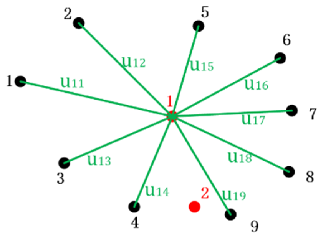
As shown in Figure 1, nodes 1 and 2 are equipped with distributed voltage and current sensing devices to analyze the observability of nodes 3 and 4.
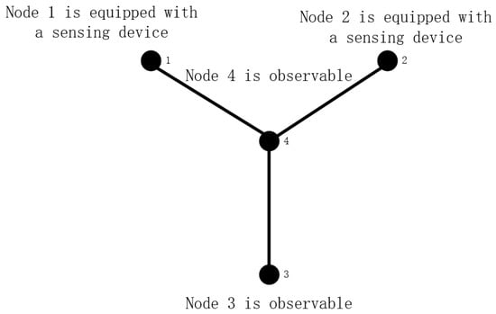
Figure 1.
Observability analysis of distribution grids.
Node 1 and node 2 are observable points; that is, U1, U2, I14, and I24 are known quantities. According to Article (1) of indirect calculation induction, U4 can be obtained, that is, node 4 is observable. According to Article (2) of indirect calculation and induction, I34 can be obtained, under the condition of obtaining U4 and I34, and then summarized by Article (1), U3 can be obtained, and node 3 is also an observable node, so the power distribution system has observability. For a power distribution system to be observable, one of the following conditions must be met:
(1) The node is equipped with a distributed voltage and current sensing device, so that the voltage phasor and the current phasor of adjacent branches can be measured, and the node meets the observability criteria.
(2) This node is not equipped with a distributed voltage and current sensing device. If the voltage phasor of this node and the current phasor of adjacent branches can be calculated indirectly because other nodes are equipped with sensing devices, then this node is also observable.
In order to effectively evaluate and compare the DBPSO results, we decided to introduce the lower bound of device configuration based on Kirchhoff’s law. In the distribution network, the voltage vector of the bus node without the measurement device can be indirectly obtained by KCL and Ohm’s law. When the voltage phasors of all bus nodes can be directly measured or indirectly calculated, the power system satisfies observability. For the nodes that need indirect calculation, it is mainly summarized into two aspects: on the one hand, when the voltage vector of the bus node equipped with distributed voltage and current sensing devices and the current phasor of the connected branch are known, the voltage vector of the other node connected to the branch can be calculated; on the other hand, if a node is connected to b branches, when the current vector of b−1 branches is known, the current vector of b branches can be obtained by KCL. Based on this, we determine that the lower bound of the device configuration is N − 1 (where N is the total number of nodes). In this way, we can provide a comparative benchmark for the DBPSO results to evaluate their performance more accurately.
2.2. Iterative Optimization Method
There are many optimal configuration methods of measuring devices at home and abroad [14,15,16,17,18], such as numerical optimization algorithms and heuristic optimization algorithms. The numerical optimization algorithm can be divided into the exhaustive method and the integer programming method. The exhaustive method is generally applied to unit coherency analysis and can only be applied to simple, small systems, which is not ideal for complex, large systems. The integer programming method generally simplifies the constraint conditions and logics of the complex problems, so as to expand the scope of application. However, sometimes the obtained model is nonlinear, the solution is very difficult, and the operational efficiency is not high, which has certain limitations. Heuristic optimization algorithms include many intelligent optimization algorithms. Compared with numerical algorithms, intelligent optimization algorithms have a wider range of applications and stronger global search capabilities, showing great superiority in solving optimization problems. In addition, there are algorithms based on the system topology model, such as the minimum spanning tree algorithm. The intelligent optimization algorithm has strong model adaptability and global searching ability, so it is widely used. The main idea is to obtain the optimal solution by establishing the objective function to iterate, and to observe whether the difference between the objective function values before and after the iteration meets the judgment conditions of the algorithm until the maximum number of iterations of the algorithm.
2.3. Allocation Optimization Algorithm
A DBPSO algorithm based on fixed inertia weight and increasing constraints is used to optimize the configuration of distributed voltage and current sensing devices in a distribution network. Since the search space of the optimal configuration problem of this device belongs to the discrete binary space, the particle swarm optimization algorithm is no longer applicable, and the binary particle swarm optimization algorithm is needed to solve the problem. In the binary particle swarm optimization algorithm, the selection of the inertia weight will have a certain impact on the optimization process. Therefore, the fixed inertia weight is selected by comparison to adjust its global search ability, reduce the number of iterations, and reduce the number of times that it falls into the local optimal solution. When optimizing the configuration, the correlation degree between the bus nodes of the distribution network is considered, and more system information can be obtained when the system is closely related.
2.3.1. Particle Swarm Algorithm
The particle swarm optimization (PSO) algorithm is used to find the optimal solution by iteration from a random solution. Individually, each particle endeavors to identify the most favorable outcome within its search domain, marking this as its present personal best. This personal best is then communicated to the rest of the swarm members. The collective aim is to pinpoint the most superior personal best, which is regarded as the swarm’s current best overall solution. Guided by their discovered personal bests and the swarm’s shared best solution, each particle modifies its velocity and position accordingly within the swarm. During the whole search process, the velocity vector v and the position vector x of the individual, i.e., the particle, are constantly updated and changed, as shown in Equations (1) and (2).
In the formula, c1 and c2 represent the weight coefficients of the particle tracking itself and the historical optimal value of the tracking group, respectively; Random numbers uniformly distributed in r1 and r2 interval [0, 1]; v and x represent the velocity vector and position vector, respectively; d and k represent the spatial dimension and the number of iterations, respectively; pbestk represents the optimal position of the particle i in the d dimension until the k-th iteration; gbestk represents the optimal position of all particles in the solution process during the k-th iteration; w represents inertia weight.
In the search process, there are two bases for the change of the position vector and the velocity vector. One is the influence of the position of the most likely optimal solution in the search process, and the other is the influence of the position of the global optimal solution.
Typically, the stopping criterion for an iteration is set to either reach the highest iteration count set for the particle swarm optimization or to find an optimal solution that falls within a pre-established minimum threshold tailored to the particular problem at hand. Increasing the iteration cap for the PSO process tends to enhance the precision of the outcome. Typically, this cap is set higher than the iterations needed for a particle to find the best solution, ensuring that the algorithm concludes once this higher iteration limit is met.
2.3.2. Binary Particle Swarm Optimization
The biggest difference between the BPSO algorithm and the PSO algorithm is the solution space. The former mainly solves the combinatorial optimization problem in the discrete space, and the latter’s solution space is continuous. In BPSO, the historical optimum and global optimum of each dimension of the particle and the particle itself are limited to 1 or 0, and the velocity is not limited. The velocity vector is updated by comparing the set threshold with the velocity. When the velocity is higher than the threshold, the position of the particle is 1; otherwise, it is 0.
Different from the speed formula of the PSO algorithm, the speed value of the BPSO algorithm will be mapped to the [0, 1] interval by the sigmoid function into the probability of the variable taking 1, as shown in the Equation (4), which is the probability that the particle takes 1 in the next step.
rand () represents the number randomly generated in the uniform distribution of the interval [0, 1]; s(vid) represents the probability that the particle trajectory is currently 0.
s(vid) only represents the probability that the particle takes 1 in the next step, but does not represent the probability that the particle position changes. It can be seen from Equation (4) that the smaller the particle velocity vid is, the closer the probability function sigmoid is to 1, that is, the greater the probability that the particle position is updated to 1, and vice versa, the closer sigmoid is to 0. Because the optimal configuration problem of the distributed voltage and current sensing device in the distribution network is solved in the discrete space, the BPSO algorithm is selected.
2.3.3. Fitness Function
The algorithm used in this paper considers the node correlation degree under the condition that the distribution network is completely observable, thereby increasing the constraints. Considering the influence of inertia weight on the performance of the algorithm, the appropriate weight is selected to reduce the number of distributed voltage and current sensing devices, reduce the number of iterations, and the expression of fitness function and constraints is as follows.
N is the total number of nodes; ki represents the configuration of the measurement device on the node, with 1 for the equipped device and 0 for the other; Arel represents an N × N node incidence matrix; K represents the set of configurations of the node device in the system.
According to the fitness function, ki represents the device configuration of node i. If the node i is equipped with the device, then the aijki value is 1, which satisfies the constraint condition Equation (7); if the node i is connected to the node j, and the node j is equipped with a distributed voltage and current sensing device, then the value of aijkj is 1, that is, the voltage phasor of the node i can be calculated by the node j, which satisfies the observability of the node i and satisfies the constraint condition Equation (7). If the node i and the node connected to the node j are not equipped with a distributed voltage and current sensing device, then the constraint condition 7 is not satisfied, that is, mi = 0, and the constraint condition ensures the observability of the distribution network.
In the new constraint condition Equation (8), b is a constant, indicating that when the number of nodes connected to node i exceeds b, the distributed voltage and current sensing device is installed at the node. The size of b can change with the complexity of the topological structure. When the node system is relatively simple, b can take a smaller value. When the node system is more complex and the nodes are more closely connected, the value of b can be appropriately increased. It makes the data obtained by the measuring device more sufficient and reliable, the positioning result more accurate, and the measurement range larger.
2.3.4. Selection of Inertia Weight in Fitness Function
Inertia weights are chosen to balance the global and local search capabilities of binary particle swarm optimization. At the early stage of iteration, the larger inertia weight helps the global particle exploration and reduces the probability of falling into a local optimum. In the later stage, the weight is reduced, the communication between particles is strengthened, and the local search is focused on improving the precision of the solution.
The selection of the inertia weight has a great influence on the operation result and operation efficiency, so it is of great practical significance to improve the inertia weight of the algorithm. On the basis of selecting the appropriate inertia weight, the distributed voltage and current sensing device is optimized according to the algorithm. The optimal configuration of the IEEE9 node model is analyzed in detail, and several standard node systems are verified.
Inertia weight is an important parameter. Its selection has a certain influence on the optimization results and the number of iterations. By comparing the operation results of IEEE39 nodes and IEEE123 nodes under different weight selections, the appropriate inertia weight is selected for the optimal configuration of the distributed voltage and current sensing device in the distribution network.
Inertia weights in particle swarm optimization can be categorized into two types: static and dynamic. The static inertia weight involves assigning a constant value, which remains consistent throughout the optimization, thereby endowing particles with a consistent level of exploration and exploitation abilities. Conversely, the dynamic inertia weight is adjusted in accordance with a predefined pattern over a specified range during iterations, granting particles varying degrees of exploration and exploitation abilities at different stages of optimization. Different inertia weights have different effects on the operation results of the algorithm. The fixed weight [19,20] is compared with other time-varying weights. The comparison results show that the fixed weight is more suitable for the optimal allocation of distributed voltage and current sensing devices in the distribution network than the time-varying weight. The inertia weight selection scheme is shown in Table 1, and the time-varying weight change rule is shown in Table 2.

Table 1.
Selection of fixed inertia weight.
Table 2.
The change law of time-varying weight.
In the selection scheme, schemes 1 and 2 are fixed-weight selection schemes, and schemes 3, 4, and 5 are time-varying weight selection schemes. Among them, wmin is the minimum inertia weight value, and wmax is the maximum inertia weight value. In the weight change rule, t is the current iteration number, Tmax is the maximum iteration number, which is set to 1000, and the particle swarm size is set to 20. The comparison results of scheme 1 are shown in Table 3, and the comparison results of schemes 3, 4, and 5 under different weight variation rules are shown in Table 4, Table 5 and Table 6, respectively.
Table 3.
Comparison result of the inertial weighting scheme 1.
Table 4.
Comparison result of the inertial weighting scheme 3.
Table 5.
Comparison result of the inertial weighting scheme 4.
Table 6.
Comparison result of the inertial weighting scheme 5.
When the number of nodes is relatively small, the results of all inertia weight selection schemes are not much different when comparing the number of devices configured and the number of iterations. But as the number of nodes increases, the fixed weight has obvious advantages over other selection schemes. Running with fixed weights, the number of configurations for the distributed voltage and current sensing device is relatively small, and the number of iterations required is far less than that of other schemes. Therefore, considering comprehensively, the fixed weight is selected as the inertia weight of the fitness function, that is, w = 0.729, c1 = c2 = 1.494.
2.3.5. Dynamic Sensors Optimize Time Segmentation
Compared with the traditional binary particle swarm optimization algorithm, the dynamic particle swarm optimization algorithm can be used for the sensor configuration optimization of distribution networks with load changes. This algorithm can make good use of the detection mechanism and the corresponding mechanism to lock the fitness function. For the changing functions in the distribution network, it can quickly change the positions and velocities of sensitive particles in the population to adapt to the dynamic environment.
Taking into account the load variation of the distribution network, the time can be segmented as follows:
(1) According to the results of regional load forecasting of the distribution network, the future change of regional load can be predicted.
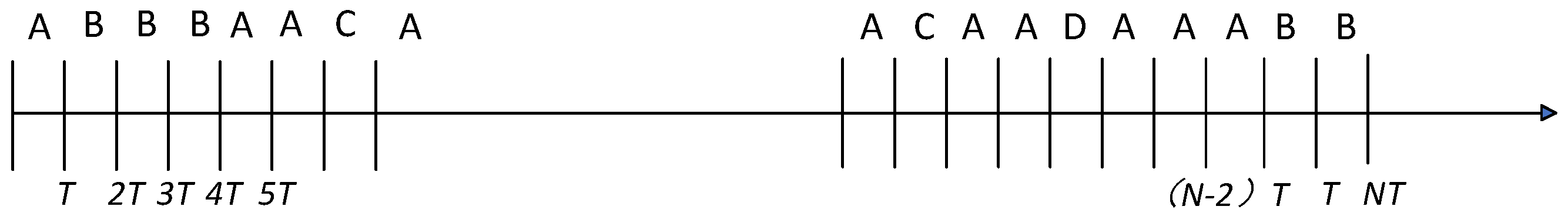
(2) At a certain time interval T, according to load prediction data f(nT) of the corresponding time section, an artificial intelligence algorithm is used to optimize the configuration of distribution network sensors. After a series of optimizations, the results are obtained as shown in Figure 2, where A, B, C, and D are four operating modes.
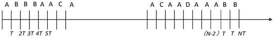
Figure 2.
Segmented optimization result.
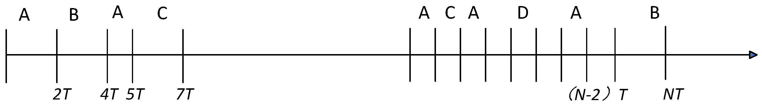
(3) In the optimization result of the previous step, time periods with the same optimization scheme can be merged, as shown in Figure 3.
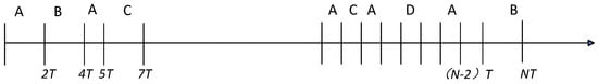
Figure 3.
With the results of the optimization method.
(4) According to the optimization results of the previous step, if there are definitely different optimization modes in adjacent time periods, for example, optimization mode A is better for segment [0, T], and optimization mode B is better for segment [2T, 4T], it is necessary to determine whether it is necessary to switch all these modes in this step. Then define two adjacent time periods as M and M + 1, make the sequence number of the first time period as 1 and the sequence number of the last time period as N, and then calculate the evaluation function g(XM, XM) and g(XM, XM+1). They represent the profit and loss of adopting XM mode in the M and M + 1 time periods and switching from XM to XM+1 mode at the junction, respectively. The expression is:
where: AXM [f(t)] and AXM+1 [f(t)] are the index calculation functions of XM and XM+1, and active power loss can be used here.
(5) WS is defined as the minimum income threshold of mode switching, and compared with the difference of the above indicator functions, mode switching is required only when the income value after the current mode switching exceeds WS; otherwise, mode switching is not necessary to avoid the operational risks and costs caused by too frequent switching.
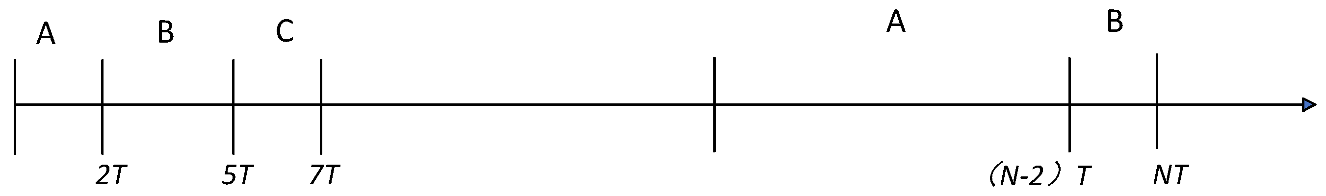
(6) As shown in Figure 3, mode A is used in (0, 2T) and mode B is used in (2T, 4T). If the mode switching between (2T, 4T) and (4T, 5T) is less than the minimum return threshold, the two periods can be combined without switching from mode A to mode B. Similarly, the final optimization result is shown in Figure 4.

Figure 4.
Dynamic optimization of the final result.
Using the above method, according to the results of load prediction, optimize the operation mode and switching time in the future period, and determine whether it is necessary to switch and avoid unnecessary operations by giving the function of the minimum income threshold.
2.3.6. Distribution Network Sensor Optimization for Load Variation
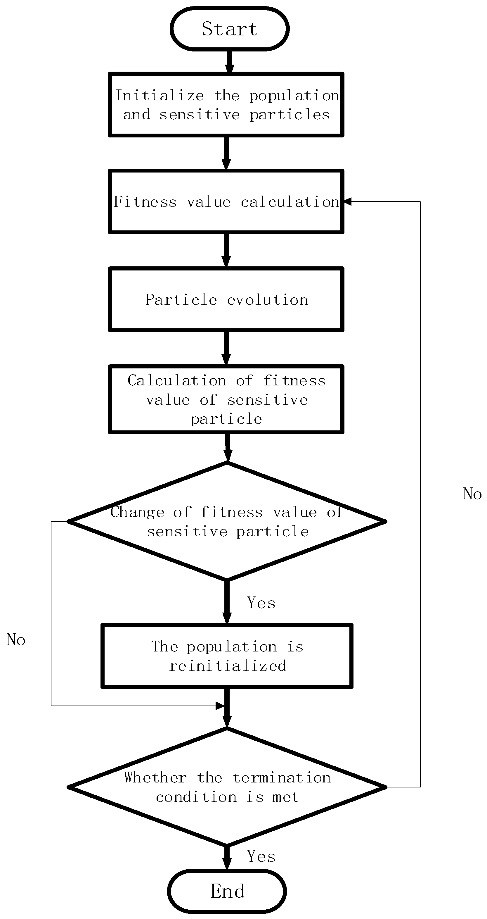
In view of the load in the distribution network changing with time, the conventional binary particle swarm optimization algorithm is improved. First, the detection mechanism is introduced to enable the population or particle to perceive changes in the external environment. The second is to introduce a response mechanism. After detecting the change in the environment, the population is updated in a response way to adapt to the dynamic environment. Mainly, when the load in the distribution network changes, the speed and position of the newly updated particles are updated through intelligent detection and identification of the change of parameters in the distribution network, and a better fitness value is obtained. The main process is shown in Figure 5.
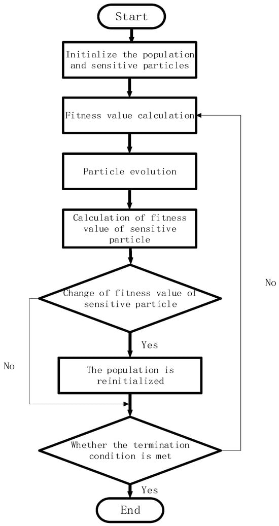
Figure 5.
Dynamic binary particle swarm algorithm flow.
The optimization steps of the distribution network sensors based on dynamic particle swarm optimization are as follows:
(1) Initialize the data of the distribution network system, and determine the division of the time period according to the load prediction results, so that the total time is h, and the time period is divided into n segments. Record the status of the normally open switch and the normally closed switch in the system, and record the status of the normally open switch as 1, and the status of the off switch as 0.
(2) The dynamic particle swarm optimization algorithm is initialized, active power loss is used as the calculation of fitness value, the lowest fitness value is obtained through the corresponding number of iterations, the action scheme of the corresponding switch is given, and the time segment is 1.
(3) When entering the time segment 2, part of the load in the power distribution system changes to a certain extent due to changes in demand. At this time, the particles evolve according to the detection of the dynamic particle swarm and the corresponding mechanism, and the fitness value is adjusted by changing the position and speed of the particles. The lowest fitness value is calculated iteratively, and the secondary optimization is carried out to obtain a new configuration mode. In this case, you need to make a decision to determine whether the switching revenue of the two modes exceeds the minimum threshold. If the switching revenue does not exceed the minimum threshold, you do not need to switch the modes. If the switching revenue exceeds the minimum threshold, you need to switch the modes to achieve the best operating mode of the system.
(4) The dynamic distribution network sensor optimization is carried out according to the time segment. Each time, the particle population needs to be re-initialized, but at the same time, the new optimal solution can be reached only with a small number of iterations. When the time reaches the last period, different operation modes are sorted out, that is, the best operation mode for a certain period or several periods.
3. Fault Section Location and Line Selection Algorithm
The clustering analysis method needs to be based on the similarity or distance of sample features as the basis for determining whether a sample belongs to a certain category. In cluster analysis, there are many ways to measure the similarity of sample features, such as Minkowski distance, Mahalanobis distance, correlation coefficient, cosine angle, and so on. The fuzzy C-Means algorithm is a clustering algorithm based on the objective function. Different from the classic clustering algorithms, it has uncertainty in the division of the analysis object. This uncertainty is manifested in the space of the mapping of the set to be found. The set to be found X maps the fuzzy result onto the space [0, 1]. This mapping result is not a probability but represents a degree of similarity, that is, the membership degree of the sample, which is used to represent the degree of similarity that a sample belongs to the result. It is an indicator of the degree to which a sample is similar to different results. Finally, Euclidean distance is chosen as the distance measurement of the FCM algorithm because Euclidean distance represents the real distance between two feature quantities, which is relatively simple and intuitive in practical applications. Other distance measurement methods have some shortcomings, such as Minkowski distance, which treats all components equally and does not consider the difference between different features and the dimensional influence. Mahalanobis distance has the problem of exaggerating small variables. The correlation coefficient is applicable only when the feature dimension is large enough, and it is greatly affected by the k value. In contrast, Euclidean distance is more suitable for measuring the similarity between samples in the FCM algorithm to achieve accurate clustering and fault location.
When a short-circuit fault occurs, the fault characteristics of each node will change to varying degrees. The distance between each node and the fault location is different. According to this feature, combined with multiple fault characteristics, the FCM in the cluster analysis method is used to locate the fault section of the distribution network. On this basis, the fault line is judged by comparing the Euclidean distance between each node and each category in the fault section.
3.1. Fuzzy C-Means Algorithm
Spatial fuzzy C-means algorithm [21,22,23,24] is a fuzzy clustering algorithm based on the objective function. Different from the classical clustering algorithm [25], it has uncertainty in the division of the analysis object. This uncertainty is manifested in the space of the mapping of the set to be sought. The set to be sought X maps the fuzzy results to [0, 1]. The mapping result is not a probability, but represents a degree of similarity, that is, the membership degree of the sample. It is used to indicate the similarity of a sample to the result. It is a degree index that a sample is similar to different results.
In this paper, the object to be analyzed by the FCM algorithm is each node, and the feature vector of each node is composed of multiple fault feature components. If the set to be analyzed is X, then X = {x1, x2, … xn} is the feature vector set of multiple nodes to be classified, and then xi = {xi1, xi2, … xiq} represents each feature of each node. If the FCM method is used to divide these objects to be analyzed into c classes (c ≥ 2), each class has a corresponding class center C, and the class center vector can be expressed as C = {c1, c2, … ck}, where ck is the corresponding class center of each class, so that the membership degree of each sample xi belonging to a certain class of k is uki. The objective function and its constraint conditions of the FCM method are shown in Formulas (11) and (12).
In the formula, m-membership factor;
The goal-oriented function is constructed by taking the degree of membership of each instance and combining it with the measure of how far that instance is from the centroid of its respective category, m can be understood as the degree of ease of belonging to the sample; the constraint condition requires the sum of the membership degree of a sample belonging to all classes to be 1. It is a continuous iterative process to obtain the objective function by using the FCM method, that is, the membership degree uki and the class center ck are not fixed quantities, and their iteration formulas are as follows.
The iteration of the membership degree and class center is very important to the operation of the algorithm. The two are interrelated and contain each other. Therefore, at the beginning of the iteration, generally give uki an initial value that meets the constraints, and then iterate. In the iterative process, the objective function gradually tends to a stable value. The relationship between the two is shown in Figure 6 and Figure 7.
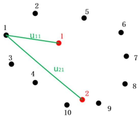
Figure 6.
Macroscopic membership analysis chart.

Figure 7.
Macroscopic class center analysis chart.
Black represents the sample, red represents the class center, and green represents the membership relationship between the sample and the class center, as shown in Equations (15) and (16).
Figure 6 observes the iterative formula of membership degree from a macro perspective, which represents the membership degree from sample 1 to each class center. The ratio of the distance from sample 1 to a class center to the sum of the distances from sample 1 to each class center is the similarity between the sample and the class center. The larger the corresponding uki is, the closer the sample is to this class.
Black represents the sample, red represents the class center, and green represents the relationship between the class center and the sample, as shown in Formula (17).
Figure 7 observes the iterative formula of the class center from a macro perspective. When the class k is determined, the summation formula of the denominator in the iterative formula of the class center is a constant, and the iterative formula is equivalent to a weighted average form. Firstly, the membership degree of all samples to class 1 is summed. The ratio of the corresponding membership degree of each sample to the distance sum of each sample to class 1 is the proportion of the sample. Multiplying by xi is the contribution value of sample i to class 1.
3.2. Fault Feature Analysis
When the distribution network fails, the voltage and current of each node will change to varying degrees. The change of partial voltage and current of each bus node is particularly prominent at the fault point. With the change of distance from the fault point, the degree of change of voltage and current will also change. According to this feature, the fuzzy C-means clustering method is used to locate the fault section of the distribution network. This paper analyzes in detail the changes of several fault characteristics in the case of a short-circuit fault in the distribution network.
(1) For negative sequence voltage and zero sequence voltage, there is a characteristic in relation to the fault point. The closer the location is to the fault point, the larger the values of these two voltages will be. Specifically, their values peak precisely at the fault point. In contrast, as the distance from the fault point gets farther and farther, the magnitudes of the negative sequence voltage and zero sequence voltage gradually decrease. Meanwhile, the variation rule of positive sequence voltage is just the reverse of that of the negative and zero sequence voltages. It decreases as it approaches the fault point and increases as it moves away.
(2) The variation in the zero-sequence current is dependent on how the neutral point is grounded [26,27,28]: in the event of a short circuit with the neutral point left ungrounded, the zero-sequence current is minimal and can be disregarded; when the neutral point is grounded via an arc suppression coil, the zero-sequence current is confined to the area between the fault location and the next bus, with no flow beyond this section; in cases of a single-phase-to-ground fault with the neutral point directly grounded, there is a significant generation of zero-sequence current, peaking at the fault location. The further one moves from the fault point, the lower the magnitude of the zero-sequence current becomes.
(3) The zero-sequence impedance angle exhibits variation depending on its position [29]. In particular, when situated between the fault point and the adjacent bus, this angle falls within the second and third quadrants. However, in all other regions, it resides in the first quadrant instead.
(4) The variation law of zero sequence transient current is similar to that of zero sequence current. Initially, it flows into the adjacent bus and then spreads to other areas.
(5) The zero-sequence transient energy can be distinguished by polarity judgment. The zero-sequence transient energy in the area between the fault point and the adjacent bus is opposite to that in other areas, and the zero-sequence transient energy near the fault point is higher.
Once a short-circuit fault occurs in the distribution network, the fault characteristic quantity can obviously divide the distribution network into two sections. One is the area where the fault point extends to the adjacent bus, and the other is the extended area outside these two points. In the fault-affected area, part of the voltage and current show identifiable patterns; specifically, their amplitudes are large and can be intuitively identified in the fault area. In this academic paper, during the process of choosing the voltages and currents to be analyzed for each node, taking into account that transient voltages and currents are susceptible to multiple factors and that the transient period is relatively fleeting, the positive sequence voltage, zero sequence current, and zero sequence impedance angle are adopted to conduct an analysis and determine the location of the fault section.
According to the change rule of fault characteristic quantity, when the distribution network fails, the voltage and current changes near the fault point are more prominent. Each node is taken as the object to be analyzed. The positive sequence voltage, zero sequence current, and zero sequence impedance angle of each node form the feature vector of each sample. Through the similarity analysis between them, all samples are divided into three categories, namely fault type, fault-related type, and non-fault type. Among them, the fault type node forms the fault interval of the distribution network, so as to realize the fault section location of the distribution network.
3.3. Fault Section Location and Line Selection Process
The specific process of fault section location and line selection of the distribution network by using the fuzzy C-means algorithm is as follows:
(1) Fault feature data acquisition
Taking each node of the distribution network as the object to be analyzed, the sample set is , representing the data set of each node. When locating the fault section of the distribution network, the selected fault characteristic quantities are positive sequence voltage, zero sequence current and zero sequence impedance angle, so the number of fault quantities is 3, that is, for the i-th node, the feature vector is , is the positive sequence voltage, zero sequence current and zero sequence impedance angle of the i-th node when the distribution network fails.
(2) Data normalization processing
There will be some differences in the data collected due to the different sources and dimensions, so it is standardized to improve the results and reduce the differences between different dimensions. The standardized treatment is shown in Equation (18).
Formulas (19) and (20) are the mean and standard deviation of the eigenvectors of the i-th node, respectively. xim is the normalized data, and the normalized eigenvectors of the i-th node are expressed as xi = {xi1, xi2, xi3}.
(3) Initialize the membership matrix
The membership degree and the class center are two variables that change during the iteration process, so at the beginning, they need to be assigned. Since the iterative formula of membership degree and class center has an inclusion relationship, one can calculate the other. In general, the membership degree is assigned an initial value, so the membership degree is initialized by random values in the interval [0, 1]. The membership degree is generally expressed by uki, which means the weight of the i-th sample for the k-th class. In this paper, the domain is divided into three categories, namely, fault class, fault-related class, and non-fault class, which are divided into three categories to narrow the scope of the fault area. When quantitatively describing the weight of the object to be analyzed, u1i represents the membership degree of node i to the fault class; u2i represents the membership degree of the fault node to the fault-related class; u3i is the membership degree of node i to the non-fault class. Comparing the two weight coefficients of the node, if u1i is larger, node i belongs to the fault class; if u2i is larger, node i belongs to the fault-related class; if u3i is larger, node i belongs to the non-fault class. All u1i, u2i, and u3i together can form a membership matrix as the final output result of the algorithm. Then, at the beginning of the algorithm, each element in the matrix is assigned, which is the process of initialization of the membership matrix.
(4) Computing class center
On the basis of process (3), due to the initialization of the membership matrix, the membership degree is equivalent to the known quantity, which can be calculated and iteratively solved by formulas 15 and 16.
(5) Obtain the objective function
The purpose of the objective function is to minimize the similarity between different classes. First, a threshold is set. If the objective function value is less than this threshold, the iteration ends. The membership matrix in this iteration process is used as the final output result, and the result is classified. If the objective function value is still greater than the set threshold, it is necessary to update the membership matrix and recalculate the class center, so as to carry out the next iteration process until the objective function value is less than the set threshold.
(6) Fault line selection
When the system fails, the FCM method is used to determine the fault area. Calculate the Euclidean distance from the sample to the class center. The Euclidean distance formula is as follows:
Among them, d1 represents the distance between the sample and the fault class center, d2 represents the distance between the sample and the fault-related class center, and d3 represents the distance between the sample and the non-fault class center. If the node contained in the fault line is the closest to the fault class center, and is relatively far from the other two types of class centers, the fault line node dmin = d1, the non-fault line node dmin = d2 or dmin = d3, and the fault line selection can be performed according to the size of d1, d2, and d3.
4. Verification of Distribution Network Fault Location Algorithm
This chapter mainly uses MATLAB R2021a to build a distribution network model to verify the overall effect of optimal distribution network configuration, fault section location, and accurate fault location.
A 10 kV distribution network model with 11 nodes was built in Simulink, as shown in Figure 8. Different numbers represent different nodes. The optimal configuration of the measuring device is realized in the distribution system, and the simulation operations of single-phase ground short circuit (A-G), two-phase ground fault (AB-G), two-phase short circuit (AB) and three-phase short circuit (ABC) are given successively to verify the overall effect of distribution network fault location.
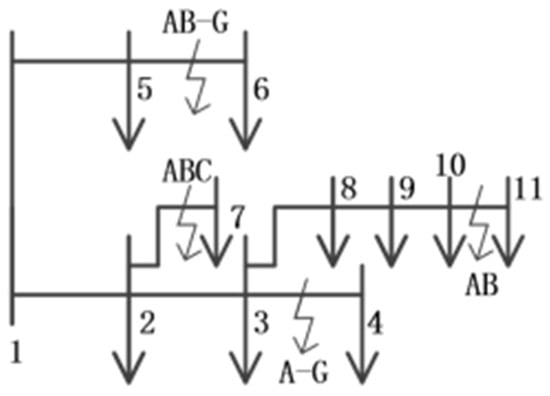
Figure 8.
Simulation model of distribution grids.
4.1. Optimal Allocation
The dynamic BSPO algorithm with constraints is adopted, and the observability of the distribution network and node correlation degree are considered, respectively, in the two constraints, making the collected data more comprehensive and reliable. If x1, x2, …, x11 are used to represent the nodes of the system, then the two constraints can be expressed as Equations (22) and (23), respectively.
According to the fitness function and constraint conditions of DBPSO, there are 6 nodes in the distribution network that need to be equipped with distributed voltage and current sensing devices, namely nodes 2, 3, 5, 6, 9, and 10.
In addition to the IEEE11 node system, the IEEE9 node, IEEE14 node, IEEE24 node, IEEE30 node, IEEE39 node, IEEE57, and IEEE123 node systems are tested. The summary of the test results of DBPSO and Gurobi is shown in Table 7.
Table 7.
Comparison of DBPSO and Gurobi configurations.
In each standard node system, the number of nodes that need to be equipped with measuring equipment determined by the DBPSO algorithm is less than the result of the Gurobi solver. This shows that the DBPSO algorithm can reduce the number of distributed voltage and current sensing devices more effectively and reduce the equipment investment cost on the premise of ensuring the observability of the distribution network.
According to the calculation results of the lower bound of the device configuration, IEEE9, IEEE14, IEEE24, IEEE30, IEEE39, IEEE57, and IEEE123 node systems need to be equipped with 8, 13, 23, 29, 38, 56, and 122 distributed voltage and current sensing devices, respectively. The number of configurations optimized by DBPSO is significantly lower than that corresponding to this lower bound in each node system, which fully demonstrates the outstanding advantages of DBPSO optimization in reducing the number of equipment equipped and effectively reducing the cost of equipment investment.
According to the optimal configuration of the measurement devices of each node system, the proposed DBPSO algorithm based on fixed inertia weight and constraint conditions can greatly reduce the number of distributed voltage and current sensing devices under the condition of satisfying the observability of the distribution network system, so as to reduce the cost of data acquisition and improve the operation efficiency.
4.2. Section Location and Route Selection
The section location of the distribution network system is analyzed by A-G, AB-G, AB, and ABC faults in turn. In the section location algorithm adopted in Chapter 3, it is necessary to compare the similarity between the three fault feature vectors of the positive sequence voltage, zero sequence current and zero sequence impedance Angle of each section comparison point, locate the fault region through the fuzzy C-means algorithm, and on the basis of determining the nodes contained in the fault region, compare the Euclide-distance d1, d2 and d3 between the nodes in the region and various centers. The line on which the node with the smallest Euclidean distance, d1, resides is the faulty line. In the actual measurement situation, the data collected by the voltage and current sensing device is processed by the DSP unit to create a digital signal, and the required fault characteristics are directly output by the communication unit of the Internet of Things terminal.
(1) Single-phase grounding short circuit (fault distance 10 km)
A single-phase grounding short circuit occurs between nodes 3 and 4. When a fault occurs, the fault component of each node and the section location algorithm are shown in Table 8 and Figure 9.
Table 8.
The section location of a single-phase ground fault.
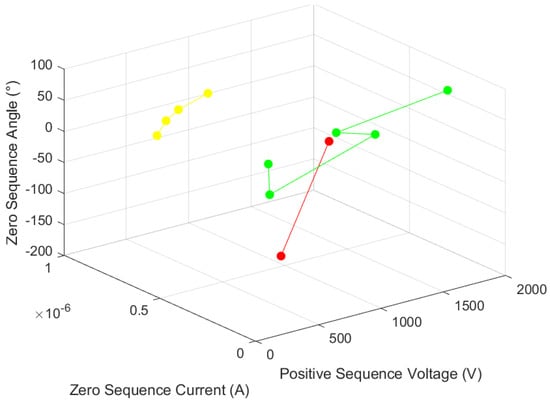
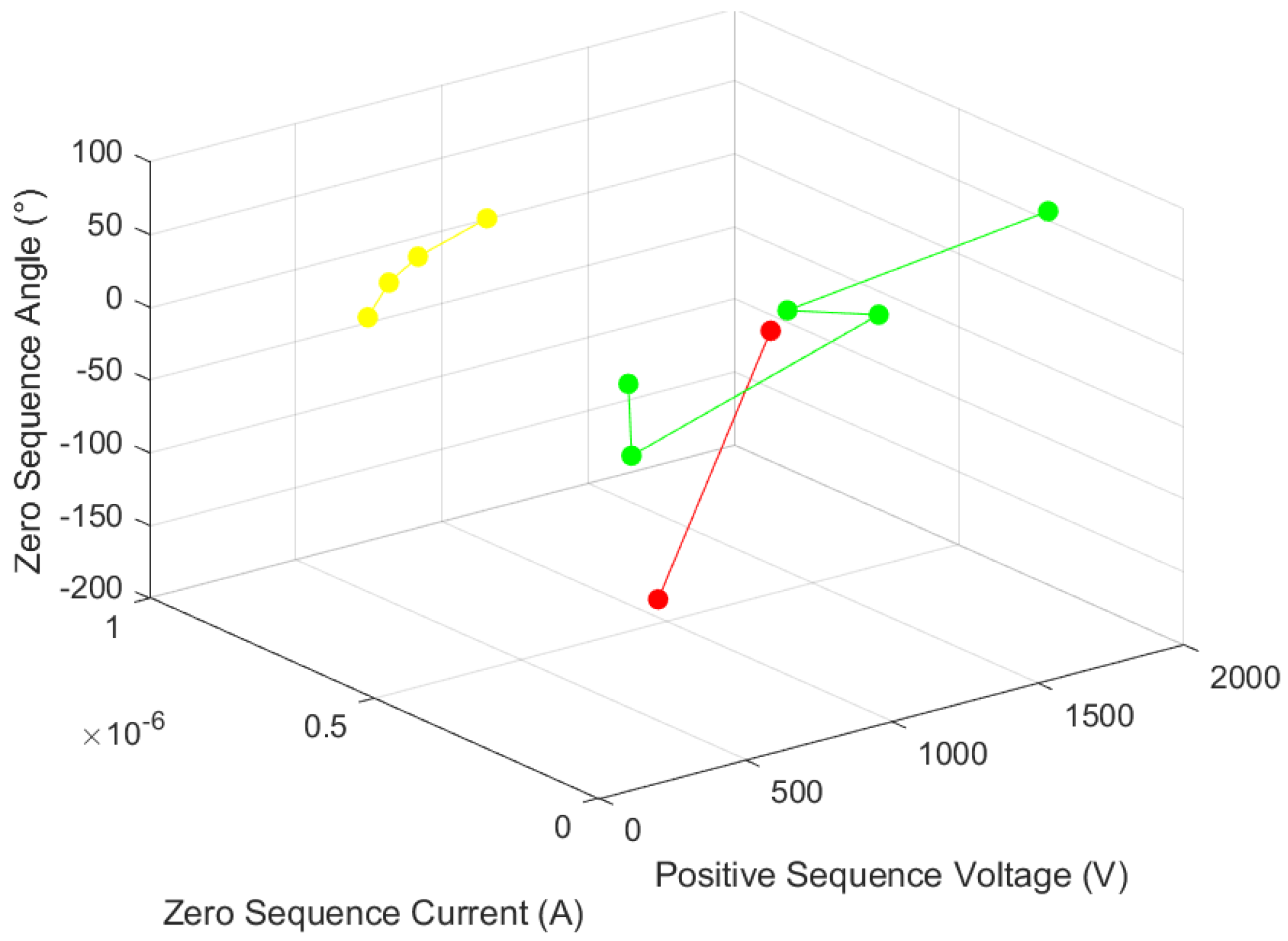
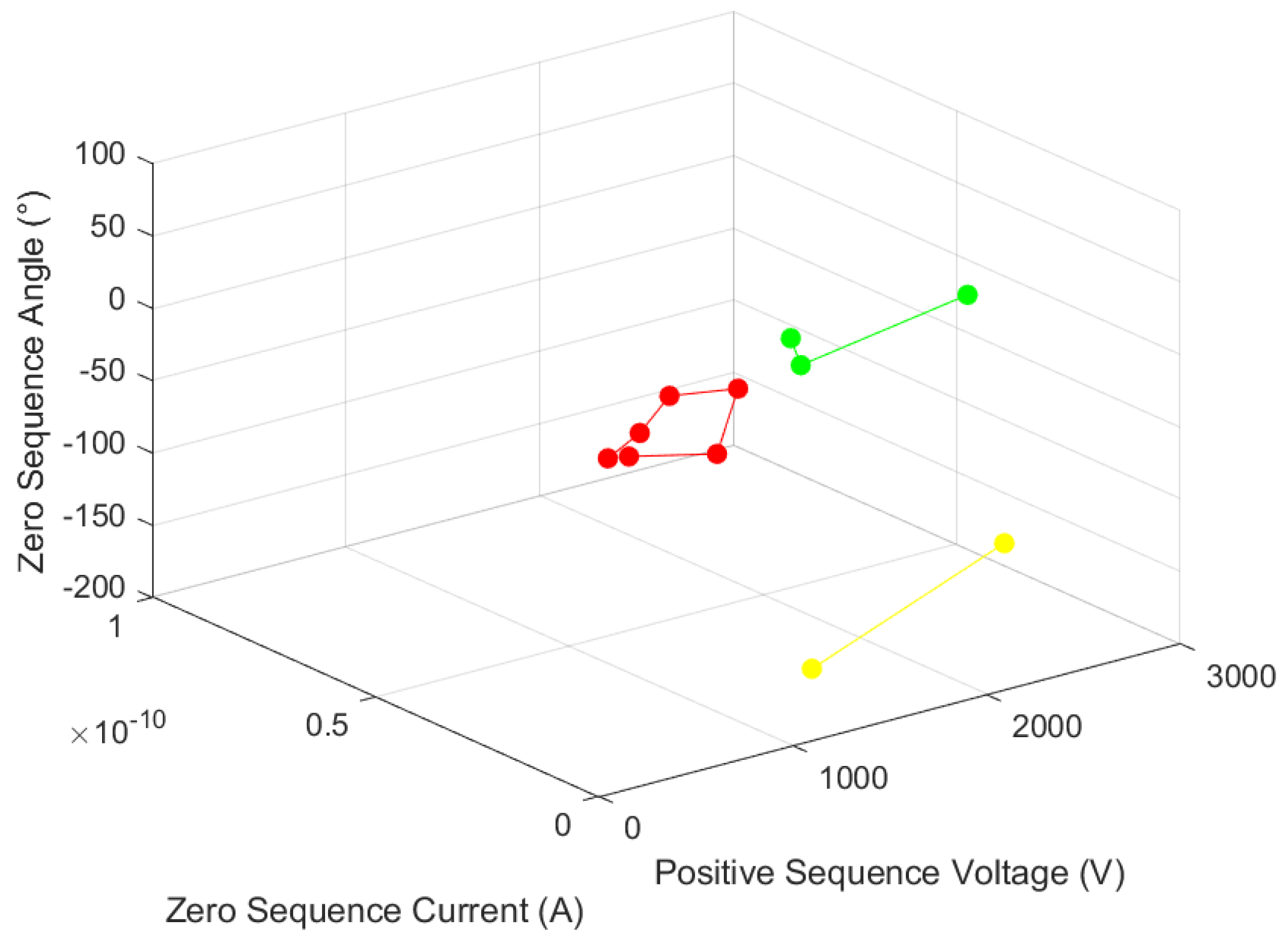
Figure 9.
Result of the division of a single-phase ground fault section.
Red represents fault, yellow represents fault-related, and green represents non-fault. According to the classification, the fault nodes are 3 and 4, the fault-related nodes are 8, 9, 10, and 11, and the non-fault nodes are 1, 2, 5, 6, and 7. The set single-phase grounding fault occurs between nodes 2 and 7, and no line selection is required. The fault area determined by the fault occurrence line algorithm is consistent with the setting condition, and it is proven that the proposed algorithm is effective for locating the fault section of the distribution network.
(2) two-phase ground short circuit (fault distance 30 km)
A two-phase short-circuit occurs between nodes 5 and 6. When a fault occurs, the fault component of each node and the section location algorithm are shown in Table 9 and Figure 10.
Table 9.
The section location of a two-phase ground fault.

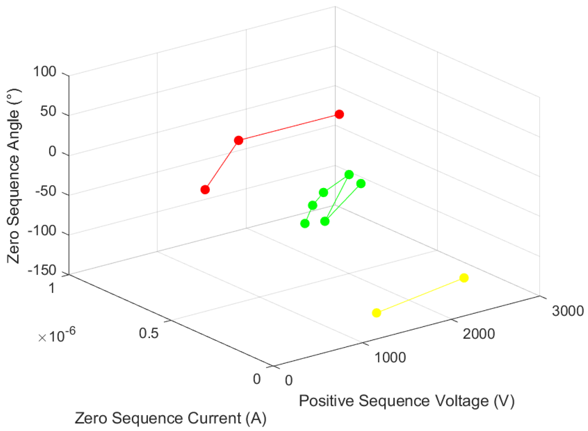
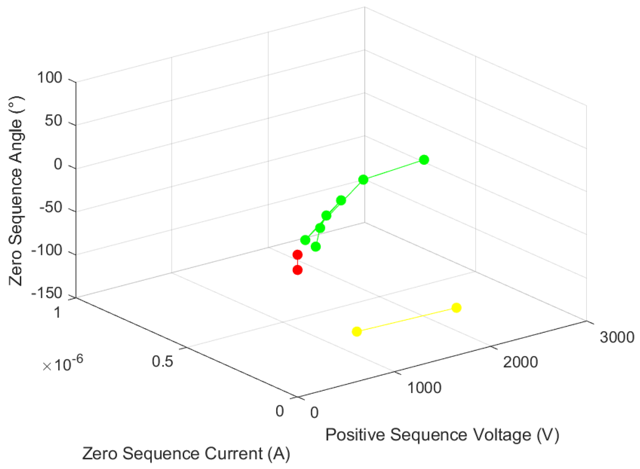
Figure 10.
Result of the division of the two-phase ground fault section.
Red indicates fault, yellow indicates fault-related, and green indicates non-fault. Fault nodes are 1, 5, and 6; fault-related nodes are 3 and 4; and non-fault nodes are 2, 7, 8, 9, 10, and 11. Table 10 lists the fault line selection results.
Table 10.
Results of fault line selection for two-phase grounding.
The two-phase ground fault occurs between nodes 5 and 6, which is consistent with the result of fault line selection. It is proven that the proposed algorithm is effective for fault section location and line selection of the distribution network.
(3) Two-phase short circuit (fault distance 2 km)
A two-phase short circuit occurs between nodes 10 and 11. When a fault occurs, the component of each node fault and the results of the section location algorithm are shown in Table 11 and Figure 11.
Table 11.
The section location of the two-phase short-circuit fault.
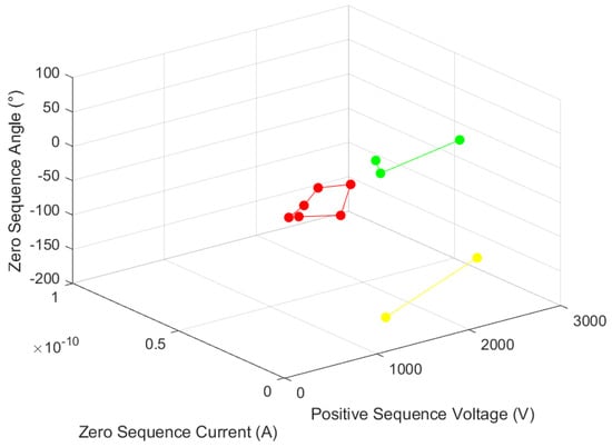
Figure 11.
Result of the division of a two-phase short-circuit fault.
Red indicates fault, yellow indicates fault-related, and green indicates non-fault. Fault nodes are 6, 7, 8, 9, 10, and 11, fault-related nodes are 3 and 4, and non-fault nodes are 1, 2, and 5. Table 12 lists the fault line selection results.
Table 12.
Results of fault line selection for a two-phase short-circuit fault.
The two-phase short-circuit fault occurs between nodes 10 and 11, the fault line selection result is the line from nodes 9 to 11, and the line determined by nodes 10 and 11 is a part of the fault line selection, so the line selection result is valid, and the distance calculation can be carried out in the line determined by nodes 9 and 11. The proposed algorithm is effective for fault location and line selection of the distribution network.
(4) Three-phase short circuit (fault distance 10 km)
A three-phase short circuit occurs between nodes 2 and 7. When a fault occurs, the fault component of each node and the fault segment location algorithm are shown in Table 13 and Figure 12.
Table 13.
The section location of the three-phase short-circuit fault.
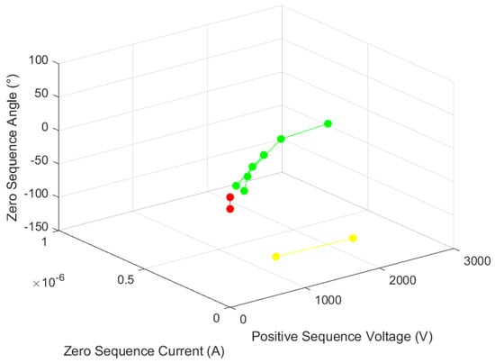
Figure 12.
Result of the division of a three-phase short-circuit fault.
After classification, the fault nodes are 2 and 7, the fault-related nodes are 3 and 4, and the non-fault nodes are 1, 5, 6, 8, 9, 10, 11. The three-phase short-circuit fault occurs between nodes 2 and 7, which is consistent with the location results of the section, and no line selection operation is required. The fault area determined by the fault occurrence line algorithm is consistent. The proposed algorithm is effective for fault location in a distribution network.
5. Conclusions
This paper mainly introduces the DBPSO optimization method based on a distributed voltage and current sensing device and the application of the fuzzy C-means algorithm in fault location and line selection of the distribution network.
Firstly, the BPSO algorithm is compared and explained. By selecting a fixed inertia weight, the constraint conditions of BPSO are increased, the number of iterations is reduced, the operation efficiency is improved, and the measurement range is increased.
Secondly, the theory of the fuzzy C-means algorithm is introduced in detail, and the relationship between membership degree and class center of the fuzzy C-means algorithm is analyzed. Then, the fuzzy C-means algorithm is used to classify the fault information of each node. According to the membership degree of nodes, nodes are divided into three categories: fault node, fault-related node, and non-fault node. This division makes it possible to identify fault areas. Once the fault area is identified, the fault line is further determined by comparing the Euclidean distance.
Finally, the optimal configuration of each node system is verified by MATLAB programming and compared with the configuration solved by Gurobi, demonstrating the advantages of DBPSO in reducing the number and cost of configurations. The IEEE11 node system is used for fault simulation to evaluate the feasibility of the fault location and route selection algorithm. Through the verification, it is found that the algorithm can locate and identify the fault section in the distribution network successfully, regardless of different fault locations and different fault types. It is proven that the combined strategy of DBPSO and FCW is significantly superior to the combined strategy of traditional BPSO and traditional clustering algorithms in terms of the balance of cost and accuracy, verifying the superiority of this strategy.
Although this research has achieved remarkable results in reducing equipment costs and improving positioning accuracy, it is still limited by challenges such as the weakening of high-impedance fault characteristics and the real-time performance of large-scale networks. Future work should focus on feature enhancement algorithms based on machine learning, scalability in large-scale networks, etc., and promote the transformation of hardware from testing to engineering applications.
Author Contributions
Conceptualization, B.L.; Methodology, B.L. and Z.W.; Validation, Z.W.; Investigation, G.Q.; Data curation, G.Q.; Writing—original draft, P.S.; Writing—review & editing, P.S.; Supervision, L.T.; Funding acquisition, L.T. All authors have read and agreed to the published version of the manuscript.
Funding
Yunnan Power Grid Co., Ltd. Electric Power Science Research Institute: 0562002024030301JL00007.
Data Availability Statement
Data is contained within the article.
Conflicts of Interest
Authors Bo Li, Guochao Qian and Lijun Tang were employed by the company Yunnan Power Grid Co., Ltd. The remaining authors declare that the research was conducted in the absence of any commercial or financial relationships that could be construed as a potential conflict of interest.
References
- Chen, Y.; Liu, Y.; Zhao, J.; Qiu, G.; Yin, H.; Li, Z. Medium voltage distribution network expansion planning method based on graph reinforcement learning. Grid Technol. 2025, 1–18. [Google Scholar] [CrossRef]
- Wang, M.; Xu, Y.Q. Transient current fault location of non-fault phase based on wavelet transform and BP network. Power Autom. Equip. 2006, 4, 25–27. [Google Scholar]
- Tao, W.Q.; Cao, H.G.; Yu, N.H.; Li, L.; Yin, S.G.; Bao, X.F. Fault line selection and section location of distribution network based on S transform. Electr. Autom. 2014, 36, 74–77. [Google Scholar]
- Wang, X.W.; Zhang, T.; Tian, S.; Zhang, Y.J.; Li, T.; Cheng, Z.L. Fault section location method for small current grounding system based on approximate entropy. China Electr. Power 2012, 45, 1–6. [Google Scholar]
- Hu, L.X.; Du, W.S.; Li, J.X. A New Fault Recorder Based on DSP + MCU Technology. Relay 2005, 9, 54–57. [Google Scholar]
- Zhang, Y.D.; Jiao, Y.J.; Zhang, J. Design of fault recorder based on embedded system. Relay 2005, 3, 62–65. [Google Scholar]
- Kang, X.N.; Suo, N.J.L. Fault location principle of single-ended electrical quantity frequency domain method based on parameter identification. Chin. J. Electr. Eng. 2005, 2, 25–30. [Google Scholar]
- Qin, D.; Zhang, Z.; Wang, L.; Dam, S.K.; Yang, C.H.; Dong, Z.; Wan, C.; Bai, H.; Wang, F. Co-design of Detection, Actuation, and Control for Solid-state Circuit Breakers in Electrified Aircraft Propulsion System. IEEE J. Emerg. Sel. Top. Power Electron. 2024. [Google Scholar] [CrossRef]
- Qin, D.; Zhang, Z.; Zhang, D.; Xu, Y.; Wan, C.; Lakshmi, R.; Tohid, S.; Dong, D.; Cao, Y. Oscillation Issue and Solution for Solid-State Circuit Breaker Using High Power IGBT Module. IEEE Trans. Ind. Appl. 2024, 60, 765–772. [Google Scholar] [CrossRef]
- Chen, L.; Zhan, Y.D.; Tian, Q.S.; Ma, Z.N. A phase-to-phase short circuit fault location method for 10 kV distribution network. J. Henan Univ. Sci. Technol. (Nat. Sci. Ed.) 2019, 40, 57–61. [Google Scholar]
- Zhang, Y.C.; Su, H.S. A new fault location algorithm for distribution network based on transient zero-mode current. Grid Clean Energy 2013, 29, 29–33. [Google Scholar]
- Li, X.Y.; Liu, Q.; Li, L.Y. Combined fault location method based on single-ended traveling wave method for hybrid lines in distribution network. J. North China Electr. Power Univ. (Nat. Sci. Ed.) 2014, 41, 55–61. [Google Scholar]
- Liu, M.R. A new method of hybrid line ranging in distribution network. Lab. Res. Explor. 2012, 31, 219–222. [Google Scholar]
- Olufunke, A.B.; Yanxia, S.; Peter, A.G. Optimal PV active power curtailment in a PV-penetrated distribution network using optimal smart inverter Volt-Watt control settings. Energy Rep. 2024, 12, 5396–5419. [Google Scholar]
- Wu, S.; Xu, Z.; Zheng, Z.; Cui, J.; Feng, Y. Optimal configuration method of fault location device in low voltage distribution network based on participation. In Proceedings of the 2022 2nd Asia-Pacific Conference on Communications Technology and Computer Science (ACCTCS), Shenyang, China, 25–27 February 2022; pp. 431–437. [Google Scholar]
- Gunawan, R.; Winarko, E.; Pulungan, R. Performance comparison of inertia weight and acceleration coefficients of BPSO in the context of high-utility itemset mining. Evol. Intel. 2023, 16, 943–961. [Google Scholar] [CrossRef]
- Rather, Z.H.; Liu, C.; Chen, P. Optimal PMU Placement by improved particle swarm optimization. In Proceedings of the IEEE Innovative Smart Grid Technologies-Asia, Bangalore, India, 10–13 November 2013; pp. 1–6. [Google Scholar]
- Chen, X.; Chen, T.; Tseng, K.J.; Sun, Y.; Amaratunga, G. Hybrid approach based on global search algorithm for optimal placement of μPMU in distribution networks. In Proceedings of the 2016 IEEE innovative smart grid technologies-Asia (ISGT-Asia), Melbourne, VIC, Australia, 28 November–1 December 2016; pp. 559–563. [Google Scholar]
- Tang, T.; Zhou, Y.; Zeng, X.; Luo, C.; Li, X. Fault location based on FastICA and fuzzy C-means clustering for single-phase-to-ground fault in the compensated distribution network. Electr. Eng. 2023, 105, 4079–4093. [Google Scholar] [CrossRef]
- He, J.T.; Che, R.F.; Meng, Q.M.; Zhang, H. A power grid fault diagnosis method based on wide-area recording data and FCM clustering. Power Autom. Equip. 2019, 39, 179–184. [Google Scholar]
- Yin, H.; Zhang, Y.; Peng, Z. Optimal Sensor Placement Based on Fuzzy C-Means Clustering Algorithm. In Proceedings of the 2018 International Conference on Sensor Networks and Signal Processing (SNSP), Xi’an, China, 28–31 October 2018; pp. 92–98. [Google Scholar]
- Wu, J.K.; Wu, Z.J.; Mao, X.M.; Wu, F.; Tang, H.L.; Chen, L.M. Risk early warning method for distribution system with sources-networks-loads-vehicles based on fuzzy C-mean clustering. Electr. Power Syst. Res. 2020, 180, 106059. [Google Scholar]
- Liang, Z.; Wang, C.; Han, S.; Jan Khan, K.U.; Liu, Y. Classification and susceptibility assessment of debris flow based on a semi-quantitative method combination of the fuzzy C -means algorithm. Factor Anal. Effic. Coeff. 2020, 20, 1287–1304. [Google Scholar]
- Wang, X.Y.; Wang, H.X. Driving Behavior Clustering for Hazardous Material Transportation Based on Genetic Fuzzy C-means Algorithm. J. Math. 2020, 8, 11289–11296. [Google Scholar] [CrossRef]
- Chen, L.; Wang, W.N.; Zhai, Y.Y.; Deng, M.H. Single-Cell Transcriptome Data Clustering via Multinomial Modeling and Adaptive Fuzzy K-Means Algorithm. Front. Genet. 2020, 11, 295. [Google Scholar] [CrossRef] [PubMed]
- He, B.; Peng, L.H.; Shen, J. Research on comprehensive line selection of single-phase grounding fault in distribution network. J. Chongqing Electr. Power Coll. 2019, 24, 3–7. [Google Scholar]
- Zheng, Y.Y.; Zhu, Y.L.; Liu, T.T.; Susan, S. Wind farm single-phase grounding fault section location based on zero-sequence current. J. Syst. Simul. 2019, 31, 1408–1415. [Google Scholar]
- Lin, Z.C.; Liu, X.X.; Wang, Y.M.; Xue, Y.D.; Sun, D.F.; Wang, C. Grounding fault protection of low resistance grounding system based on zero sequence current comparison. Power Syst. Prot. Control 2018, 46, 15–21. [Google Scholar]
- Wu, J.W.; Tong, X.Y.; Liao, X.J.; Zheng, Y.K. Research on new principle of transmission line protection based on zero-sequence differential impedance. Prot. Control Power Syst. 2017, 45, 11–17. [Google Scholar] [CrossRef]


Disclaimer/Publisher’s Note: The statements, opinions and data contained in all publications are solely those of the individual author(s) and contributor(s) and not of MDPI and/or the editor(s). MDPI and/or the editor(s) disclaim responsibility for any injury to people or property resulting from any ideas, methods, instructions or products referred to in the content. |
© 2025 by the authors. Licensee MDPI, Basel, Switzerland. This article is an open access article distributed under the terms and conditions of the Creative Commons Attribution (CC BY) license (https://creativecommons.org/licenses/by/4.0/).