Analysis of Flow Distribution and Heat Transfer Characteristics in a Multi-Branch Parallel Liquid Cooling Framework

Abstract

The parallel multi-branch pipeline system is usually used for fluid transportation and distribution in the cooling of high-power electronic equipment, especially in radar equipment. Using CFD software, a simulation study was conducted to analyze the fluid flow distribution and heat transfer characteristics within a 6 × 5 parallel multi-branch pipe. This study examined how the dimensions of the fluid channels in the liquid cooling system affected the uniformity of flow distribution and the cooling effectiveness of the system for electronic equipment. The deviation from the design flow rate was used as an evaluation criterion to assess flow distribution uniformity across the branches and components of the multi-branch liquid cooling system. After ensuring uniform flow distribution, the overall heat transfer characteristics of the liquid cooling system were analyzed. The main findings are as follows: by adjusting the flow channel dimensions within the system, the overall flow distribution uniformity increased by 10%, with the deviation from the design flow rate in each T/R component remaining within 20%. The 6 × 5 parallel multi-branch cold plate efficiently cools T/R components with heat flux densities of up to 500 W/cm², maintaining the maximum component temperature below 358 K.

1. Introduction

With the progress of science and technology and the improvement of performance requirements, the assembly density and power consumption of radar equipment are getting higher and higher, and the miniaturization and light weight of radar have become an urgent need [1]. The T/R module is a Transmitter and Receiver module; its essence is the signal transceiver accessories. The phased array T/R module refers to the functional module used to receive (referred to as R) and transmit (referred to as T) electromagnetic wave signals of a certain frequency in radar detection or satellite communication systems, and to control the amplitude and phase within the working bandwidth. It is a key component used to control the sending and receiving signals of phased array antennas.

In recent years, the maximum heat flux in the T/R module has been close to 50 W/cm². With the increase in the output and quantity of the T/R module, liquid cooling can be considered as a suitable method [2]. High-efficiency and highly reliable cooling methods are required for radar, and although various cooling methods have emerged, stability and forward movement must be considered. Compared to traditional air cooling, liquid cooling technology offers greater cooling capacity, safety, and reliability. The new cold-plate liquid cooling technology features high thermal conductivity, compact size, and easy high-density integration, presenting broad application prospects in high-power radar cooling systems [3].

The uneven distribution of flow among branches is an inherent characteristic of multi-branch cold plates. Variations in the distance between each branch and the liquid inlet lead to differences in branch resistance and pressure drop, causing uneven flow distribution within the plate. Currently, the key factors influencing the heat transfer capacity of cold plates include the plate structure, material, and cooling medium.

Qian et al. [4] conducted an in-depth study on the topology optimization of fluid channels in the cold plate of active phased array antennas (APAAs) and compared the optimized channels with traditional S-shaped channels. The comparison showed that the optimized channels outperformed traditional designs in most characteristics, especially in temperature uniformity. An et al. [5] studied a hybrid cooling system combining bionic capillary and honeycomb structures. By increasing the contact area between the channels and the battery, they improved thermal conductivity and significantly enhanced cooling capacity. Zuo et al. [6] studied and compared the maximum temperature, temperature difference, and pressure drop of a single S-channel cold plate and a double S-channel cold plate under different conditions. It was found that the maximum temperature of the double S-channel cold plate was close to the maximum temperature of the single S-channel cold plate. The temperature difference of the cold plate with a double S-channel is lower than that of the cold plate with a single S-channel.

Wang et al. [7] researched the cooling effects of microchannel cold plates, revealing that structural optimization, including adjustments to plate thickness, inlet and outlet width, and coolant mass flow rate, significantly impacts maximum temperature and temperature difference, and reduces system pressure drop and energy consumption. Multi-branch flow paths have become an important research area for cold plate cooling. Huo et al. [8] designed a cooling plate with straight microchannels, and they mainly investigated the effects of the number of channels, flow direction, mass flow rate, and ambient temperature on the maximum temperature and temperature difference of the plate. Qian et al. [9] further investigated the cooling performance of the microchannel cooling plate by considering the non-uniform distribution of the coolant. Yang et al. [10] focused on multi-branch parallel fluid loop thermal control technology, widely used in manned spacecraft. A simulation model of six parallel fluid loops was established, deeply analyzing the effects of external heat flow, gravity field, and pipe resistance on flow distribution. The study found that changes in the working fluid’s physical properties due to radiation significantly impacted flow distribution, with branch flow decreasing farther from the inlet and increasing closer to it.

Multi-branch parallel cold plates are widely used in radar systems but still face many challenges. Flow distribution unevenness in multi-branch pipes results in non-uniform coolant distribution within the cold plate, causing inconsistent cooling capacity across the cold plate. For high-power radar cooling, traditional multi-branch parallel cold plates struggle to meet cooling demands in terms of temperature uniformity. At this stage, most researchers and scholars have studied the influence of different structures on the distribution of the single cold plate, but there is less research on the cold plate of the multi-branch pipe. Most scholars merely concentrate on the simplistic branch pipe model cold plates, such as the U-type and Z-type, among others. These cold plates can exert a certain function in the heat transfer of simple cold plates in practical engineering. Nevertheless, it is arduous for them to fulfill the demands of complex cold plate heat transfer and large-power heat sources.

The novelty of this paper lies in the design of a 6 × 5 multi-branch parallel cold plate model. It investigates the flow and heat transfer characteristics of the multi-branch cold plate and conducts a numerical simulation and analysis of its flow and heat transfer properties. This can furnish a theoretical foundation for the design and selection of cold plates in practical engineering. In this paper, the rational pipeline design and flow selection of the multi-branch system can effectively meet the cooling requirements of high-power equipment. Additionally, it optimizes the flow channel design of the cold plate to enhance the heat transfer uniformity of the cold plate.

2. Geometric Model, Mesh Division, and Boundary Conditions

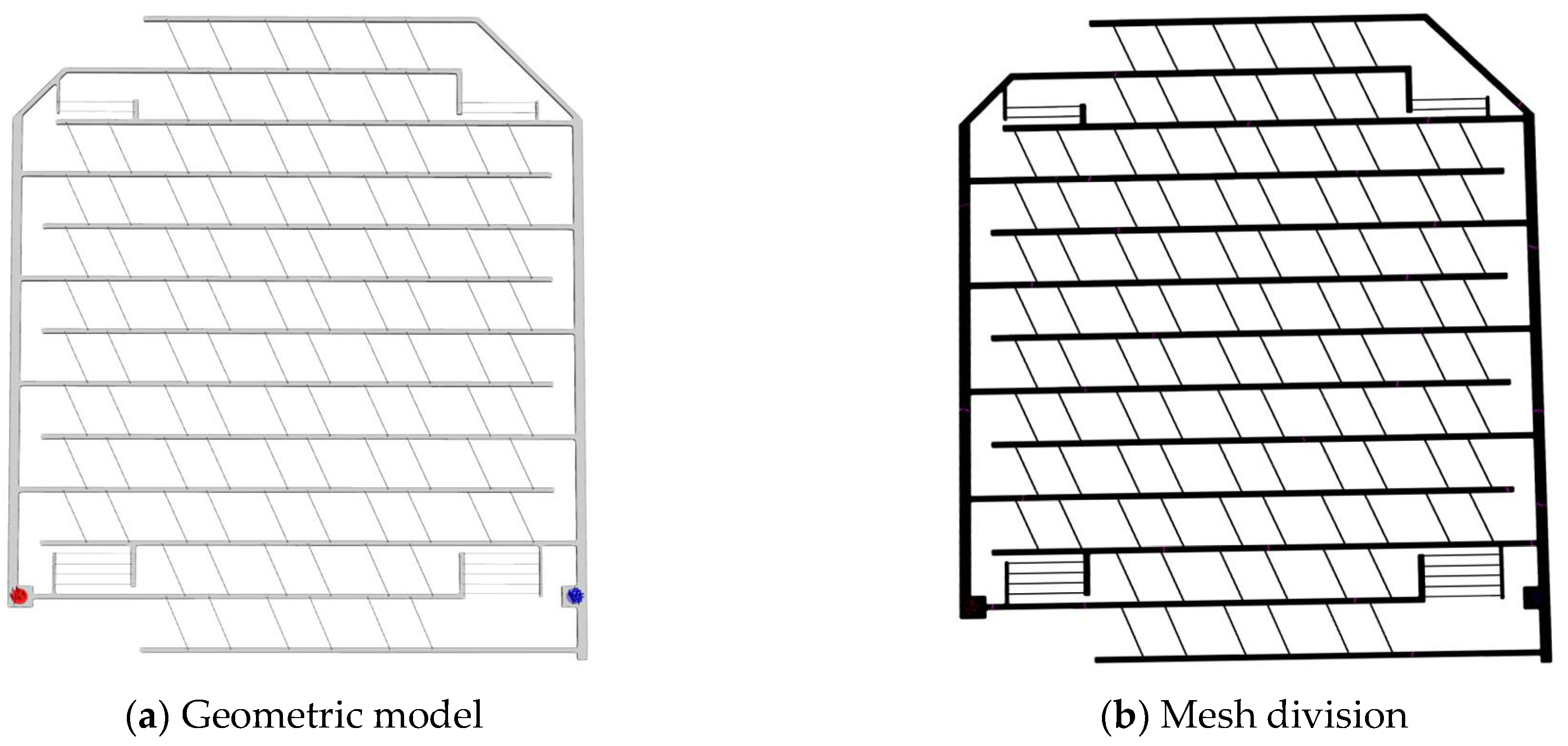
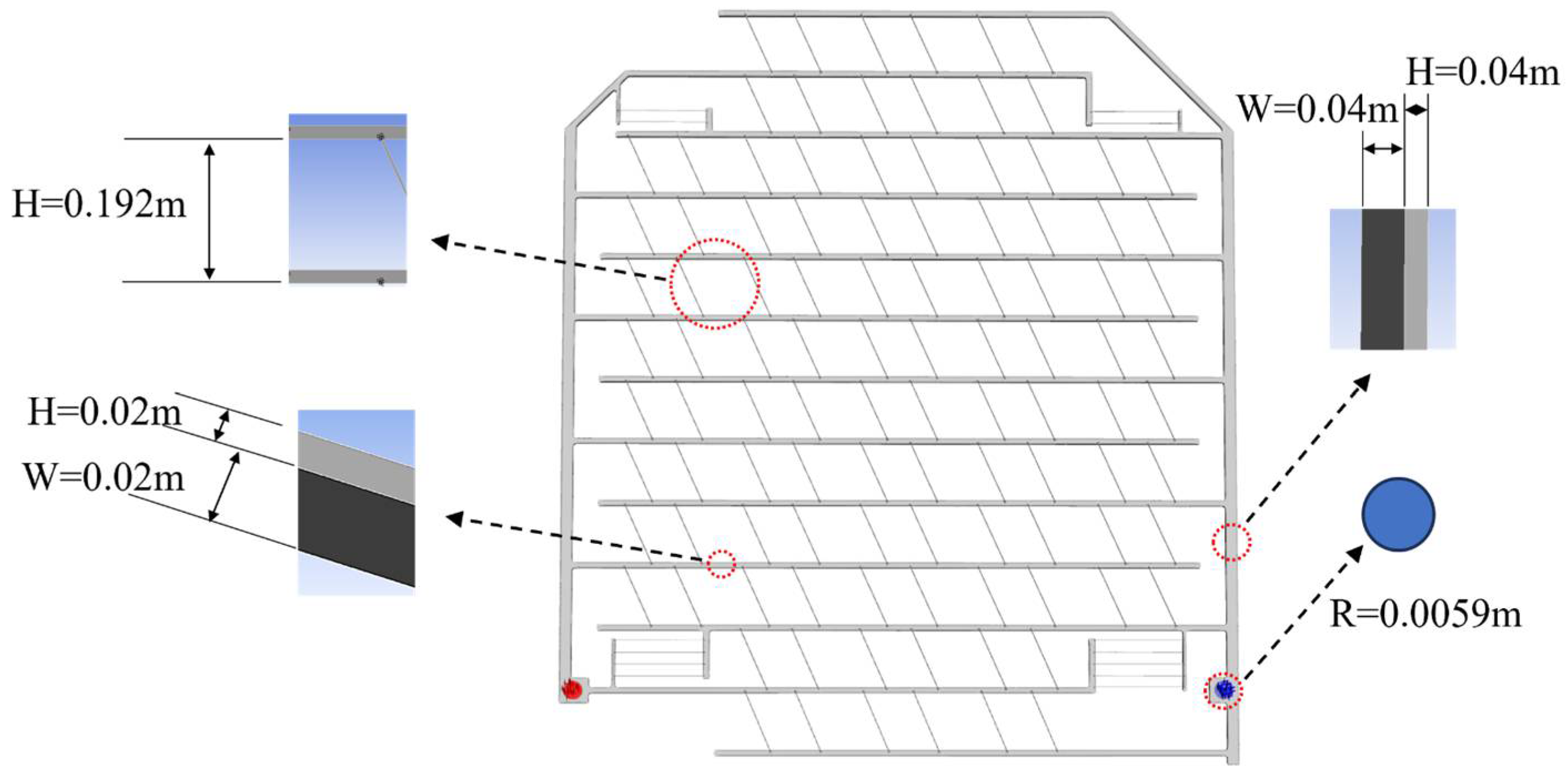
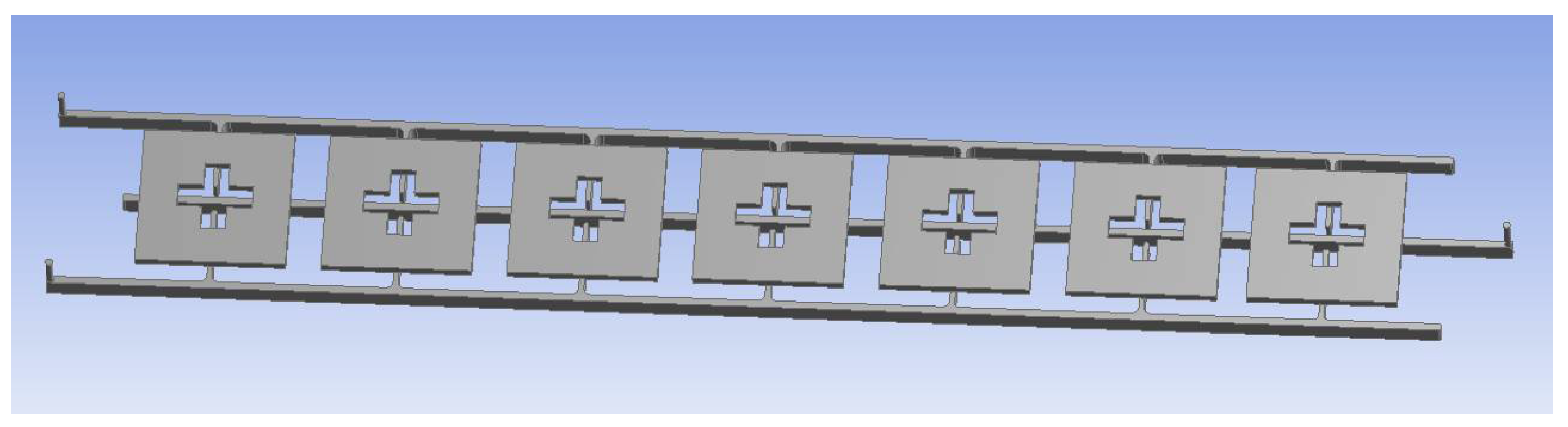
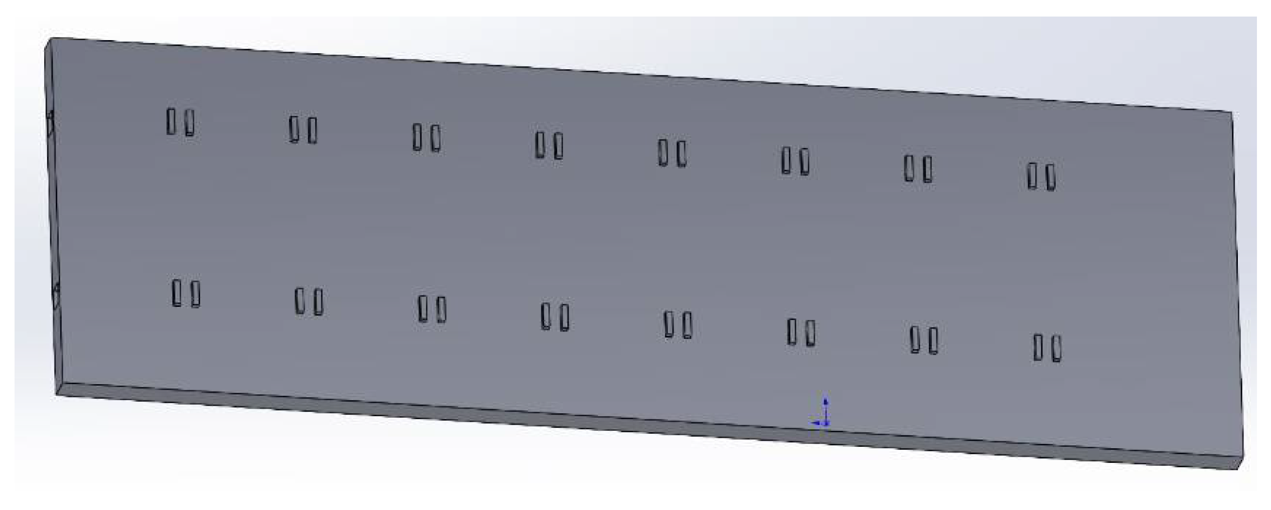
2.1. Geometric Model

The multi-branch cold plate is a crucial liquid cooling method in the radar cooling field, with extensive applications in both military and civilian industries. Investigating the flow and heat transfer characteristics of the 6 × 5 parallel multi-branch cold plate enhances its cooling efficiency and broadens its application scope. Figure 1a illustrates the 3D geometric model of the 6 × 5 parallel multi-branch liquid cold plate. The model comprises 12 layers, including a main liquid supply pipe, a main liquid return pipe, and 13 supply and return branches, specifically seven supply branches and six return branches.

The model is a three-dimensional geometric model that is modeled in Ansys 2022 R1 [11]. In Figure 1a, the blue dot is the inlet of the coolant, and the red dot is the outlet.

The integrated liquid cooling framework is primarily designed for the T/R components, comprising a total of 104 units. Each row of the model contains T/R components, with six components in rows 1, 2, 11, and 12, and ten components in all other rows. The four corners of the model are occupied by distribution components. The spacing between each branch pipe in the model is 0.192 m. Both the inlet and outlet are circular, with a diameter of 0.0059 m. The main supply and return channels have rectangular cross-sections measuring 0.04 m × 0.02 m, while the supply and return branches have square cross-sections of 0.02 m × 0.02 m. Each T/R component consists of a connecting base and a connecting pipe. The cooling liquid channels of two adjacent T/R components form a pair, creating a total of 52 pairs in the liquid cooling framework. Figure 1 is the overall flow channel frame of the large cold plate. Figure 1b shows the meshing results of the entire computational domain. Figure 2 shows the size of the geometric model and marks it in the diagram, which can more intuitively see the size of the geometric model.

The flow and heat transfer of the medium in the pipes involve the mass conservation equation, the energy conservation equation, and the momentum conservation equation:

Mass conservation equation: The increase in the mass of a fluid micro-element per unit time is equal to the net mass flowing into the micro-element during the same period [12].

$$\nabla \overrightarrow{U}={\displaystyle \frac{\partial \mathrm{u}}{\partial x}}+{\displaystyle \frac{\partial \mathrm{v}}{\partial y}}+{\displaystyle \frac{\partial \mathrm{w}}{\partial \mathrm{z}}}=0$$

(1)

In the equation, u, v, and w are the velocity components in the x, y, and z directions, respectively.

Momentum conservation equation:

The physical meaning of the momentum equation is to control the change rate of momentum in the body = surface force (stress) + volume force (gravity, etc.).

$$\rho \left(\partial u/\partial t+u•\nabla u\right)=-\nabla p+\mu {\nabla }^{2}u+f$$

(2)

where ∂ is the Nabla operator $(\partial /\partial \mathrm{x},\partial /\partial \mathrm{y},\partial /\partial \mathrm{z})$ and ∂ 2 is the Laplacian operator $({\partial }^2/\partial {\mathrm{x}}^2+{\partial }^2/\partial {\mathrm{y}}^2+{\partial }^2/\partial {\mathrm{z}}^2).$

At low Re, the viscous force is very large relative to the inertial force $(\rho u·\partial u)$. The influence of the inertia term is relatively small, and the balance of viscous force and pressure gradient mainly drives the flow. The N-S equation is simplified as

$$\rho \partial u/\partial t \approx -\nabla p+\mu {\nabla }^{2}u$$

(3)

When Re is large, the convective inertia term $(\rho u·\nabla u)$ plays a dominant role. The viscous force $\left(\mu {\nabla }^{2}u\right)$ is relatively small in most regions (large scale), but it is crucial at the smallest scale (dissipative scale) for dissipating kinetic energy. The Reynolds-averaged Navier–Stokes (RANS) equations are simplified as follows:

$$\rho \left(\partial \mathsf{ū}/\partial t+\mathsf{ū}•\nabla \mathsf{ū}\right)=-\nabla p^{-}+\mu {\nabla }^2\mathsf{ū}+f-\nabla •\left(\rho u^{\prime }\otimes u^{\prime }\right)$$

(4)

In practical application, the specific expression is shown in Equations (5)–(7):

$${\displaystyle \frac{\partial (\rho u)}{\partial t}}+div(\rho uU)=div(\mu •gradu)-{\displaystyle \frac{\partial p}{\partial x}}+S_u$$

(5)

$${\displaystyle \frac{\partial (\rho v)}{\partial t}}+div(\rho vU)=div(\mu •gradv)-{\displaystyle \frac{\partial p}{\partial y}}+S_v$$

(6)

$${\displaystyle \frac{\partial (\rho w)}{\partial t}}+div(\rho wU)=div(\mu •gradw)-{\displaystyle \frac{\partial p}{\partial z}}+S_w$$

(7)

Energy conservation equation: The heat transfer between the coolant and the cold plate needs to be simulated, so the energy conservation equation needs to be considered.

$${\displaystyle \frac{\partial (\rho T)}{\partial t}}+div(\rho UT)=div({\displaystyle \frac{k}{cp}}gradT)+ST$$

(8)

where T is the temperature, K; C_P is the specific heat capacity of the fluid, J/(kg·K); S_T represents the dissipation term of the fluid.

In the above equation, we assume that the fluid is an incompressible fluid, treat it as a continuous medium, and ignore its molecular structure. The fluid does not undergo phase transition in the cold plate and does not cause mass loss in other ways. In the momentum equation, the non-slip wall is used. It is assumed that the fluid velocity at the solid wall is equal to the wall velocity, that is, the velocity is 0, and the fluid molecules are adhered to the wall. In the energy equation, the radiation heat transfer is assumed to be 0, and the influence of radiation heat transfer is ignored.

2.2. Calculation Method and Boundary Conditions

CFD is used to simulate the flow and flow distribution within the 6 × 5 parallel multi-branch assembly. According to calculation requirements, the turbulence model selected is the k-epsilon-realizable model with an Enhanced Wall Treatment function [13]. Steady-state calculations are performed using the SIMPLE algorithm for the flow field. The discretization scheme for the governing equations adopts a second-order upwind format, and convergence is considered achieved when the residuals of variables in the continuity and momentum equations are below 10⁻⁵ [14]. Turbulence models include the k-ε model, k-ω model, Reynolds stress model (RSM), large eddy simulation (LES), and so on. The k-ε model has a good effect on the fully expanded turbulence (high Reynolds number). The k-ω model has high accuracy in the near-wall region and can analyze low Reynolds number flow without a wall function, which is suitable for boundary layer simulation. The Reynolds stress model (RSM) directly solves the Reynolds stress component and is suitable for complex flows such as strong eddy currents and rotating machinery. Large eddy simulation (LES) is suitable for boundary layer flow and is usually used in aerodynamics. This manuscript is a study of fluid flow in cold plate pipelines which mainly monitors the pressure and flow in the pipeline, and whether the flow in the pipeline is evenly distributed. The model has high accuracy in the near-wall region. It can analyze low Reynolds number flow without a wall function and is suitable for boundary layer simulation. The comparison of boundary layer research is not the focus of this paper. Therefore, the k-ε model is used in the manuscript.

Turbulent kinetic energy (k) transport Equation (9), Turbulent dissipation rate (ε) transport Equation (10):

$${\displaystyle \frac{\partial (\rho k)}{\partial t}}+{\displaystyle \frac{\partial (\rho k{u}_j)}{\partial x_j}}={\displaystyle \frac{\partial }{\partial x_j}}+[(\mu +{\displaystyle \frac{\mu t}{\sigma k}}){\displaystyle \frac{\partial k}{\partial x_j}}]+P_k-\rho \epsilon +S_k$$

(9)

$$\begin{array}{l}{\displaystyle \frac{\partial (\rho \epsilon )}{\partial t}}+{\displaystyle \frac{\partial (\rho \epsilon u_j)}{\partial x_j}}={\displaystyle \frac{\partial }{\partial x_j}}[(\mu +{\displaystyle \frac{\mu t}{\sigma \epsilon }}){\displaystyle \frac{\partial \epsilon }{\partial x_j}}]+C_{\epsilon 1}{\displaystyle \frac{\epsilon }{k}}-C_{\epsilon 2}\rho {\displaystyle \frac{{\epsilon }^2}{k}}+S_{\epsilon }\end{array}$$

(10)

In the equations above, ρ is the fluid density; k is Turbulent Kinetic Energy (the average of the square sum of the fluctuating velocity components), unit: m²/s²; ε is Turbulent Dissipation Rate (the average value of the sum of the squares of the fluctuating velocity gradient multiplied by the kinematic viscosity), unit: m²/s³; t is time; x_j is the space coordinate (j = 1, 2, 3); j is the time-averaged velocity component (j = 1, 2, 3); μ is Molecular Dynamic Viscosity; μ is the turbulent viscosity (Eddy Viscosity), which is calculated by k and ε, where C_μ is an empirical constant. P is the production term of k, which is the main source of turbulent energy and is caused by the time-averaged velocity gradient. Sε is the User-Defined Source Terms.

Ethylene glycol is used as the working fluid, which is treated as an incompressible single-phase flow with constant physical properties. The boundary conditions are set as shown in

Table 1. Boundary condition settings.

Type	Boundary Conditions
Inlet	Mass flow inlet with a mass flow rate of 6.946 kg/s
Outlet	Pressure outlet
Wall	Static non-slip wall
	Adiabatic
	Roughness: Ra3.2
Fluid properties	Viscosity 0.0067 kg/m·s
	Density 1089 kg/m3
Ambient temperature Ambient pressure Runner material	Material: aluminum 297 K 101,325 Pa
	Aluminum alloy

.

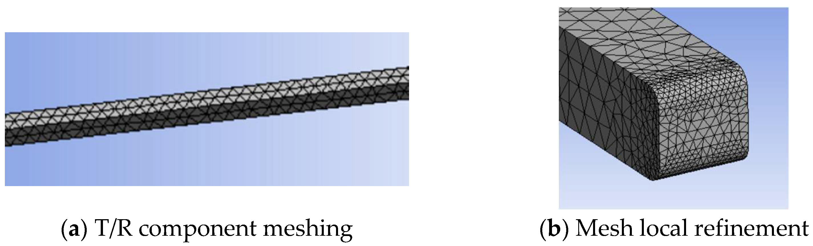
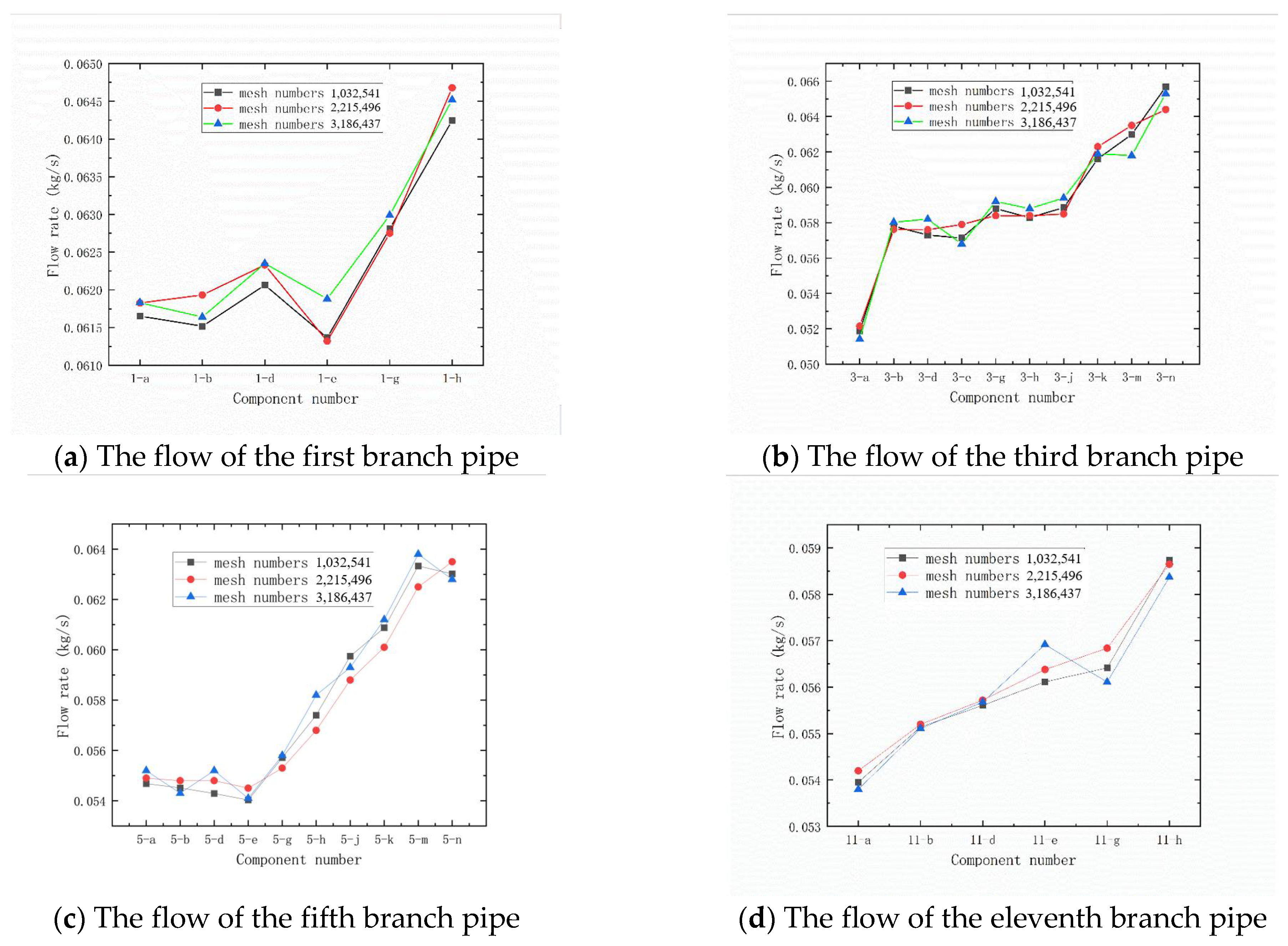
2.3. Mesh Generation and Independence Verification

Mesh generation was conducted using ANSYS Mesh 2022 R1, resulting in a final mesh count of 2,215,496. The minimum element size was 0.00127 m, the maximum area size was 0.146 m, and the average size was 0.003 m. ANSYS Mesh evaluates mesh quality based on criteria such as Element Quality, Skewness, and Orthogonal Quality. Both Element Quality and Orthogonal Quality range from 0 (worst) to 1 (best), with values above 0.75 considered good. Skewness ranges from 0 (best) to 1 (worst) [15].

The global mesh of the model is shown in Figure 1b. Figure 3a focuses on the grid situation of the T/R component. In addition, in order to improve the mesh quality of the key area, the model is also locally refined, as shown in Figure 3b. The average mesh size used in the meshing process is 0.005 m, and the corners of the T/R component and the cold plate model are encrypted so that the accurate results can be calculated better in the calculation.

In the Element Quality and Orthogonal Quality checks, the average Element Quality for all mesh elements was 0.83005, and the average Orthogonal Quality was 0.79, with the minimum values for both metrics exceeding 0.2. The average skewness was 0.239, indicating that the mesh quality satisfies the computational requirements [16].

To investigate the relationship between numerical simulation and grid size, grids with 1,032,541, 2,215,496, and 3,186,437 nodes were selected to simulate the branched pipe flow under the same boundary conditions. Ethylene glycol was used as the fluid, with a mass flow rate of 6.946 kg/s. The flow distributions in the branch pipes are analyzed in Figure 4 for mesh sizes of 1 million, 2 million, and 3 million nodes, respectively. The simulation results indicate that the flow distribution in each branch pipe remains essentially the same at different grid sizes, with the most stable flow observed at 2 million elements. Therefore, the data calculated with a grid of 2 million elements was selected for this analysis.

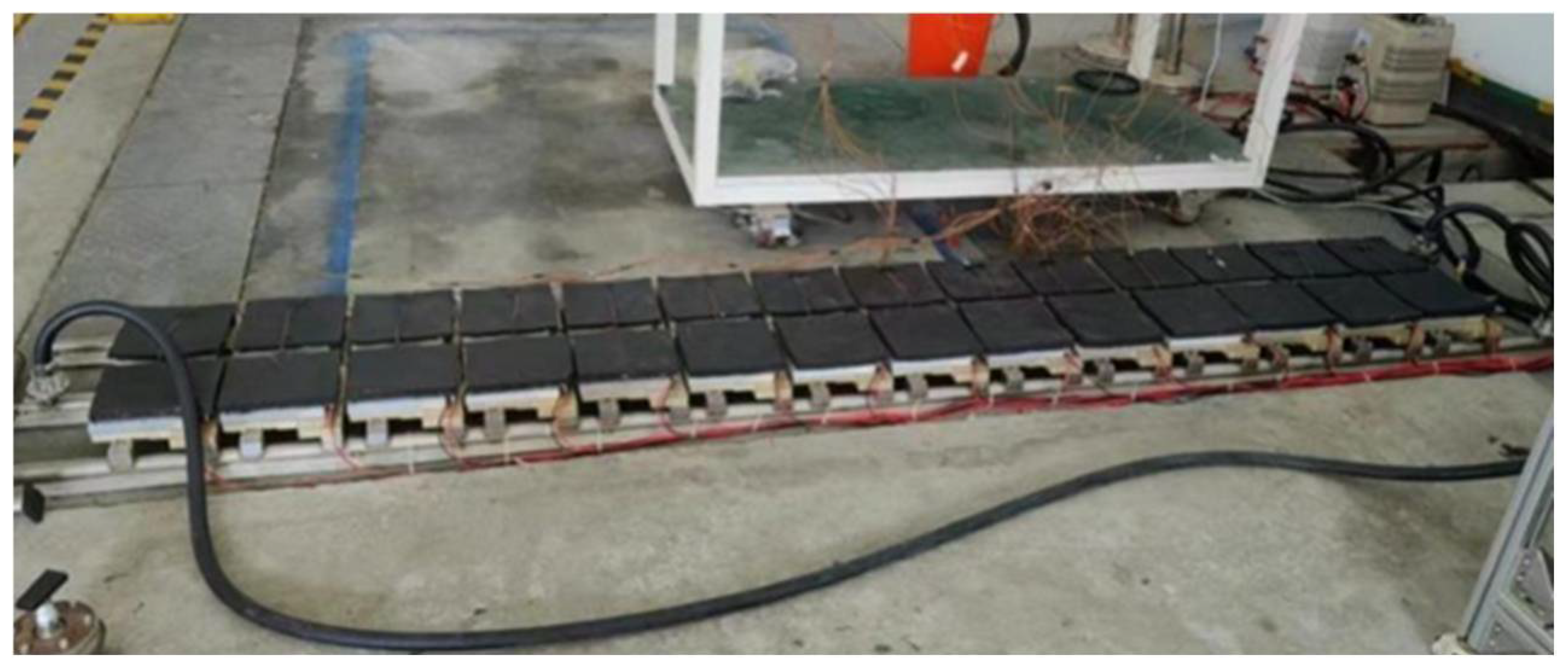
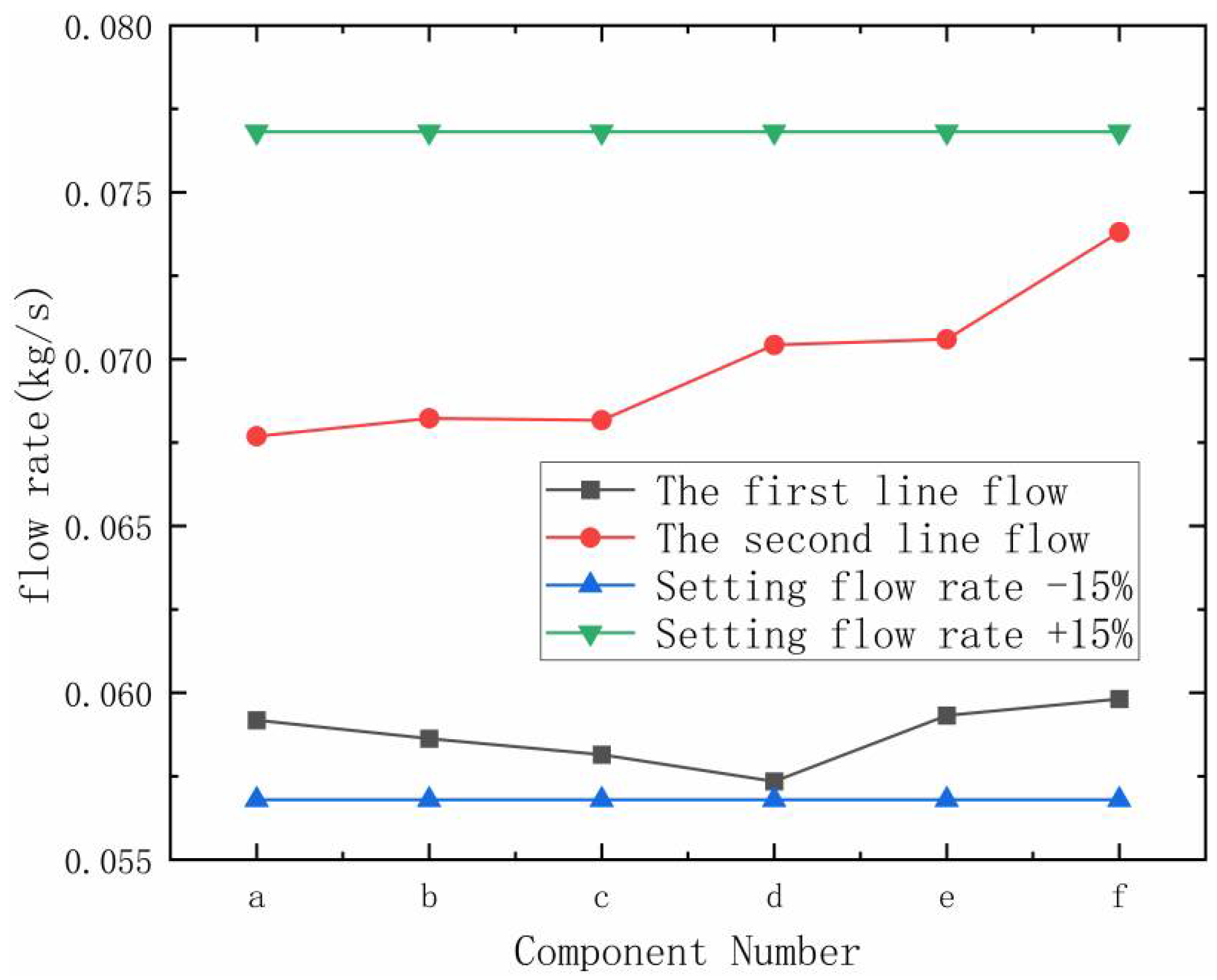
2.4. Experimental Verification

To verify the effectiveness of the numerical simulation, we use the numerical simulation method and model proposed in Section 2.2 to establish a numerical model, whose geometric structure and adiabatic boundary conditions are the same as those described in Reference [17]. The model material in Reference [18] is aluminum, the diameter of the main pipe is 0.015 m, the diameter of the branch pipe is 0.01 m, the thermal power consumption of the cold plate is 100 W, and the coolant is R134a. In the experiment, R134a was used as the cooling medium, and its physical properties are shown in

Table 2. Experimental cooling medium parameters.

Materiality	Parameter Value
Density (kg/m3)	1176
Thermal conductivity (W/m·K)	0.078
Specific heat capacity (kJ/kg·K)	1.461
Kinematic coefficient of viscosity (kg/m·s)	1.8 × 10−4
Temperature (°C)	20

.

The verification geometric model established according to the size of the experimental device in the literature is shown in Figure 5.

The model is verified and analyzed. The 2 × 7 model is divided into seven cold plate areas. We use multiple numerical simulations to verify the relationship between the temperature of the seven cold plates and the numerical simulation. The temperature difference between the numerical simulation and the experiment in the literature is compared. Figure 6 is the experimental verification of the physical model. Figure 7 compares the numerical simulation and experimental results of the seven cold plates, and the maximum error is 6%. Therefore, it can be concluded that the numerical simulation method proposed in this paper is effective.

3. Numerical Simulation Results on Flow Characteristics

3.1. Flow Distribution of the Original Model

The uniformity of flow distribution is a critical issue in cold plate design. Due to the effects of frictional resistance and pressure drop along the path, uneven flow distribution can occur in the cold plate. The flow distribution across the components of the designed cold plate is shown in

Table 3. Flow in T/R components for Group 1.

T/R Component Name	Mass Flow Rate kg/s	Average Value kg/s
1-a	0.0711	0.0736
1-b	0.0788
1-c	0.0710
1-d	0.0733
1-e	0.0735
1-f	0.0738
2-a	0.0685	0.0709
2-b	0.0717
2-c	0.0706
2-d	0.0697
2-e	0.0709
2-f	0.0737

.

Since the number of components in each row varies, the model is divided into three sections for flow description. Rows 1 and 2, located at the bottom of the model, each contain six TR components, referred to as Group 1. Rows 3 through 10 each have ten TR components and are designated as Group 2. Rows 11 and 12, located at the top of the model, each contain six T/R components, referred to as Group 3. As shown in Figure 1, there are 12 T/R components in the bottom two layers of the branch pipe to form Group 1, which is shown in Table 3. The cold plate flow channel is 1–12 rows from low to high, and is named from right to left from a. The T/R pipe name is composed of rows and English letters.

The designed geometric model has a flow rate of 23 m³/h for a total of 104 T/R components, and if the flow rate is distributed uniformly according to each component, the instantaneous flow rate of each component is 0.06679 kg/s.

Figure 8 shows the velocity and pressure states in the supply and return pipelines. In Figure 8a, it is clear that the pressure and velocity are higher at the supply pipeline inlet. The velocity in the main supply pipe decreases from the inlet toward the top of the model, and the flow velocity in the supply branch pipes decreases from the main supply pipe toward the ends of the branches. The flow velocity in the bottommost supply branch is significantly lower than in the second branch from the top at the supply inlet. The figure shows the overall distribution of flow velocity and pressure in the cold plate flow channel. The flow velocity in the T/R component is balanced at the time of design, and the flow velocity and pressure distribution are more uniform. Eddy current occurs at the inlet and outlet of the cold plate, which is caused by the fast flow rate at the inlet and outlet.

Figure 8b displays the pressure contour of the model. It can be observed that the pressure is highest at the supply inlet and lowest at the return outlet. The pressure in the bottommost supply branch of the model is the highest, as this branch is close to the inlet and has no other branches, causing coolant accumulation and increased pressure. The supply side pressure decreases progressively from the bottom to the top of the model, while the return side pressure decreases from the top to the bottom, reaching its minimum at the outlet.

The maximum inlet pressure in the supply pipeline is 178,356.9 Pa, gradually decreasing along the main supply pipe to 145,669.1 Pa at the end of the seventh branch in the cold plate supply model. In the return pipeline, the highest pressure is 82,896.3 Pa at the sixth return branch, while the lowest pressure is −4854.48 Pa at the outlet, resulting in negative pressure. This occurs due to the high flow velocity at the branch outlet, which leads to a pressure reduction.

The first and second rows are the lowest part of the overall model. According to the actual flow of each TR component in the first and second rows, as shown in Figure 9, it can be seen that the flow distribution of each row is such that the flow near the water inlet end is less than the flow near the liquid outlet end, which can be approximated as an increasing flow in sequence. Since the first and second rows are close to the water inlet, the flow and velocity are relatively large, and the flow of the component near the liquid inlet end of the first row exceeds the designed flow by 15%. It can be observed from the geometric model in Figure 1 that the flow of the components in the second row mainly comes from the second liquid supply branch pipe on the right, which is close to the liquid supply port, and the large liquid flow here causes the flow of the b number T/R component in the second row to be too large.

Figure 9b shows the flow distribution of the T/R components in the eleventh and twelfth rows of the model. The two topmost branch pipes are the farthest from the liquid inlet and return liquid port, making them the most disadvantageous branch pipes in the model, with the least amount of coolant flow in the pipes. It can be seen from the figure that the coolant flow in these two branches is mostly less than 15% of the design flow, and the flow of all components is within 20% of the design flow error.

3.2. Flow Distribution of the Improved Model

In response to the phenomenon of excessive flow in the first- and second-row T/R components, the pipes of the first- and second-row liquid supply branch pipes were gradually reduced in size, keeping the thickness of the cross-section of the branch pipe unchanged. The width was half the original branch pipe, making the cross-sectional dimensions 0.01 m × 0.02 m. In contrast, the cross-sectional dimensions of the other branch pipe flow channels are 0.02 m × 0.02 m square, to reduce the flow of the fluid and achieve a uniform flow distribution effect. The details of the model’s gradual reduction are shown in Figure 10.

The modified model is numerically simulated again, and the actual flow distribution of the first row and the second row is analyzed. The actual flow is shown in Figure 10. According to the distribution of the actual flow of each TR component in the first and second rows shown in Figure 11, it can be seen that the error between the flow and the rated flow in these two rows is reduced from 20% to less than 15%. It can be concluded that the diameter of the branch pipe is an important factor affecting the flow distribution.

The middle section of the model consists of rows three to ten, with each row having ten TR components. An analysis and processing of the coolant flow through each component is conducted. In Figure 12a, it can be seen that the component flow from the third to the sixth row is essentially within ±15% of the set flow. In Figure 12b, the actual flow of components a, b, and c in each row is less than the designed flow by −15%.

This indicates that in the distribution of flow in each branch pipe, the actual flow of each TR component from the third to the tenth row has an error within 15% of the rated flow. The flow variation trend of the TR components in each row is consistent with the first and second rows, with the flow increasing sequentially from the liquid supply main pipe towards the liquid return main pipe. Analyzing the overall flow distribution from the third to the tenth row, it can be seen that the flow generally decreases from the third row to the tenth row, meaning that the flow of the TR components in the third row is greater than that in the tenth row.

3.3. The Flow Characteristics with 30% and 50% Concentration of Ethylene Glycol

To explore the influence of ethylene glycol solution concentration on flow characteristics, based on the method described in Section 3.1, a comparative simulation of ethylene glycol aqueous solutions with three volume concentrations of 30%, 50%, and 60% was carried out under the condition of keeping the total inlet flow constant. The flow distribution uniformity of the cold plate was verified and the most unfavorable conditions were identified. The results show significant differences in the hydrodynamic characteristics of solutions with different concentrations. Compared with the 60% concentration solution, the 30% and 50% concentration solutions showed non-uniform flow distribution characteristics in the cooling pipe. The lowest flow area was located in the ninth and tenth rows of the cold plate, and the branch flow showed a non-linear trend of decreasing first and then rising. This phenomenon indicates that the change in solution concentration will significantly affect the flow stability of the system, and it is necessary to consider the influence of concentration gradient on the distribution uniformity in the thermal management design. Here, the flow distribution data of the cold plate with a volume concentration of 30% are shown in

Table 4. Flow distribution of cold plate with 30% volume concentration.

Numbering	a	b	c	d	e	f	g	h	i	J
1	0.0659	0.0749	0.0671	0.0698	0.0700	0.0709	/	/	/	/
2	0.0642	0.0681	0.0647	0.0661	0.0663	0.0696	/	/	/	/
3	0.0579	0.0643	0.0622	0.0657	0.0628	0.0638	0.0653	0.0664	0.0711	0.0725
4	0.0631	0.0624	0.0675	0.0662	0.0663	0.0701	0.0695	0.0702	0.0719	0.0712
5	0.0492	0.0560	0.0561	0.0581	0.0609	0.0596	0.0602	0.0645	0.0660	0.0636
6	0.0541	0.0579	0.0605	0.0537	0.0619	0.0644	0.0622	0.0657	0.0658	0.0688
7	0.0503	0.0509	0.0517	0.0556	0.0548	0.0540	0.0560	0.0587	0.0621	0.0650
8	0.0522	0.0594	0.0596	0.0554	0.0608	0.0570	0.0565	0.0588	0.0602	0.0624
9	0.0493	0.0558	0.0506	0.0567	0.0560	0.0593	0.0575	0.0577	0.0604	0.0643
10	0.0548	0.0524	0.0566	0.0557	0.0573	0.0560	0.0604	0.0601	0.0583	0.0616
11	0.0527	0.0552	0.0588	0.0580	0.0605	0.0507	/	/	/	/
12	0.0574	0.0547	0.0566	0.0588	0.0613	0.0607	/	/	/	/

.

4. Numerical Simulation Results on Heat Transfer Characteristics

The heat source in the radar mainly comes from the signal transceiver, power amplifier, and other T/R components [17]; usually, a phased array radar contains tens of thousands of T/R components, so how to dissipate this part of the heat promptly has become the main point of research on radar cooling. Some data show that the chip temperature rises by 5 K every time, the reliability of its work will be reduced by 5%, and the higher temperature will seriously damage the life of the component.

Figure 13 shows the heat source arrangement of the T/R module of the 6 × 5 multi-branch cold plate model, which is taken from the 6 × 5 parallel multi-branch cold plate model. There are two DC coolant pipes in the cold plate, and the T/R module is installed on the upper part of the coolant channel. The size of the model cold plate intercepted in Figure 13 is 192 mm × 60 mm × 5 mm. The cross-sectional area of the coolant channel is 3.5 mm × 3.5 mm square of the DC channel. The size of the T/R module is a 4 mm × 1 mm × 1 mm chip block. A total of 16 sets of heat sources are set, and the number of heat sources in each group is the same. Each group of heat sources is composed of two T/R module chip blocks.

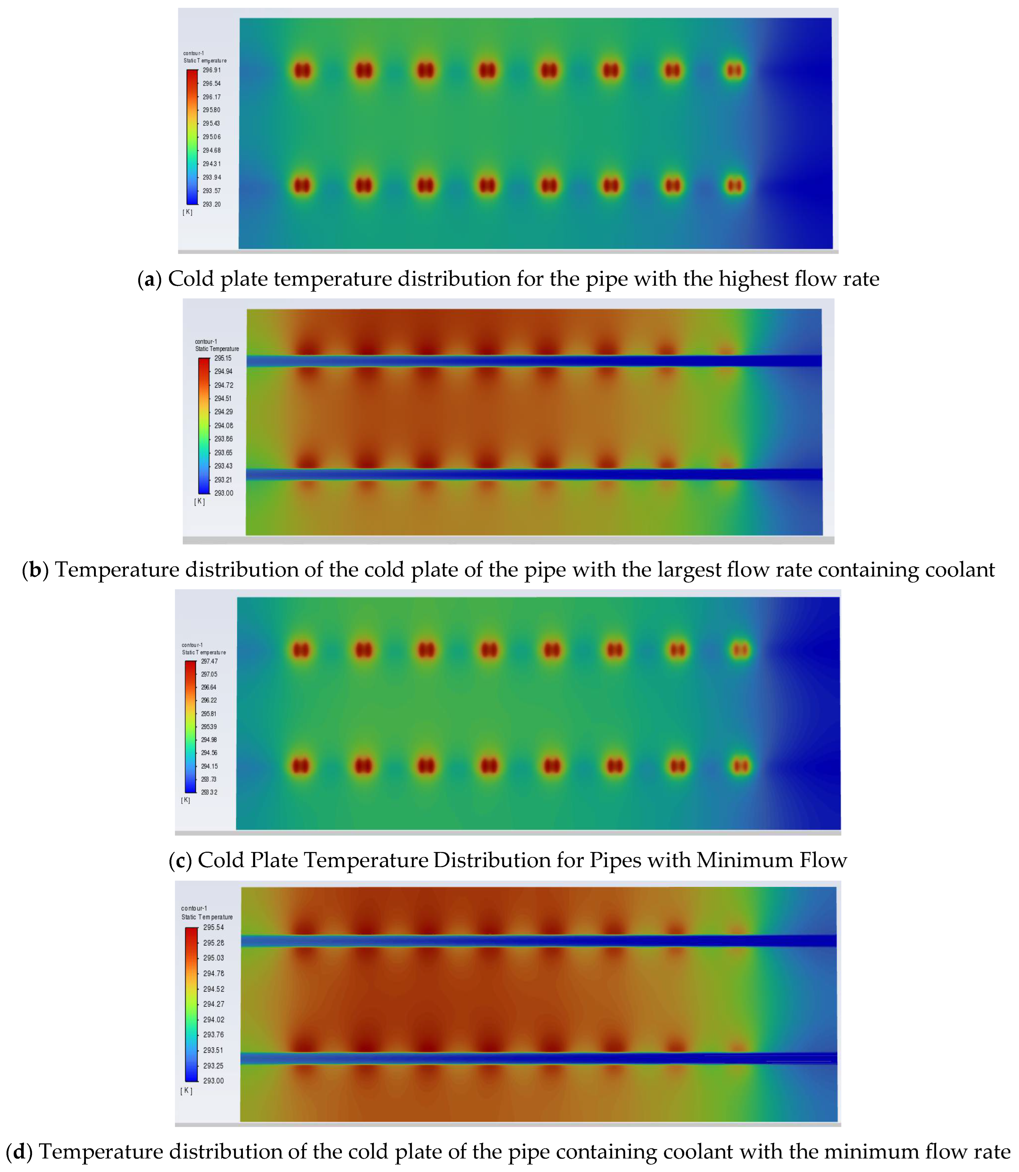
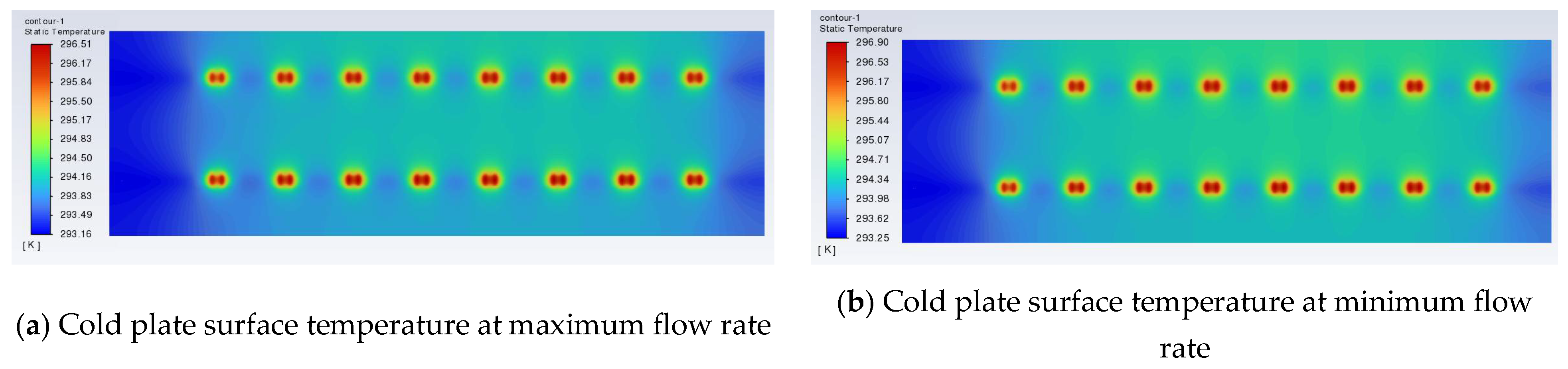
4.1. Different Volume Concentrations of Ethylene Glycol Aqueous Solution

This summary analyzes the influence of different cooling media on the heat transfer characteristics of the cold plate. Here, different concentrations of ethylene glycol aqueous solution are used as the cooling medium, and the commonly used ethylene glycol concentration is between 30% and 60%. Higher or lower concentrations will affect the working efficiency of the cooling medium. Too low a concentration will increase viscosity, reduce heat dissipation efficiency, and increase pump load. Here, three working conditions are selected; the concentration of ethylene glycol in extreme cases is 30% and 60%, and the concentration of ethylene glycol in normal cases is 50%, as different working conditions to explore the effect of different concentrations of ethylene glycol solution on the cooling effect at 20 °C. The physical parameters of different concentrations of the ethylene glycol solution are shown in

Table 5. Physical parameters of different concentrations of ethylene glycol aqueous solution at 20 °C.

Volume Concentration	Density	Specific Heat Capacity	Dynamic Viscosity	Thermal Conductivity
Unit	kg/m3	J/(kg·K)	mPa·s	W/(m·K)
60%	1086	3084	5.38	0.349
50%	1073	3281	3.94	0.380
30%	1045	3645	2.2	0.453

.

4.1.1. Ethylene Glycol Aqueous Solution of 60% Volume Concentration

This model’s heat dissipation method adopts forced liquid cooling. The fluid mass’s inlet temperature is set to 20 °C. The inlet method is a mass flow inlet, whose inlet mass is the mass flow rate passing through the model component in the Fluent simulation. The outlet is set to a pressure outlet, and the cold plate material is aluminum alloy.

The volume concentration of the cooling medium is set to 60%. The simulation of the cold plate is carried out by setting the heat flow density to 48 W/cm², setting the boundary conditions in Fluent, and setting the inlet mass flow rate of the two coolant pipes to 0.0711 kg/s and 0.0788 kg/s, respectively (this value is the mass flow rate passing through the first layer of the T/R assembly in the simulation of the 6 × 5 parallel multi-branch cold plate model, which is the largest mass flow rate in the cold plate model, representative of the cold plate model). The number of iteration steps is set to 500, and the simulation results are obtained, in which the temperature clouds of the cold plate and T/R components are shown in Figure 14a, and the temperature profiles of the cold plate with coolant are shown in Figure 14b.

We can see from Figure 14a in the T/R component a heat flow density of 48 W/cm², the cold plate on the T/R component cooling, cold plate overall temperature uniformity, the highest temperature of the T/R component 299.9 K, the lowest temperature of 296.9 K, the highest and lowest temperature difference of 2.95 K; from Figure 14b can be seen at the right end of the cold plate temperature is low, 293 K, is the set inlet temperature, from right to left observation can be seen that the temperature of the cold plate gradually increased, indicating that with the flow of coolant, the cooling capacity of the cold plate gradually decreased. In the cooling process of the cold plate, the temperature of the coolant is unchanged, which shows that the cold plate can deal well with the radar heating in the case of 48 w/cm² heat flow density.

Observing the cooling capacity of the cold plate in the most unfavorable case for the 6 × 5 parallel multi-branch cold plate, the temperature cloud is shown in Figure 14c,d. The flow rates of the two cooling pipes passing through the cold plate in the most unfavorable case are 0.0598 kg/s and 0.0560 kg/s. Comparing them with the cold plate with the largest mass flow rate, it is found that the maximum temperature of the T/R assembly with the smallest flow rate is 300.31 K, which is 0.45 K higher than the temperature of the cold plate at the time of the largest flow rate, and there is no temperature difference, which illustrates the homogeneous nature of the cooling capacity of the cold plate. Comparing the temperatures of the cold plate in Figure 14b,d, it can be found that the temperature distribution of the cold plate with the smallest flow rate along the direction of the coolant is significantly higher than that of the cold plate with the larger flow rate, which indicates that the coolant with different flow rates will cause different cooling effects.

4.1.2. Ethylene Glycol Aqueous Solution of 50% and 30% Volume Concentration

The maximum flow rate of the aqueous ethylene glycol solution with a volume concentration of 50% appeared in the first row of the cold plate, and the flow rates of the two adjacent T/R components were 0.0720 kg/s and 0.0727 kg/s. The minimum flow rate appeared in the eleventh row of the stubs, and the flow rates of the two adjacent components were 0.0537 kg/s and 0.0561 kg/s. The maximum flow rate of the 30% volume concentration of ethylene glycol solution appeared in the stubs. The maximum flow rate of the aqueous glycol solution with a volume concentration of 30% appeared in the third row of the cold plate, with flow rates of 0.0711 kg/s and 0.0725 kg/s in the two neighboring T/R assemblies, while the minimum flow rate appeared in the tenth row of the branch, with flow rates of 0.0524 kg/s and 0.0548 kg/s in the two neighboring assemblies. The reasons for the different locations of the maximum and minimum flow rates of different concentrations of ethylene glycol solutions are the different physical parameters of different volume fractions of ethylene glycol solutions, resulting in different flow resistance and flow pressure, which ultimately lead to different flow characteristics of the fluids in the cold plate. The flow rate of each component is within 20% error of the average flow rate.

The method in Section 4.1.1 was used to demonstrate the effect of a 50% volumetric concentration of aqueous ethylene glycol and a 30% volumetric concentration of aqueous ethylene glycol on the heat exchange of the cold plate. The heat transfer method is forced liquid cooling with the heat flow density set to 48 W/cm².

Figure 15a,b show the temperature changes on the surface and inside of the cold plate when the flow rate in the cold plate assembly is at a minimum of 50% glycol concentration, and the maximum temperature of the cold plate is 297.76 K and the minimum temperature is 293.56 K under the power of heat source of 48 W/cm². Figure 15a shows the temperature change on the contact surface between the cold plate and the T/R module, and Figure 15b shows the temperature inside the cold plate. It can be seen from Figure 15b that the heat distribution of the whole cold plate is relatively uniform, and the temperature of the coolant in the cold plate is low, which can exchange heat with the cold plate well and take away the heat in the cold plate. Figure 15c,d show the cooling medium for the 50% concentration of glycol solution in the cold plate at the maximum flow rate of the cold plate temperature distribution. Figure 15c shows the cold plate and the T/R components of the temperature distribution of the contact surface; Figure 15d is the temperature distribution inside the cold plate, the maximum temperature of 297.28 K, the lowest temperature of 293.38 K, and the temperature difference between the cold plate of 4 K.

The same method was used to verify the effect of 30% concentration of aqueous ethylene glycol solution as a cooling medium on the heat exchange of the cold plate. It was found that the cooling effect of 30% concentration of glycol solution under the heat source power of 48 W/cm² was the same as that of 50% concentration of glycol aqueous solution. The maximum temperature of the surface of the cold plate at the maximum flow rate is 296.51 K, and the maximum temperature of 50% concentration of ethylene glycol solution is 297.28 K, with a difference of less than 1 K, which indicates that the concentration of ethylene glycol aqueous solution does not have much influence on the heat exchange effect of the cold plate under the heat source power of 48 W/cm².

Figure 16 shows the temperature distribution of this surface of the cold plate when 30% concentration of glycol aqueous solution is used as the cooling medium; the temperature distribution inside the cold plate is the same as that inside the cold plate with 50% concentration of glycol aqueous solution, and the temperature distribution is more uniform. Figure 16a shows the surface temperature of the cold plate with the maximum flow rate of components in the cold plate when 30% ethylene glycol aqueous solution is used as the cooling medium. Figure 16b shows the surface temperature of the cold plate with the minimum flow rate of components in the cold plate, the maximum temperature of the components with the maximum flow rate of components is 296.51 K, and the maximum temperature of the components with the minimum flow rate of components is 296.9 K, with a difference of only 0.39 K; this means that the temperature difference of the cold plate is small, the temperature distribution of the cold plate is more uniform, and there will be no local hot spot, which can achieve the effect of uniform heat transfer.

In summary, under the designed flow rate, the cold plate can take away the heat generation of the T/R component almost completely, the temperature rise of the component is not large, and the heat flow density of the T/R component of 48 W/cm² cannot fully play out the cooling capacity of the 6 × 5 parallel multi-branch pipe cold plate.

At this stage, the heat flow density of the radar module is unevenly distributed from tens to thousands of W/cm² [1], and the cooling capability of the 6 × 5 parallel multi-branch cooling plate is verified again with the typical centralized heat flow density here. The simulation model is established with the method in Section 1 of this paper, and the results are shown in

Table 6. Temperature of T/R components at different heat flow densities.

Name	Heat Flow Density (W/cm2)
numerical value	125	300	500	1000
Maximum temperature of the T/R module K	312.7	338.7	358.2	445.9
Minimum temperature of the T/R module K	302.5	316.3	331.8	370.2
Maximum temperature of cold plate K	304.6	320.9	339.5	386.6
Minimum temperature of cold plate K	293.8	295.3	296.3	299.6

.

4.2. Cooling Effect of the Cold Plate at Different Powers

The cold plate is designed for radar cooling requirements. When the radar system needs to operate under extreme environmental conditions, 60% concentration of ethylene glycol aqueous solution is used as the cooling medium [19] (with excellent thermal conductivity and low-temperature stability). By simulating different heat source power conditions, the system evaluates the heat dissipation performance of the cold plate under different heat load conditions, which can also provide a theoretical basis for other heat source cooling.

According to the simulation results, it can be found that when the heat flow density of the T/R component is 500 W/cm², the maximum temperature of the T/R component is 369.2 K, which has exceeded the normal temperature of the radar operation, and the radar component can still work under this temperature, but the radar’s working reliability and life are seriously affected. When the heat flow density of the T/R component is 1000 W/cm², the maximum temperature of the T/R component is 445.95 K, which seriously exceeds the safe working temperature range of the radar, indicating that the 6 × 5 parallel multi-branch cold plate can meet the 500 W/cm² and below heat flow density components under the design flow rate but cannot meet the 1000 W/cm² heat flow density of the T/R component. The are two reasons for this: one is the runner in the branched cold plate is DC channel, and the second is the coolant flow rate in the runner is too fast, leading to the cold plate not carrying out sufficient heat exchange with the coolant. For heat flux densities exceeding 1000 W/cm², as discussed in this paper, modifications to the placement of the heating element or the width of the cold plate channel can enhance heat transfer. These adjustments increase the heat transfer area, thereby improving the efficiency of heat removal.

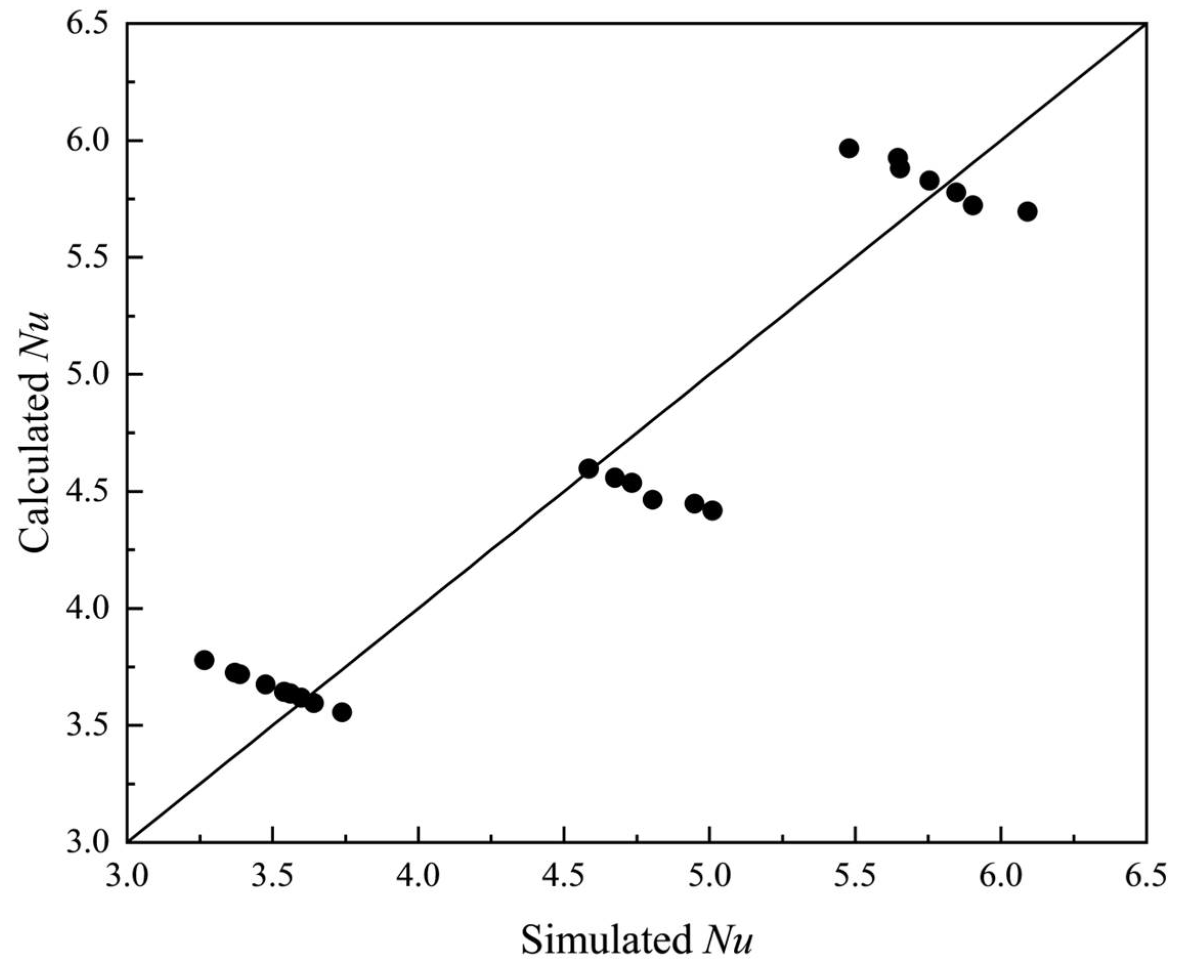
4.3. Analytical Heat Transfer Equation

In heat transfer, the Nusselt number Nu is a dimensionless number describing the strength of convective heat transfer [20]. Through numerical simulation, Nu suitable for this model is analyzed in depth, and an accurate fitting formula of Nusselt number (Nu) is established, which can provide a reliable prediction for engineering applications and theoretical research. The Prandtl number (Pr) is a dimensionless number in fluid mechanics and heat transfer, which is used to describe the important parameters of momentum diffusivity and thermal diffusivity of different concentrations of ethylene glycol. According to different flow rates, multiple sets of Reynolds number (Re) are calculated, and then the Nusselt number (Nu) is calculated by the Nusselt number definition (Nu). The relationship between the Nusselt number (Nu), Reynolds number (Re), and Prandtl number (Pr) is fitted in the origin.

Table 7. Reynolds number and Nusselt number under different flow rates.

Flow Velocity kg/s	Re	Nu
0.0537	6974.026	5.479
0.0538	2857.142	3.265
0.0561	2979.288	4.585
0.0561	7285.714	5.647
0.0588	3122.676	3.370
0.0588	7636.363	5.653
0.0592	3143.919	4.675
0.0595	3159.851	3.387
0.0610	3239.511	4.733
0.0622	8077.922	5.755
0.0657	8532.467	5.846
0.0675	3584.705	4.804
0.0677	3595.326	3.539
0.0685	3637.812	3.560
0.0691	3669.676	4.948
0.0698	9064.935	5.904
0.0706	3749.336	3.598
0.0719	9337.662	6.091
0.0721	3828.996	5.010
0.0735	3903.345	3.641
0.0788	4184.811	3.738

shows the different flow velocities randomly selected in the model and the Reynolds number (Nu) and Nusselt number (Nu) at this time [21].

The formulas used in the calculation are the Reynolds number definition formula, the Nusselt number definition formula, and the Prandtl number definition formula, which are Equation (11), Equation (12), and Equation (13), respectively.

The Reynolds number is defined as follows:

$$\mathrm{Re}={\displaystyle \frac{\rho \mathrm{u}L}{\mu }}$$

(11)

In the equation,

• $\mathsf{\rho }$—Density, kg/m³;
• u—Flow rate, m/s. The average velocity in the cold plate pipe is used here;
• L—Characteristic length, m. The characteristic length is calculated by the size of the cooling pipe;
• $\mu$—Kinematic viscosity, Pa·s.

The definition of the Nusselt number is shown in Equation (12):

$$N\mathrm{u}={\displaystyle \frac{\mathrm{h}L}{\mathrm{k}}}$$

(12)

In the equation,

• $h$—Convective heat transfer coefficient, W/(m²·K). The convective heat transfer coefficient is calculated by the heat flux and its average temperature difference, which is the average convective coefficient of the cold plate;
• $L$—Characteristic Length, m. The characteristic length is calculated by the size of the cooling pipe;
• $k$—Thermal Conductivity, W/(m·K).

The definition formula of the Prandtl number is shown in Equation (13):

$$\mathrm{Pr}={\displaystyle \frac{\gamma }{\alpha }}$$

(13)

In the equation,

• $\gamma$—Kinematic viscosity, m²/s;
• $\alpha$—Thermal diffusivity, m²/s.

The formula of the convective heat transfer coefficient is shown in Equation (14):

$$\mathrm{h}={\displaystyle \frac{\mathrm{q}}{T_{\mathrm{s}}-T_{\mathrm{f}}}}$$

(14)

In the equation,

• $q$—Heat flux density, W/m². Here is the heat flux density set in the numerical simulation;
• $T_{\mathrm{s}}$—Solid surface temperature, K;
• $T_{\mathrm{f}}$—Mainstream temperature of the fluid, K. Here is the average temperature of the coolant.

The fitted Nusselt number formula is shown in Equation (15):

$$N\mathrm{u}=139.0643{\mathrm{Re}}^{-0.1589}•{\mathrm{Pr}}^{-0.6061}$$

(15)

The condition of this formula is 3000 < Re < 9500, 15 < Pr < 50.

The adjusted R² in the fitting formula is 0.8987, indicating that the point data calculated in the fitting formula is very reliable. Figure 17 compares the Nu of the numerical simulation with the Nu calculated by the fitting formula under the same conditions. It can be seen from the figure that the calculated Nu and the Nu value obtained by numerical simulation are basically on both sides of the straight line, which indicates that the fitting formula can well show the heat transfer of the cold plate under different conditions.

5. Conclusions

The flow distribution characteristics and heat transfer characteristics of the cold plate were investigated by using CFD numerical simulation software for a 6 × 5 type parallel multi-branch tube set, and the following conclusions were obtained:

(1)

Uneven flow distribution is an inherent issue in multi-branch cold plates. The flow distribution can be improved by modifying the size of the flow channels. In the 6 × 5 parallel multi-branch cold plate, a significant coolant flow occurs through the bottom component near the inlet, where the pressure is the highest in the entire model. As the coolant continues to flow, the flow rate and pressure gradually decline.

(2)

Based on the fluid diversion effect, the flow velocity at the coolant inlet reaches the peak value, and the flow velocity and pressure in the main water supply pipe and the branch pipe show a decreasing trend along the way. The overall model shows the hydrodynamic characteristics of the maximum flow velocity near the water supply end and the gradient attenuation with the extension of the pipe. In the reflux pipe, the confluence effect leads to the reverse characteristics of the velocity distribution. The difference in physical parameters of the cooling medium will significantly affect the flow field distribution characteristics of the system. The maximum inlet pressure in the gas supply pipeline is 178,356.92 Pa, which gradually decreases along the main gas supply pipeline. In the cold plate gas supply model, the end of the seventh branch pipe reaches 145,669.109 Pa. In the reflux pipe, the highest pressure appears at the sixth reflux branch pipe, which is 82,896.326 Pa, and the lowest pressure appears at the outlet, which is −4854.48 Pa, resulting in negative pressure.

(3)

The overall flow distribution of the 6 × 5 parallel multi-branch cold plate is relatively uniform under the design size. The flow near the inlet is large, and the flow away from the inlet is small. In the single liquid supply branch pipe assembly, the flow rate shows an increasing trend from the liquid supply main pipe to the return main pipe. In the return pipe, the velocity trend is the opposite. When the inlet temperature of 293 K is adopted, the actual flow rate of each component is within the error range of 20% of the design flow rate.

(4)

Under the heat source power of 48 W/cm², the change in ethylene glycol concentration in the cold plate has little effect on the cooling effect of the cold plate. With the increase in the heat flux density of the T/R module, the 6 × 5 parallel multi-branch cooling plate can cool the heating module with the heat flux density less than 500 W/cm² at the design flow rate.

(5)

The heat transfer of the cold plate under different working conditions can be calculated by the fitting formula. The fitting formula can provide a more basic theoretical basis for practical engineering.

The model uses unidirectional flow, and the physical parameters of the medium are constant. In order to simplify the experiment, the influence of temperature on the physical properties of the medium is not considered. In the next study, we will study the effect of temperature on the medium and the model. Through research, Karpenko, M [22] obtained that hydraulic oil at different temperatures will have different viscosities, which will have different effects on the energy of the flow system. Karpenko M. [23] studied the problem that the internal geometric structure of the high-pressure hose will be changed due to the installation of repair joints during repair. It is pointed out that the installation of the repair joint will lead to a change of the flow cross-sectional area inside the hose, which will cause the change in the parameters such as the flow velocity and pressure distribution of the fluid, and ultimately affect the performance of the whole hydraulic system. Therefore, in future research, we will learn from them to study the influence of geometric structure and temperature on fluid flow more deeply.

References

1. Yin, Y.L.; Zhu, Z.; Li, P.; Zhang, X.; Liu, X.; Jiang, H.; Zhang, C. Opinions on the research status and development trend of airborne radar cooling technology. Front. Energy Res. 2022, 10, 1047600. [Google Scholar] [CrossRef]
2. Park, J.S.; Shin, D.-J.; Yim, S.-H.; Kim, S.-H. Evaluate the cooling performance of transmit/receive module cooling system in active electronically scanned array radar. Electronics 2021, 10, 1044. [Google Scholar] [CrossRef]
3. Kubo, T.; Ueda, T. On the characteristics of divided flow and confluent flow in headers. Trans. Jpn. Soc. Mech. Eng. 2008, 12, 802–809. [Google Scholar]
4. Qian, S.H.; Wang, W.; Ge, C.; Lou, S.; Miao, E.; Tang, B. Topology optimization of fluid flow channel in cold plate for active phased array antenna. Struct. Multidiscip. Optim. 2018, 57, 2223–2232. [Google Scholar] [CrossRef]
5. An, Z.; Gao, W.; Zhang, J.; Liu, H.; Gao, Z. Bionic capillary/honeycomb hybrid lithium-ion battery thermal management system for electric vehicle. Appl. Therm. Eng. 2024, 242, 122444. [Google Scholar] [CrossRef]
6. Zuo, W.; Zhang, Y.; Li, J.; Li, Q.; Zhang, G. Performance comparison between single S-channel and double S-channel cold plate for thermal management of a prismatic LiFePO4 battery. Renew. Energy 2022, 192, 46–57. [Google Scholar] [CrossRef]
7. Wang, T.; Zhang, X.; Zeng, Q.; Gao, K. Thermal management performance of cavity cold plates for pouch Li-ion batteries using in electric vehicles. Energy Sci. Eng. 2020, 8, 4082–4093. [Google Scholar] [CrossRef]
8. Huo, Y.; Rao, Z.; Liu, X.; Zhao, J. Investigation of power battery thermal management by using mini-channel cold plate. Energy Convers. Manag. 2015, 89, 387–395.7. [Google Scholar] [CrossRef]
9. Qian, Z.; Li, Y.; Rao, Z. Thermal performance of lithium-ion battery thermal management system by using mini-channel cooling. Energy Convers. Manag. 2016, 126, 622–631. [Google Scholar] [CrossRef]
10. Yang, M.; Wang, D.; Fu, Y.; Che, B.; Chen, L.; Zheng, H.; Yu, X.; Huang, L.; Cao, J.; Huang, J. Analysis of factors affecting the flow distribution of multi-branch parallel fluid circuits. Shanghai Aerosp. 2023, 40, 51–58. [Google Scholar]
11. Alshare, A.A.; Calzone, F.; Muzzupappa, M. Hydraulic manifold design via additive manufacturing optimized with CFD and fluid-structure interaction simulations. Rapid Prototyp. J. 2019, 25, 1516–1524. [Google Scholar] [CrossRef]
12. Urbanowicz, K.; Bergant, A.; Stosiak, M.; Deptuła, A.; Karpenko, M. Navier-Stokes Solutions for Accelerating Pipe Flow—A Review of Analytical Models. Energies 2023, 16, 1407. [Google Scholar] [CrossRef]
13. Yang, L.; Wei, Y.; Song, G.; Liu, Z.; Wang, W. Selection and evaluation of turbulence models. In Committee of Science and Technology, China Academy of Aerospace Electronic Technology, Proceedings of the 2020 Academic Annual Meeting of the Science and Technology Committee of China Academy of Aerospace Electronics Technology; Aerospace Times Feihong Technology Co., Ltd.: Beijing, China, 2020; p. 6. [Google Scholar]
14. Duan, Z. ANSYS FLUENT Fluid Analysis and Engineering Example; Electronics Industry Press: Beijing, China, 2015. [Google Scholar]
15. Wang, G.; Zhang, M. Numerical simulation and cavitation research of throttle valve based on Fluent. Mech. Des. Manuf. Eng. 2025, 54, 24–28. [Google Scholar]
16. Zheng, K.J. Study on Natural Convection Heat Transfer Characteristics of Inner Wall of Outer Window under Louver Inner Shading. Master’s Thesis, Southwest Jiaotong University, Chengdu, China, 2022. [Google Scholar]
17. Xu, Y.; Li, Q.; Wang, Y.; Tang, W.; Dawar, A.; Kosonen, R.; Zhang, Y.; Zhou, N. Study on heat transfer characteristics of Z-type parallel multi-branch pipe group. Therm. Sci. 2024, 00, 269. [Google Scholar] [CrossRef]
18. Cao, Y. Performance Analysis and Optimization of Radar Microwave T/R Module Heat Sink. Master’s Thesis, Changzhou University, Changzhou, China, 2022. [Google Scholar]
19. Zheng, J.; Yu, S.; Li, Y.; Yu, P.; Ren, R. Application analysis of liquid circulating heat recovery in lead-acid battery production plant in severe cold and cold regions. Battery 2024, 61, 127–132+146. [Google Scholar]
20. Dong, Z. Study on Heat Transfer Enhancement and Parameter Optimization of Plate Solar Collector. Ph.D. Thesis, Huazhong University of Science and Technology, Wuhan, China, 2023. [Google Scholar]
21. Hudear, H.R.; Shehab, S.N. Cross Flow Characteristics and Heat Transfer of Staggered Tubes Bundle: A Numerical Study. Front. Heat Mass Transf. 2023, 21, 367–383. [Google Scholar]
22. Karpenko, M. Aircraft Hydraulic Drive Energy Losses and Operation Delay Associated with the Pipeline and Fitting Connection. Aviation 2024, 28, 1–8. [Google Scholar] [CrossRef]
23. Karpenko, M.; Prentkovskis, O.; Šukevičius, Š. Research on high-pressure hose with repairing fitting and influence on energy parameter of the hydraulic drive. Eksploat. I Niezawodn. 2022, 24, 25–32. [Google Scholar] [CrossRef]
Figure 1. Geometric model and mesh division.
Energies 18 03266 g001
Figure 2. Dimensioning of geometric model.
Energies 18 03266 g002
Figure 3. Details of grid division.
Energies 18 03266 g003
Figure 4. Mesh independence verification.
Energies 18 03266 g004
Figure 5. Numerical simulation to verify the model.
Energies 18 03266 g005
Figure 6. Schematic of the 2 × 7 Z-type parallel multi-branch pipe.
Energies 18 03266 g006
Figure 7. Numerical simulation and experimental results of the cold plate.
Energies 18 03266 g007
Figure 8. Velocity and pressure clouds of the model.
Energies 18 03266 g008
Figure 9. Group 1 component traffic distribution.
Energies 18 03266 g009
Figure 10. Detail of model tapering.
Energies 18 03266 g010
Figure 11. Flow distribution of T/R components in the first and second rows after branch-thinning process.
Energies 18 03266 g011
Figure 12. Group 2 component traffic distribution.
Energies 18 03266 g012
Figure 13. The heat source position on the cold plate.
Energies 18 03266 g013
Figure 14. Temperature profiles of cold plate and T/R assembly at heat flow density of 48 W/cm2.
Energies 18 03266 g014
Figure 15. Heat transfer effect of maximum and minimum flow rate in cold plate at 50% concentration.
Energies 18 03266 g015
Figure 16. Temperature distribution of 30% concentration ethylene glycol solution.
Energies 18 03266 g016
Figure 17. Simulated and calculated values of Nu.
Energies 18 03266 g017