Innovative Application of the Ritz Method to Oil-Gas Seepage Problems: A Novel Variational Approach for Solving Underground Flow Equations

Abstract

State-of-the-art commercial simulators (e.g., Eclipse, CMG) predominantly employ finite difference schemes, which face persistent challenges in modeling strongly nonlinear seepage dynamics. This study explores the application of the Ritz method, grounded in variational theory, to solve underground oil seepage problems in reservoir engineering. The research focuses on deriving the variational form of steady-state seepage equations and presents a systematic procedure for solving these equations in finite domains. Using a one-dimensional steady-state seepage problem as a case study (which can effectively represent a wide range of typical flow regimes), the study compares the approximate solutions obtained by the Ritz method (both monomial and binomial forms) with exact solutions. The results demonstrate that the binomial approximate solution achieves high accuracy, with an average deviation of only 0.30% from the exact solution, significantly outperforming the monomial solution. The findings validate the Ritz method as an effective tool for addressing seepage problems and highlight its potential for broader applications in oil and gas reservoir modeling.

1. Introduction

In order to continuously meet the increasing demand for oil resources, the efficient development of oil and gas fields has been a critical issue, particularly due to the increasingly complicated seepage problems in the development process [1,2,3]. Among them, the mature oilfields with long service life often have a high water cut, and there are many inefficient or even ineffective cycles in water injection development, so there are challenges in identifying these cycles and simulating stratified water injection accurately [4,5,6]. The seepage in low-permeability and ultra-low-permeability reservoirs does not conform to Darcy’s law, and there are multiple media flow elements to consider, such as the threshold pressure gradient, reservoir pressure sensitivity, fracture seepage, and matrix seepage [7,8,9,10,11]. There are adsorption, desorption, diffusion, and seepage processes in the development of unconventional hydrocarbons, so it is necessary to consider these coupling problems in multi-field flow in different porosity and permeability spaces at different scales [12,13,14,15,16]. In fact, there are many similar practical engineering problems that need to be simulated and calculated as accurately as possible to effectively guide efficient oil and gas production. As demonstrated in sensitivity analyses of hydrate-bearing sediment instability [17] and wellhead stability [18] during gas production, an accurate simulation of fluid flow is critical for predicting geological response. The accurate simulation and calculation of these problems are often a complicated calculation process involving many factors, with a significant number of calculations and a strong dependence on algorithms. Therefore, it is necessary to pay attention to and strengthen research on solving methods for seepage problems.

In the mathematical modeling of oil–gas seepage problems, traditional methods primarily rely on several classical mathematical transforms and integral techniques. Among these, the Boltzmann transform, as a similarity transformation method, demonstrates unique advantages for solving specific types of seepage problems [19,20,21]. The core concept of this method lies in a profound understanding of the problem’s essence, introducing appropriate transformation variables to convert and consolidate multiple independent variables in partial differential equations, thereby reducing the number of variables. This transformation can effectively reduce complex partial differential equations to ordinary differential equations, not only significantly lowering solution difficulty but also making analytical solutions attainable. Particularly for seepage problems exhibiting self-similar characteristics, the Boltzmann transform can effectively capture the scale invariance of the problem, providing a powerful mathematical tool for analytical studies.

The Laplace transform serves as another critical method for addressing unsteady seepage problems [22,23,24,25]. By performing integral transformation on the time variable $t$, this method can eliminate partial time derivatives of $t$ from the seepage differential equations, converting time domain problems into complex frequency domain problems. This transformation technique provides a systematic and convenient approach for solving time-dependent seepage problems which involve time $t$, especially when the equations contain complicated non-homogeneous terms. In practical applications, combined with the Stehfest numerical inversion algorithm, researchers can effectively transform the solution back from the frequency domain to the time domain, obtaining physically meaningful results. This method has found widespread application in well testing analysis, pressure transient analysis, and related fields.

The Green’s function method offers a novel solution approach from the perspective of source–sink theory [26,27,28]. This method treats the pressure field as a comprehensive superposition of initial pressure distribution, inner boundary flow, and outer boundary flow—all of which can be uniformly regarded as different forms of “sources”. Temporally, these sources can be either transient or steady-state; spatially, they can manifest as point sources, line sources, or surface sources. Among these, the point source theory holds particular importance, as all other complex source configurations can be constructed through the superposition of point sources across temporal and spatial scales. For linear seepage problems, once the pressure field solution for a “transient point source” is obtained, the pressure field generated by any complex source distribution can be determined through superposition principles. This method demonstrates remarkable applicability in practical problems such as stratified reservoir simulation and multi-well interference analysis.

It is noteworthy that integral equation methods have not yet been fully developed in the field of oil–gas seepage. Addressing this gap, this paper introduces the Ritz method for the first time to solve seepage problems. As an integral method based on variational principles, the Ritz method provides a completely new perspective for tackling seepage challenges. This paper first systematically elaborates on the theoretical foundation of the Ritz method, then details the specific procedures for solving steady-state seepage problems in finite domains. Taking one-dimensional steady-state seepage as an example, pressure-approximate solutions of different orders are obtained using the Ritz method, and the accuracy and reliability of the method are verified through comparison with exact solutions. This research not only provides new approaches for solving increasingly complex seepage problems but also lays important groundwork for promoting the application of the Ritz method and other integral methods in oil–gas seepage studies. It holds significant reference value for the innovative development of numerical simulation methods in reservoir engineering.

2. Theoretical Background of Ritz Method

2.1. Variational Theory

Ritz’s method is based on variational theory. It introduces the definite integral of a single variable $x$ defined by the following formula:

$$I={\displaystyle {\int }_{x=x_1}^{x_2}F(x,p,p_x)dx}$$

(1)

Among them, the integrand $F$ is typically a function of the coordinate, the function $p\equiv p\left(x\right)$, and its derivative with respect to $x$, that is, an implicit function or explicit function of $p_x\equiv dp/dx$. The definite integral $I$ is called functional because its value depends on the function $p\left(x\right)$. Introducing operator $\delta$ as a variational operator, if the value of the function $p\left(x\right)$ changes $\delta p$, it will cause the value of the definite integral $I$ to change $\delta I$ as follows:

$$\delta I=\delta [{\displaystyle {\int }_{x_1}^{x_2}Fdx}]={\displaystyle {\int }_{x_1}^{x_2}\delta Fdx}$$

(2)

In Formula (2), according to the reciprocity between the integral operator and the variational operator, the variational operator $\delta$ is moved under the integral number. $\delta F$ represents the variation in $F$ caused by the change in value $p$ by $\delta p$.

Taking the one-dimensional case as an example, let the function $p\left(x\right)$ be defined in the interval $x_1<x<x_2$ and with the boundary conditions, for example, in the following form:

$$p(x)=f_1\hspace{0.33em}\hspace{0.33em}x=x_1$$

(3)

$$p(x)=f_2\hspace{0.33em}\hspace{0.33em}x=x_2$$

(4)

Then the task of the variational calculation is to find the function $p\left(x\right)$, which makes the value of the definite integral $I$ defined by Formula (1) an extreme value (maximum or minimum) and satisfies the boundary condition shown in Formulas (3) and (4). Through a series of variational operations, the problem can be transformed into solving the following differential equation, Equation (5), and satisfying the same boundary conditions [29,30]:

$${\displaystyle \frac{\mathsf{\partial }F}{\mathsf{\partial }p}}-{\displaystyle \frac{d}{dx}}({\displaystyle \frac{\mathsf{\partial }F}{\mathsf{\partial }{p}_x}})=0$$

(5)

Meanwhile, Equation (5) is called the Euler–Lagrange equation of this specific variational problem.

2.2. Corresponding Variational Form of Seepage Problem

Firstly, the following three-dimensional steady seepage problem is discussed [29]:

$${\nabla }^{2}p(r)+A(r)p(r)+{\displaystyle \frac{1}{k}}g(r)=0,\mathrm{within} \mathrm{region} R$$

(6)

$${\displaystyle \frac{\mathsf{\partial }p}{\mathsf{\partial }n}}+Hp=f(r_s),\mathrm{at} \mathrm{the} \mathrm{boundary} S$$

(7)

In the formula, $\mathsf{\partial }/{\mathsf{\partial }}_n$ represents the derivative in the outward normal direction of the boundary surface $S$.

The variational $\delta I$ can be written as

$$\delta I={\displaystyle {\int }_R[{\nabla }^{2}p+Ap+\frac{1}{k}g]\delta pdV=0}$$

(8)

Among them, $\delta p{\nabla }^{2}p$ can be written as

$$\delta p{\nabla }^{2}p=\nabla \cdot (\delta p\nabla p)-\nabla (\delta p)\cdot \nabla p$$

(9)

Substituting Equation (9) into Equation (8), we can obtain

$$\delta I={\displaystyle {\int }_R\nabla \cdot (\delta p\nabla p)dV-}{\displaystyle {\int }_R\nabla p\cdot \nabla (\delta p)dV+}{\displaystyle {\int }_{R}Ap\delta p}dV+{\displaystyle \frac{1}{k}}{\displaystyle {\int }_{R}g\delta pdV}$$

(10)

The first term of Formula (10) can be written in another form as follows:

$${\displaystyle {\int }_R\nabla \cdot (\delta p\nabla p)dV=}{\displaystyle {\int }_S\delta p\nabla p\cdot nds}={\displaystyle {\int }_S\delta p\frac{\mathsf{\partial }p}{\mathsf{\partial }n}ds}={\displaystyle {\int }_S\delta p(f-Hp)ds=-\frac{1}{2}}\delta {\displaystyle {\int }_S(H{p}^2-2fp)ds}$$

(11)

Equation (11) uses the boundary condition of Equation (7). The remaining items of Formula (10) are

$${\displaystyle {\int }_R\nabla p\cdot \nabla (\delta p)dV=\frac{1}{2}}{\displaystyle {\int }_R\delta {(\nabla p)}^{2}dV}={\displaystyle \frac{1}{2}}\delta {\displaystyle {\int }_R{(\nabla p)}^{2}dV}$$

(12)

$${\displaystyle {\int }_{R}Ap\delta pdV}={\displaystyle \frac{1}{2}}{\displaystyle {\int }_{R}A\delta p^{2}dV}={\displaystyle \frac{1}{2}}\delta {\displaystyle {\int }_{R}A{p}^{2}dV}$$

(13)

$${\displaystyle \frac{1}{k}}{\displaystyle {\int }_{R}g\delta pdV=\frac{1}{k}\delta {\displaystyle {\int }_{R}gpdV}}$$

(14)

Substituting Equations (11)–(14) into Equation (10), we can obtain

$$\delta I=-{\displaystyle \frac{1}{2}}\delta \left\{{\displaystyle {\int }_S(H{p}^2-2fp)ds}\right.+\left.{\displaystyle {\int }_R[{(\nabla p)}^2-A{p}^2-\frac{2}{k}gp]dV}\right\}$$

(15)

Or another form of the expression is

$$\delta \left\{{\displaystyle {\int }_R\left[{(\nabla p)}^2-A{p}^2-\frac{2}{k}gp\right]}\right.dV+\left.{\displaystyle {\int }_S(H{p}^2-2fp)ds}\right\}=0$$

(16)

Finally, the required variational expression can be obtained as follows:

$$I={\displaystyle {\int }_R[{(\nabla p)}^2-A{p}^2-\frac{2}{k}gp]}dV+{\displaystyle {\int }_S(H{p}^2-2fp)ds}$$

(17)

3. Solution Procedure of Ritz Method

The Ritz method is employed to discuss the steady-state problem in a finite region with the following form [31,32], combined with the above variational expression:

$${\nabla }^{2}p(r)+A(r)p(r)+{\displaystyle \frac{1}{k}}g(r)=0,\mathrm{within} \mathrm{region} R$$

(18)

$${\displaystyle \frac{\mathsf{\partial }p}{\mathsf{\partial }{n}_i}}+H_{i}p=f_i(r_s),\mathrm{at} \mathrm{the} \mathrm{boundary}{s}_i$$

(19)

In the formula, $i=1,2,\dots ,s$, $s_i$ is the number of continuous boundary surfaces in the region; ${\displaystyle \frac{\mathsf{\partial }}{\mathsf{\partial }{n}_i}}$ is the outward normal derivative on the surface of the region.

Comparing with Formula (17), the variational expressions equivalent to Problems (18)–(19) can be obtained as follows:

$$I={\displaystyle {\int }_R[{(\nabla p)}^2-A{p}^2-\frac{2}{k}gp]}dV+{\displaystyle \sum _{i=1}^s{\displaystyle {\int }_{S_i}(H_i{p}^2-2f_{i}p)d{s}_i}}$$

(20)

The following relationship is used in the formula: ${\displaystyle {\int }_S\equiv {\displaystyle \sum _{i=1}^s{\displaystyle {\int }_{s_i}}}}$.

It is very difficult to solve variational expression (20) accurately, so usage for an approximate solution can be considered. The first step of this method is to select a trial solution. Firstly, the trial solution satisfies the boundary condition Formula (19) but does not necessarily satisfy the differential equation Formula (18). Based on such a consideration, the trial solution ${\tilde{p}}_n\left(r\right)$ is selected as follows:

$${\tilde{p}}_n(r)={\phi }_0(r)+{\displaystyle \sum _{j=1}^n{c}_j{\varphi }_j(r)}\mathrm{Within} \mathrm{region}$$

(21)

The function ${\phi }_0$ in Formula (21) satisfies the non-homogeneous part of the boundary condition Formula (14), namely

$${}_i{\displaystyle \frac{\mathsf{\partial }{\phi }_0}{\mathsf{\partial }{n}_i}}+H_i{\phi }_0=f_i$$

(22)

${\varphi }_j\left(j=1,2,\dots ,n\right)$ in Formula (22) is a known function which is linearly independent in the region and has been properly selected [33,34]. They satisfy the homogeneous part of the boundary conditional Expression (19), namely

$${\displaystyle \frac{\mathsf{\partial }{\phi }_0}{\mathsf{\partial }{n}_i}}+H_i{\varphi }_j=0$$

(23)

Therefore, the trial solution Formula (21) satisfies the boundary condition Formula (19) for any value $c_j$. Here, we assume that ${\varphi }_j$ has continuous first and second derivatives for spatial variables.

After the trial solution ${\tilde{p}}_n\left(r\right)$ is selected, the method to find the coefficient $c_j$ by the Ritz method is to substitute the trial solution ${\tilde{p}}_n\left(r\right)$ into variational expression (20), and it is required that

$${\displaystyle \frac{\mathsf{\partial }I(c_1,\dots ,c_n)}{\mathsf{\partial }{c}_j}}=0\hspace{1em}j=1,2,\dots ,n$$

(24)

Then, the above steps are reduced to solving $n$ algebraic equations with $n$ unknown coefficients $c_j$. The approximate solution to the seepage problem described by Equations (18) and (19) can then be obtained after the solving process.

Generally, the flowchart of the Ritz method implementation is as shown in Figure 1 below.

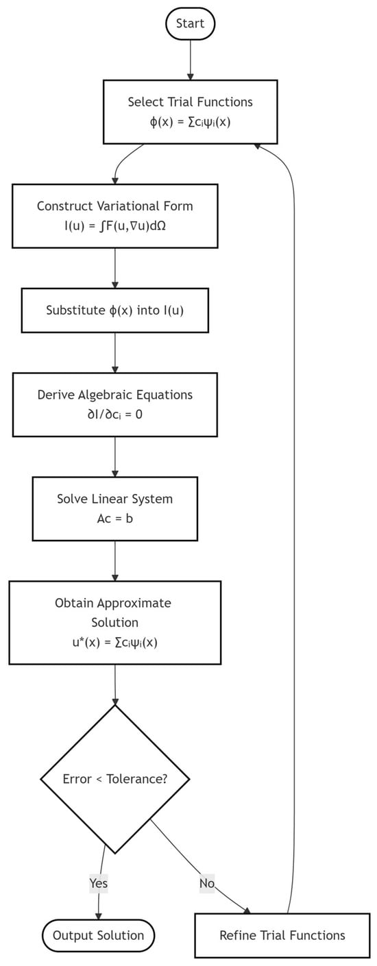
Figure 1. Generalized flowchart of the Ritz method implementation.

4. Case Study of Solving Seepage Problem by Ritz Method

In order to verify the effectiveness of Ritz’s method and analyze the accuracy of its approximate solutions with different orders, the following one-dimensional steady-state seepage problems is selected:

$${\displaystyle \frac{d^{2}p}{d{x}^2}}+Ap+Bx=0\hspace{1em}0<x<1$$

(25)

$$p=0,\hspace{1em}\mathrm{when}\hspace{1em}x=0 \mathrm{or} x=1$$

(26)

4.1. Potential Implementation Scenarios

Although the form of the equation is relatively simple, the terms of the equation can have a relatively broad physical meaning.

${\displaystyle \frac{d^{2}p}{d{x}^2}}$ is the second derivative of the pressure gradient, characterizing the seepage acceleration term. Within the framework of Darcy’s law, it corresponds to the diffusion term in the momentum conservation equation.

$Ap$ is a source/sink term related to pressure, which may represent ① the effect of rock compression (when $A$ > 0); ② the interaction between the fluid and porous medium (such as adsorption/desorption); ③ nonlinear seepage effects (such as threshold pressure gradient); and so on.

$Bx$ is an external force term related to position, which may describe ① gravitational differentiation (when B < 0); ② the pressure difference along the path due to injection and production (such as an injection well located at $x$ = 0 and a production well at $x$ = 1); and ③ an additional driving force caused by the heterogeneous permeability distribution.

Specifically, with different values of A and B, the above equation can represent various reservoir seepage scenarios. Research on new methods for solving it has certain practical significance.

4.1.1. Classic Darcy Flow (Linear Flow)

$$\mathrm{Parameter} \mathrm{conditions}: A=0 ,B=-{\displaystyle \frac{\mu q}{k{A}_c}}$$

$$\mathrm{The} \mathrm{form} \mathrm{of} \mathrm{the} \mathrm{equation}: {\displaystyle \frac{d^{2}p}{d^{2}x}}={\displaystyle \frac{\mu q}{k{A}_c}}x$$

where $k$ is the permeability, $q$ is the flow rate, $A_c$ is the cross-sectional area of corresponding flow, and $\mu$ is the dynamic viscosity. At this time, the equation can describe the pressure dissipation of single-phase fluid in homogeneous porous media or be applied to the productivity prediction of horizontal wells in conventional reservoirs, etc.

4.1.2. Nonlinear Flow in Low-Permeability Reservoirs (Threshold Pressure Gradient)

$$\mathrm{Parameter} \mathrm{conditions}: A={\displaystyle \frac{\beta }{k}}>0,B=-{\displaystyle \frac{\mu q}{k{A}_c}}$$

$$\mathrm{The} \mathrm{form} \mathrm{of} \mathrm{the} \mathrm{equation}: {\displaystyle \frac{d^{2}p}{d^{2}x}}+{\displaystyle \frac{\beta }{k}}p={\displaystyle \frac{\mu q}{k{A}_c}}x$$

where $\beta$ is the threshold pressure gradient. At this time, the equation can approximately reflect that fluids in low-permeability reservoirs need to overcome the threshold pressure to flow or explain phenomena such as “injection difficulty and production difficulty” in the waterflood development of low-permeability oilfields.

4.1.3. Matrix–Fracture Coupled Flow (Dual-Porosity Medium)

$$\mathrm{Parameter} \mathrm{conditions}: A=-{\displaystyle \frac{\alpha k_m}{k_f}}<0,B=0$$

$$\mathrm{The} \mathrm{form} \mathrm{of} \mathrm{the} \mathrm{equation}: {\displaystyle \frac{d^{2}p}{d^{2}x}}-{\displaystyle \frac{\alpha k_m}{k_f}}p=0$$

where $k_m$ is the permeability of the matrix, $k_f$ is the permeability of the fracture, and $\alpha$ is the fracture–matrix coupling coefficient. At this time, the equation can be approximately used to characterize the fluid exchange from fracture networks to the matrix in shale gas reservoirs or for simulating the linear flow stage of fractured horizontal wells.

4.1.4. Gravity-Driven Seepage Flow (Dipping Formation)

$$\mathrm{Parameter} \mathrm{conditions}: A=0,B=\rho g\sin \theta$$

$$\mathrm{The} \mathrm{form} \mathrm{of} \mathrm{the} \mathrm{equation}: {\displaystyle \frac{d^{2}p}{d^{2}x}}=-\rho g\sin \theta \cdot x$$

where $\theta$ is the formation dip angle. At this time, the equation can be approximately used for steam-assisted gravity drainage (SAGD) calculations in heavy oil reservoirs or for a simplified analysis of bottom water coning issues.

4.1.5. Chemical Adsorption/Desorption Effects (Unconventional Oil and Gas)

$$\mathrm{Parameter} \mathrm{conditions}: A=-{\displaystyle \frac{\lambda D_e}{k}}<0,B=0$$

$$\mathrm{The} \mathrm{form} \mathrm{of} \mathrm{the} \mathrm{equation}: {\displaystyle \frac{d^{2}p}{d^{2}x}}={\displaystyle \frac{\lambda D_e}{k}}p$$

At this time, the equation can be approximately used to explain the pressure oscillation during the desorption process of coalbed methane or to simulate the release of adsorbed gas in shale reservoirs.

4.2. Focused Analysis: Simplified Flow Scenarios with Constant A and B

In the following solution process of this formula, $A$ and $B$ can first be simply considered as constants, which can demonstrate and highlight the advantage of the Ritz method more clearly.

4.2.1. Exact Solution

According to the solving steps of the Ritz method discussed above, the equivalent variational form of the problem is

$$I={\displaystyle {\int }_0^1[{(\frac{dp}{dx})}^2-A{p}^2-2Bxp]dx}$$

(27)

According to the solution theory of ordinary differential equations, it is easy to know that the exact solution of this problem is

$$p(x)={\displaystyle \frac{B}{A}}[{\displaystyle \frac{\sin A^{1/2}x}{\sin A^{1/2}}}-x]$$

(28)

4.2.2. Trial Solution in Monomial Expression

The selected trial solution is

$${\tilde{p}}_1(x)=c_1{\varphi }_1(x)$$

(29)

In which

$${\varphi }_1(x)=x(1-x)$$

(30)

Obviously, the function satisfies the two boundary conditions shown in Equation (26). Substituting this trial solution into Equation (27) can obtain

$$I(c_1)={\displaystyle \frac{1}{3}}(1-{\displaystyle \frac{A}{10}})c_1{}^2-{\displaystyle \frac{B}{6}}{c}_1$$

(31)

Coefficient $c_1$ is determined according to Formula (24), which is

$${\displaystyle \frac{dI(c_1)}{d{c}_1}}={\displaystyle \frac{2}{3}}(1-{\displaystyle \frac{A}{10}})c_1-{\displaystyle \frac{B}{6}}=0$$

(32)

Therefore,

$$c_1={\displaystyle \frac{B}{4(1-A/10)}}$$

(33)

Finally, the monomial trial solution is obtained as follows:

$${\tilde{p}}_1(x)={\displaystyle \frac{B}{4(1-A/10)}}x(1-x)$$

(34)

4.2.3. Trial Solution in Binomial Expression

The selected trial solution is

$${\tilde{p}}_2(x)=c_1{\varphi }_1(x)+c_2{\varphi }_2(x)$$

(35)

In which

$${\varphi }_1(x)=x(1-x) \mathrm{and} {\varphi }_2(x)=x^2(1-x)$$

(36)

Obviously, both ${\varphi }_1(x)$ and ${\varphi }_2(x)$ satisfy the two boundary conditions shown in Equation (26). Substituting this trial solution into Equation (27) can obtain $I(c_1,c_2)$. Let

$${\displaystyle \frac{\mathsf{\partial }I(c_1,c_2)}{\mathsf{\partial }{c}_j}}=0\hspace{1em}\hspace{1em}j=1,2$$

(37)

Therefore, two algebraic equations about coefficients $c_1$ and $c_2$ can be obtained to determine the values of $c_1$ and $c_2$.

According to the above discussion on a binomial trial solution, it is not difficult to see that for the case of $A=B=1$, $c_1=71/369$, $c_2=7/41$, the binomial trial solution is

$${\tilde{p}}_2(x)=x(1-x)({\displaystyle \frac{71}{369}}+{\displaystyle \frac{7}{41}}x)$$

(38)

5. Discussion

5.1. Accuracy Analysis: Error Between Approximate and Exact Solutions

In order to compare with the exact solution and verify the accuracy of the Ritz approximate solution, it may be assumed that $A=1$, $B=1$ to investigate the difference between the monomial trial solution and the binomial trial solution and the exact solution.

Let the values of $x$ be 0.25, 0.50, 0.75, and 0.85, respectively, and calculate the pressure values of the exact solution and the Ritz monomial approximate solution at $x$ as Table 1 below:

Table 1. Exact solution and Ritz monomial approximate solution of pressure at different $x$ values when $A=B=1$.

$\mathit{x}$	0.25	0.5	0.75	0.85
Exact solution	0.04400	0.06974	0.06005	0.04282
Monomial approximate solution	0.0521	0.0694	0.0521	0.0354

These data are shown clearly in Figure 2 below to show the difference between the exact solution and the Ritz monomial approximate solution of pressure at different $x$ values when $A=B=1$.

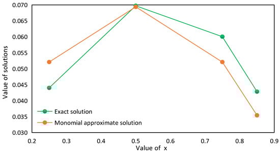
Figure 2. Exact solution and Ritz monomial approximate solution of pressure at different $x$ values when $A=B=1$.

Similarly, in order to compare the approximate solutions and verify the accuracy of the Ritz approximate solution, it may be assumed that $A=1$, $B=1$ to investigate the difference between the Ritz monomial trial solution and the binomial trial solution.

Let the values of $x$ be 0.25, 0.50, 0.75 and 0.85, respectively, and calculate the pressure values of the Ritz monomial approximate solution and binomial approximate solution at $x$ as Table 2 below:

Table 2. Ritz monomial and binomial approximate solution of pressure at different $x$ values when $A=B=1$.

$\mathit{x}$	0.25	0.5	0.75	0.85
Monomial approximate solution	0.0521	0.0694	0.0521	0.0354
Binomial approximate solution	0.04408	0.06944	0.06009	0.04302

These data are shown clearly in Figure 3 below to show the difference between the Ritz monomial and binomial approximate solution of pressure at different $x$ values when $A=B=1$.

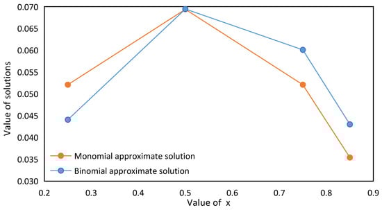
Figure 3. Ritz monomial and binomial approximate solution of pressure at different $x$ values when $A=B=1$.

Furthermore, in order to compare with the approximate solutions and verify the accuracy of the Ritz approximate solution, it may be assumed that $A=1$, $B=1$ to investigate the difference between the exact solution and the Ritz binomial trial solution.

Let the values of $x$ be 0.25, 0.50, 0.75, and 0.85, respectively, and calculate the pressure values of the exact solution and the Ritz binomial approximate solution at $x$ as Table 3 below:

Table 3. Exact solution and Ritz binomial approximate solution of pressure at different $x$ values when $A=B=1$.

$\mathit{x}$	0.25	0.5	0.75	0.85
Exact solution	0.04400	0.06974	0.06005	0.04282
Binomial approximate solution	0.04408	0.06944	0.06009	0.04302

These data are shown clearly in Figure 4 below to show the difference between the exact solution and the Ritz binomial approximate solution of pressure at different $x$ values when $A=B=1$.

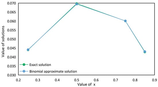
Figure 4. Exact solution and Ritz binomial approximate solution of pressure at different $x$ values when $A=B=1$.

To show the relative difference between the exact solution and approximate solution, “deviation percentage” was defined using the formula below:

$$Deviation percentage={\displaystyle \frac{Approximate solution-Exact solution}{Exact solution}}\times 100\%$$

(39)

Then the relative difference can be judged from the formula above.

These data are shown clearly in Figure 5 below to show the absolute value of the deviation percentage of the Ritz approximate solution from the exact solution of pressure at different $x$ values when $A=B=1$.

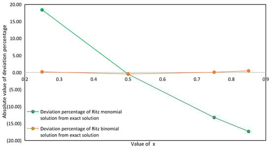
Figure 5. Deviation percentage of Ritz approximate solution from exact solution at different $x$ values when $A=B=1$.

According to the calculation results in Table 4 and the deviation between the approximate solution and the exact solution, we can see that the Ritz monomial approximate solution basically represents the numerical value of the exact solution, but it also shows a large deviation, the average range of deviation percentage is about ±15%, and the deviation is the smallest at $x=0.50$, which is only 0.48%. At the same time, it also shows that the deviation is not directly related to the coordinate position of the pressure point. Compared with the monomial approximate solution, the calculation accuracy of the binomial approximate solution is generally much higher. When $x=0.50$, the deviation between the monomial approximate solution and the binomial approximate solution is the closest, which is around 0.46%. Taken together, at different values of $x$, the deviation of the binomial approximate solution from the exact solution is only about 0.30% on average. The deviation is only 0.07% when 0.75 is taken. At the same time, it can be confirmed that the position where the deviation of the monomial approximate solution is the smallest is different from that of the binomial approximate solution, which further confirms that the deviation has nothing to do with the solution position of the pressure point.

Table 4. Deviation percentage of Ritz approximate solution from exact solution at different $x$ values when $A=B=1$.

$\mathit{x}$	0.25	0.5	0.75	0.85
Deviation percentage of Ritz monomial solution from exact solution (%)	18.41	−0.49	−13.24	−17.33
Deviation percentage of Ritz binomial solution from exact solution (%)	0.18	−0.43	0.07	0.47

5.2. Limitations of Ritz Method

The Ritz method, as a numerical approach based on variational principles, demonstrates unique advantages in solving seepage problems, such as rigorous theoretical foundations and systematic computational processes. However, it also has several significant limitations that require special attention in practical engineering applications.

First and foremost, the core issue of this method lies in its high dependence on the quality of trial function selection. When dealing with complex boundary conditions (e.g., irregular boundaries in heterogeneous reservoirs) or strongly nonlinear flow behaviors (e.g., seepage with slippage effects or stress sensitivity), constructing trial functions that both satisfy boundary conditions and accurately approximate the true solution becomes extremely challenging. This not only demands a deep understanding of the problem’s essence from researchers but also requires substantial experience in designing appropriate trial function forms. Secondly, the Ritz method faces severe computational efficiency challenges when handling high-dimensional or transient seepage problems. For three-dimensional seepage, the construction of trial functions and the corresponding integral calculations grow exponentially, leading to the so-called “curse of dimensionality.” For time-dependent transient seepage problems, the introduction of additional temporal variables further increases computational complexity. Moreover, since the method is fundamentally based on linear variational principles, it has inherent limitations in addressing strongly nonlinear seepage phenomena. For instance, threshold pressure gradient effects in low-permeability reservoirs or adsorption/desorption coupling processes in shale gas development are difficult to accurately describe using simple linear combinations of trial functions. Additionally, boundary condition treatment poses another major constraint for the Ritz method. In practical applications, it is often necessary to combine it with other methods (e.g., the Galerkin method) to relax the strict requirements on boundary conditions.

Nevertheless, this study provides new insights into solving oil and gas seepage problems. Future improvements may include developing adaptive trial function generation algorithms to reduce reliance on prior knowledge; incorporating machine learning techniques to optimize trial function selection; or coupling the Ritz method with other numerical methods (e.g., finite volume method, discrete element method) to leverage their respective strengths and expand its applicability to complex seepage problems. These enhancements will help overcome current limitations and enable the Ritz method to play a greater role in practical engineering applications such as oilfield development.

6. Conclusions

The study successfully applies the Ritz method to solve underground oil seepage problems, demonstrating its efficacy through variational theory and practical case analysis. Key findings include the following:

(1)

The Ritz method, as an integral approach, provides a viable solution for steady-state seepage problems in finite domains.

(2)

While the monomial approximate solution captures the general trend of the exact solution, it exhibits notable deviations (average ±15%).

(3)

The binomial approximate solution significantly improves accuracy, with deviations averaging only 0.30%, making it a reliable substitute for exact solutions.

(4)

The deviation between approximate and exact solutions is independent of the pressure point’s spatial position, underscoring the method’s robustness.

(5)

The Ritz method shows key limitations in oil–gas seepage problems: its accuracy heavily depends on trial function selection. For complex boundaries (such as strongly heterogeneous reservoirs) or nonlinear flows (with slippage/stress-sensitivity effect), constructing suitable trial functions becomes challenging. Three-dimensional transient problems will also face the “curse of dimensionality”, drastically reducing calculation efficiency. Current improvement measures can be considered, such as (1) combining with Galerkin’s method for better boundary handling; (2) using spectral methods for pressure field adaptation; and (3) coupling with numerical methods such as finite volume methods.

(6)

Although these suggested methods have demonstrated application potential in engineering problems such as multi-scale seepage in shale gas reservoirs and stress-coupled seepage in tight oil reservoirs, achieving an optimal balance between computational accuracy and efficiency remains a subject requiring in-depth research.

References

- Zhang, S.; Lv, Q.; Wang, J.; Liu, L.; Yu, C.; Ji, Y.; Wu, Y.; Hu, H.; Tao, D.; Zhang, M.; et al. Research and practice on deep development technology through flow field regulation in reservoirs with medium-high permeability and high water cut in Shengli Oilfield. Pet. Geol. Recovery Effic. 2025, 32, 88–101. [Google Scholar]
- Zhu, W.; Chen, Z.; Shang, X. Multiphysical field coupling in unconventional oil and gas reservoirs. Chin. J. Eng. 2023, 45, 1045–1056. [Google Scholar]
- Zhang, R.; Wang, T.; Wang, F.; Zhu, X.; Wang, Y.; Kou, S.; Wang, J. Time variation flow model of reservoir permeability based on effective cumulative water flux. Pet. Geol. Recovery Effic. 2025, 32, 162–173. [Google Scholar]
- Ning, W.; Xing, X.; Yang, Z.; Chen, R. The study of characteristics of the precipitated water of high water super heavy oil emulsion. Sci. Technol. Eng. 2015, 15, 177–180. [Google Scholar]
- He, D.; Ji, G.; Jiang, W.; Cheng, L.; Meng, D.; Wang, G.; Guo, Z.; Cheng, M.; Han, J. Differential development technological measures for high-water-cut tight sandstone gas reservoirs in western area of Sulige Gas Field. Nat. Gas Ind. 2022, 42, 73–82. [Google Scholar]
- Bao, J.; Li, L.; Ye, J.; Shi, J.; Zhang, J.; Zhu, H.; Jiang, N. Well location intelligent optimization method and its application for infill wells in high water cut complex fault-block oilfields. Acta Pet. Sin. 2017, 38, 444–452, 484. [Google Scholar]
- Sun, Z.; Li, X.; Xu, B.; Xiao, Z.; Zhang, Y.; Miao, Y.; Peng, Z.; Wang, X. Study on novel method of production capacity analysis on low permeability and unsaturated coal bed methane well. Coal Sci. Technol. 2019, 47, 238–243. [Google Scholar]
- Guo, J.; Li, J.; Yang, X.; Yang, J. Grey modeling based on productivity prediction of low permeability wells. Control Decis. 2019, 34, 2498–2504. [Google Scholar]
- Wu, Y. Percolation characteristics of low permeability carbonate heavy oil reservoir: A case study from O oilfield in Syria. Sci. Technol. Eng. 2017, 17, 159–162. [Google Scholar]
- Fu, N.; Tang, H.; Liu, Q. Technologies for fine adjustment in the middle-later development stage of low permeability tight sandstone gas reservoirs. J. Southwest Pet. Univ. (Sci. Technol. Ed.) 2018, 40, 136–145. [Google Scholar]
- Bian, X.; Zhang, S.; Zhang, J.; Wang, D. Well spacing design for low and ultra-low permeability reservoirs developed by hydraulic fracturing. Pet. Explor. Dev. 2015, 42, 646–651. [Google Scholar] [CrossRef]
- Zhao, M.; Fan, X. Optimized numerical simulation of the fracture network in the shale gas. Pet. Geol. Oilfield Dev. Daqing. 2019, 38, 167–174. [Google Scholar]
- Guo, X.; Yang, K.; Yang, Y.; Jia, H. Influence of seepage velocity on shale gas exploration by pore network simulation. J. Southwest Pet. Univ. (Sci. Technol. Ed.) 2019, 41, 19–27. [Google Scholar]
- Jin, X.; Li, G.; Meng, S.; Wang, X.; Liu, C.; Tao, J.; Liu, H. Microscale comprehensive evaluation of continental shale oil recoverability. Pet. Explor. Dev. 2021, 48, 222–232. [Google Scholar] [CrossRef]
- Xu, R.; Guo, T.; Qu, Z.; Chen, M.; Qin, J.; Mou, S.; Chen, H.; Zhang, Y. Numerical simulation of fractured imbibition in a shale oil reservoir based on the discrete fracture model. Chin. J. Eng. 2022, 44, 451–463. [Google Scholar]
- Mao, X.; Hu, G.; Zhang, X.; Zhang, W.; Qin, Y.; Wang, C. Simulation method of oil-water two-phase transient flow in dual-porosity system in tight reservoir. J. Shenzhen Univ. (Sci. Eng.) 2021, 38, 572–578. [Google Scholar] [CrossRef]
- Li, Q.; Wu, J.; Li, Q.; Wang, F.; Cheng, Y. Sediment Instability Caused by Gas Production from Hydrate-Bearing Sediment in Northern South China Sea by Horizontal Wellbore: Sensitivity Analysis. Nat. Resour. Res. 2025, 34, 1667–1699. [Google Scholar]
- Li, Q.; Li, Q.; Wu, J.; Li, X.; Li, H.; Cheng, Y. Wellhead Stability During Development Process of Hydrate Reservoir in the Northern South China Sea: Evolution and Mechanism. Processes 2025, 13, 40. [Google Scholar] [CrossRef]
- Yin, J.; Yang, F.; Wu, M.; Liu, X. Non-Boltzmann porous medium flow movement law based on homotopy perturbation method. Water Resour. Power 2016, 34, 70, 136–138. [Google Scholar]
- Shao, W.; Li, J. An absorbing boundary condition based on the perfectly matched layer technique in discontinuous Galerkin Boltzmann Method. J. Eng. Thermophys. 2019, 40, 767–775. [Google Scholar]
- Zhao, Z. Thermodynamic analysis for the gas production from gas hydrate by heating. China Min. Mag. 2013, 8, 125–128. [Google Scholar]
- Zhang, J.; Li, C.; Zhang, X.; Li, Z. Laplace transform method of discrete data in well test analysis. Nat. Gas Ind. 2004, 24, 100–102. [Google Scholar]
- Liu, H.; Wang, X.; Zhang, F.; Niu, X. Laplace transform finite difference method for well-test problem with one-dimensional seepage flow. Chin. J. Comput. Phys. 2012, 29, 245–249. [Google Scholar]
- Liang, N.; Qi, C. A new dynamic semi-analytical algorithm of structural system—Laplace integral transform method of dynamic analysis of underground structures. Rock Soil Mech. 2010, 31, 198–206. [Google Scholar]
- Zeng, Y.; Wang, B.; Nie, R. The porous flow model of multi-stage fractured horizontal well in linear composite oil reservoirs. Acta Pet. Sin. 2017, 38, 687–695, 720. [Google Scholar]
- Huo, J.; Jia, Y.; Jiang, W. DST slug well test for low velocity non-Darcy flow in dual-permeability reservoirs. Pet. Explor. Dev. 2005, 32, 98–100. [Google Scholar]
- Tang, X.; Hu, W.; Yan, L.; Zheng, J. Modeling of reservoir dynamic performance by TEM method. Geophys. Prospect. Pet. 2004, 43, 192–195. [Google Scholar]
- Meng, X.; Du, Z.; Wang, X.; Bai, Y.; Shao, C. Seepage characteristics and their affecting factors for the fractured horizontal cracks. Pet. Geol. Oilfield Dev. Daqing 2016, 35, 73–77. [Google Scholar]
- Shen, Y. Integral Equation, 3rd ed.; Tsinghua University Press: Beijing, China, 2012. [Google Scholar]
- Shi, Z. Variational Principle and Finite Element Method; National Defense Industry Press: Beijing, China, 2016. [Google Scholar]
- Kong, X. Advanced Flow in Porous Media; Press of China University of Science and Technology: Hefei, China, 2010. [Google Scholar]
- Song, S.; Zhang, G. Theory and Application of Variational Method, 2nd ed.; Science Press: Beijing, China, 2019. [Google Scholar]
- Wu, C. Methods of Mathematical Physics, 4th ed.; Higher Education Press: Beijing, China, 2010. [Google Scholar]
- Lao, D. Fundamentals of the Calculus of Variations, 3rd ed.; National Defense Industry Press: Beijing, China, 2015. [Google Scholar]
Disclaimer/Publisher’s Note: The statements, opinions and data contained in all publications are solely those of the individual author(s) and contributor(s) and not of MDPI and/or the editor(s). MDPI and/or the editor(s) disclaim responsibility for any injury to people or property resulting from any ideas, methods, instructions or products referred to in the content. |
© 2025 by the authors. Licensee MDPI, Basel, Switzerland. This article is an open access article distributed under the terms and conditions of the Creative Commons Attribution (CC BY) license (https://creativecommons.org/licenses/by/4.0/).