A Multi-Vector Modulated Model Predictive Control Based on Coordinated Control Strategy of a Photovoltaic-Storage Three-Port DC–DC Converter ^†

Abstract

As a core component of the photovoltaic-storage microgrid systems, three-port DC–DC converters have attracted significant attention in recent years. This paper proposes a multi-vector modulated model predictive control (MVM-MPC) method based on vector analysis for a non-isolated three-port DC–DC converter formed by paralleling two bidirectional DC–DC converters. The proposed modulated MPC method utilizes three basic vectors to calculate the optimal switching sequence for minimizing the error vector. It can significantly minimize voltage ripple while maintaining the nonlinear and dynamic performance characteristics of a traditional MPC. MATLAB/Simulink R2024a simulations and hardware-in-loop (HIL) experimental results demonstrate that, compared with finite control set MPC and traditional two-vector modulated MPC methods, the proposed approach achieves remarkable reductions in current ripple and voltage ripple, along with excellent dynamic performance featuring smooth mode-switching.

1. Introduction

With the development of global economy, energy shortages and environmental pollution have become prominent issues. As a major carbon-emitting sector, the power industry urgently needs to transform towards a green and low-carbon model. Photovoltaic power generation has become the mainstay of renewable energy due to its advantages such as flexible deployment, short construction period, and proximity to load centers. From 2020 to 2024, the global cumulative installed capacity of photovoltaic power jumped from 127 GW to 592 GW, an increase of 465 GW over four years, with particularly significant growth from 2022 to 2023, marking that photovoltaic power has entered an accelerated phase of popularization. In 2024, the newly added global energy storage capacity was 79.2 GW/188.5 GWh, marking a year-on-year increase of 82.1%. The total demand is expected to reach 828 GWh by 2030. The coordination of photovoltaic power and energy storage has become a key method to reduce carbon emissions and energy waste [1,2].

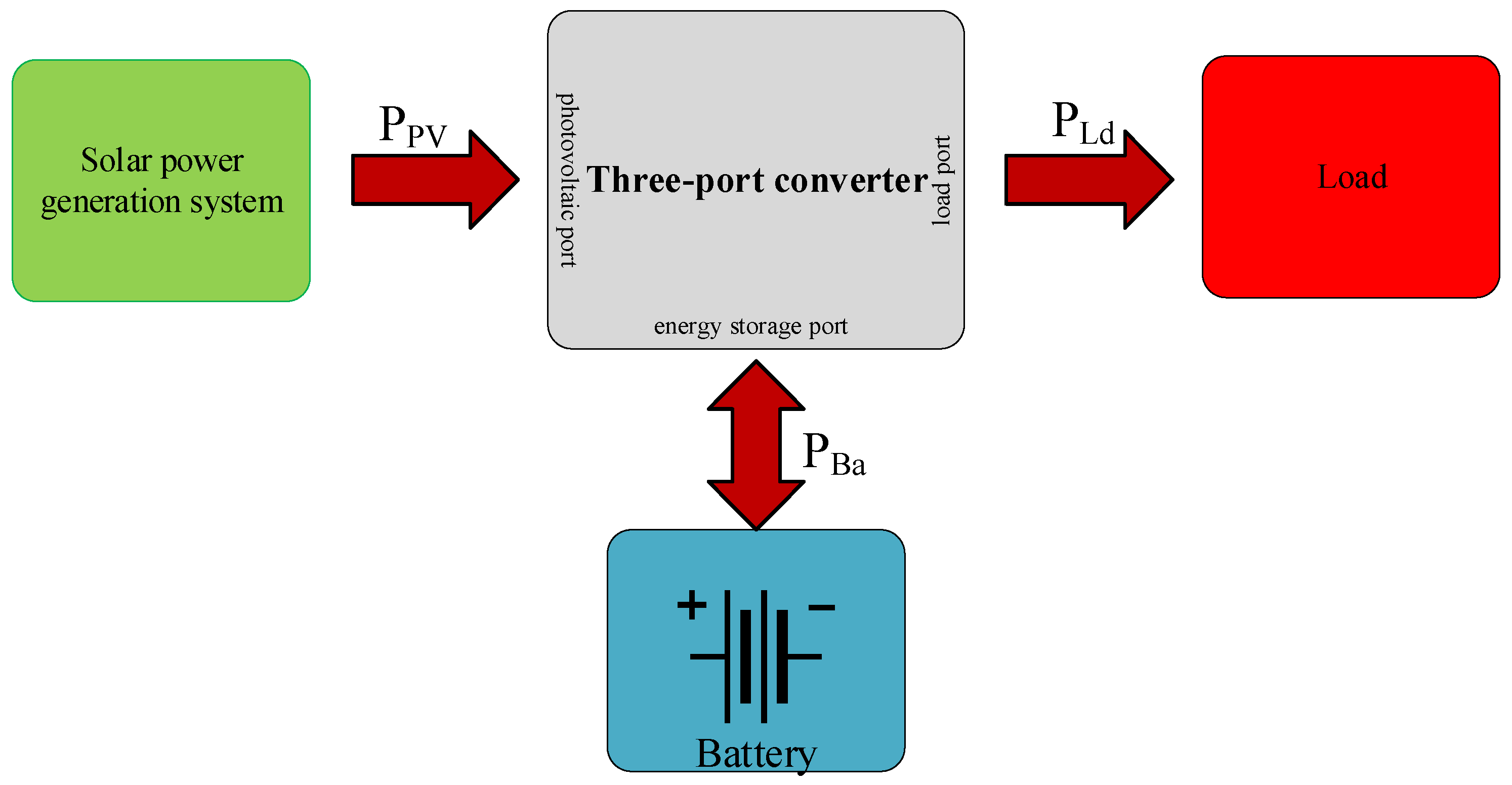
As a core component of the photovoltaic-storage microgrid systems, three-port converters can effectively integrate photovoltaic sources, energy storage units, and loads, enabling flexible power flow management to enhance photovoltaic energy utilization efficiency and regional system stability [3]. As shown in Figure 1, the three-port photovoltaic-storage converter comprises three ports: a photovoltaic port, a battery port, and a load port. Depending on solar irradiance and load demand, it operates in distinct working modes [4,5]. Dual-Input Single-Output (DISO) mode: when solar irradiance weakens and photovoltaic output becomes insufficient, the energy storage unit discharges to complement the photovoltaic array, jointly supplying power to the load and ensuring its normal operation. Single-Input Dual-Output (SIDO) mode: when solar irradiance is sufficient, the photovoltaic array generates power exceeding the actual load demand. In this mode, the energy storage unit stores surplus energy while the photovoltaic array simultaneously supplies power to the load, achieving maximum energy utilization.

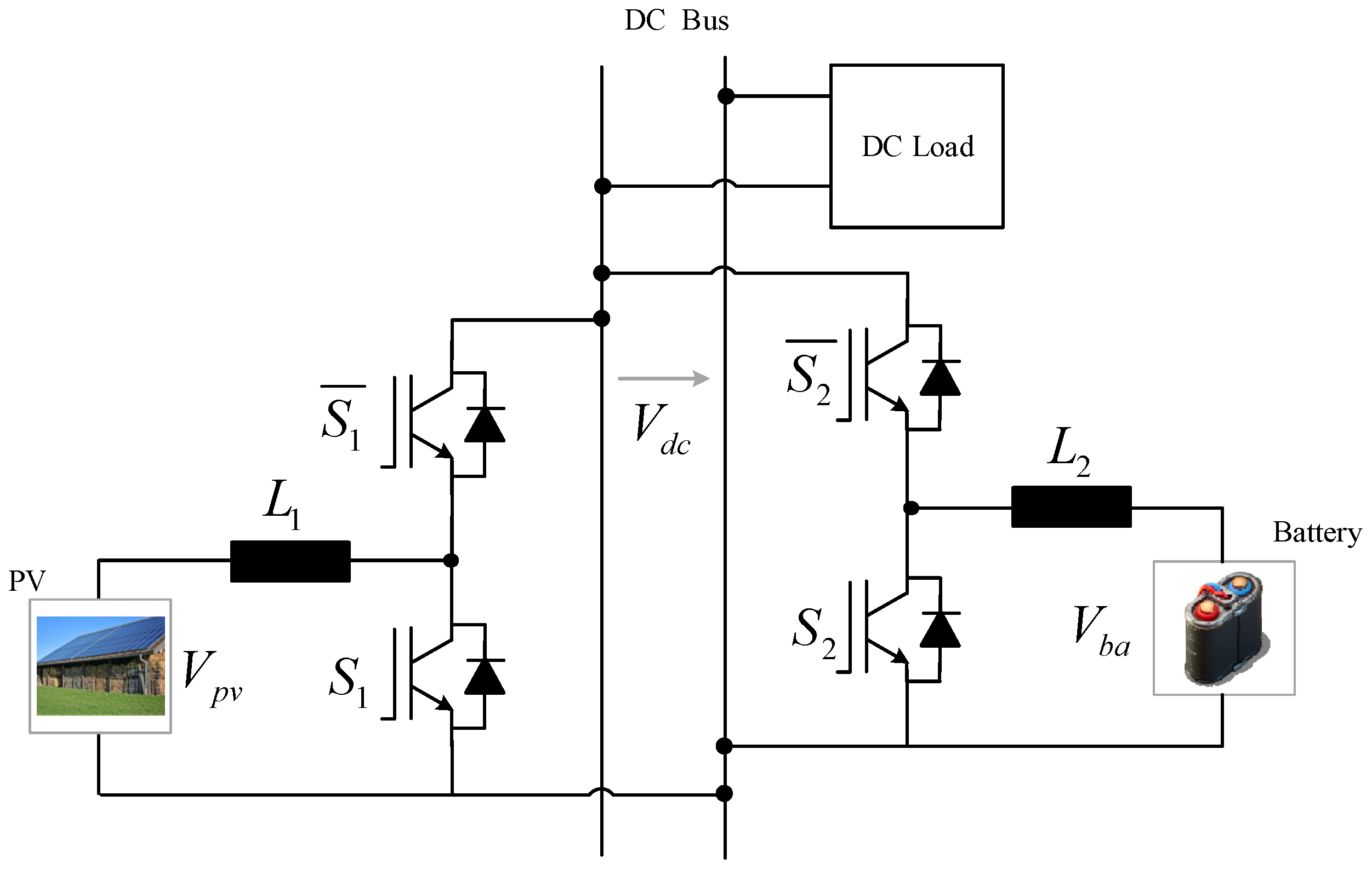
The mainstream system configuration of photovoltaic-storage three-port DC–DC converters is illustrated in Figure 2 [6,7,8,9,10]. This system integrates the load, photovoltaic (PV) array, and battery through two parallel bidirectional synchronous rectification DC–DC converter circuits, enabling power transmission in any direction as required. Currently, these two DC–DC converters are predominantly controlled independently. For instance, the PV-side DC–DC converter adopts maximum power point tracking (MPPT) control strategies, such as the Perturb and Observe (P&O) method, to regulate the duty cycle of switching devices, ensuring the PV panel operates at its maximum power point and improving energy conversion efficiency [11,12,13]. In essence, MPPT achieves this by adjusting the input inductor current. The battery-side bidirectional DC–DC converter typically employs dual-loop control—an outer voltage loop used to stabilize the DC bus voltage, and an inner current loop used to regulate the charging/discharging current. For example, the outer voltage loop may use proportional–integral (PI) control or advanced active disturbance rejection control (ADRC), while the inner current loop may utilize PI control or MPC [14,15]. When the DC bus voltage is low, the battery discharges (Boost mode); when the voltage is high, the battery charges (Buck mode). However, the parallel operation of the two bidirectional DC–DC converters (PV-side and battery-side) through the DC bus introduces a mutual coupling mechanism. This mechanism exerts influence on bus voltage stability, power supply quality, and smooth mode-switching control. Therefore, it is imperative to explore novel control strategies to coordinate the operation of these two converters, thereby minimizing the adverse effects of the coupling mechanism.

Model predictive control (MPC), as an advanced control strategy, has demonstrated broad application prospects in various fields due to its predictive capability, multi-variable handling, and constrained optimization advantages. For the two parallel bidirectional DC–DC converter circuits (non-isolated topology with four switches), studies in [16,17] proposed a finite control set MPC (FCS-MPC) with the objective of minimizing the cost function (considering the power tracking error), where only one switching state (corresponding to a single vector) is selected to minimize the cost function. However, this approach suffers from variable switching frequencies and tracking errors due to the inability of a single vector to cover all possible reference vector directions. To address these issues, Ref. [18] proposed a multi-mode partitioning method combined with MPC, which predicts duty cycles under different modes to select the optimal mode and incorporates a hysteresis mechanism to avoid frequent switching. However, this method requires additional hysteresis logic for mode transitions and fixes duty cycles in intermediate modes, which limits flexibility. By designing an adaptive cost function, smooth switching between Buck mode, Boost mode, and critical mode is achieved, while avoiding complex parameter tuning processes [19]. However, the control performance highly depends on the accuracy and sampling frequency of voltage and current sensors. If there is noise or delay in sampling, it may lead to the accumulation of prediction errors and affect the control effect. Moreover, it is necessary to design additional digital filtering algorithms, increasing software complexity. In [20], a modulated model predictive control (MMPC) method was developed based on vector analysis, and a comprehensive simulation comparison has not been discussed.

Building on these foundations, this paper proposes a modulated model predictive control strategy for three-port converters. The approach involves the following:

(1)

Deriving inductor current increments from the system’s discrete-time mathematical model.

(2)

Establishing a four basic vector coordinate system and reference vector.

(3)

Calculating optimal duty cycles using three basic vectors and adopting adaptive strategies to minimize the error vector based on the reference vector’s position.

(4)

Generating fixed-frequency switching sequences via a PWM module after determining duty cycles.

Compared with traditional MPCs, the proposed modulated MPC offers fixed-frequency switching through vector synthesis, enabling continuous control, error-free tracking of reference vectors within the four basic vector coordinate system, significant reductions in current/voltage ripple, and enhanced dynamic performance.

2. Operating Principles of Three-Port DC–DC Converters

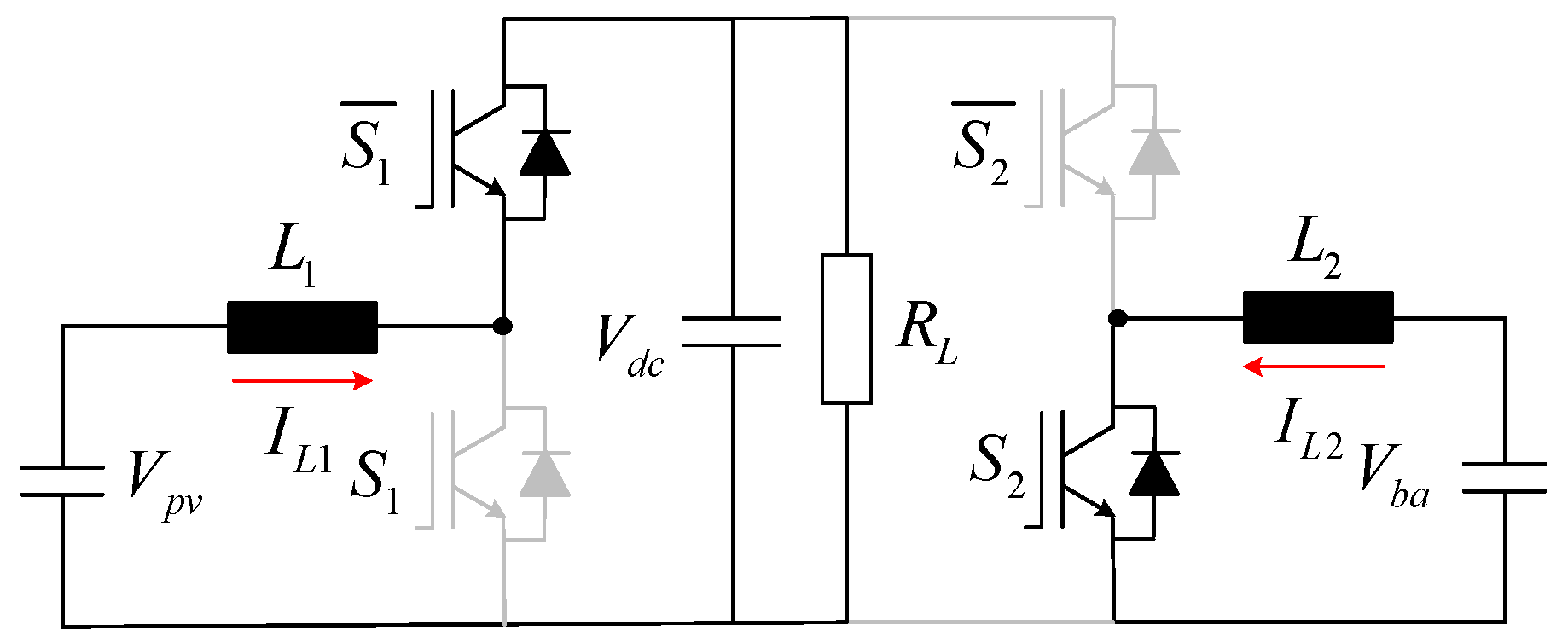
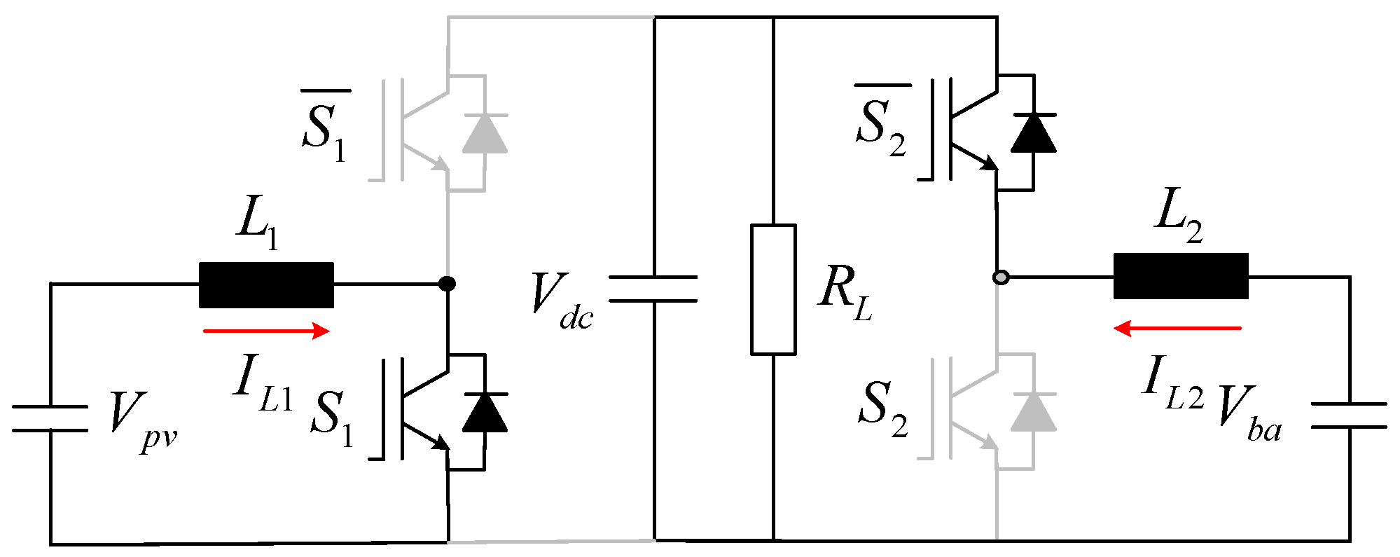
To optimize the design of control strategies and achieve smooth mode transitions, this section analyzes and models the operational states of the topology. A simplified diagram of the three-port DC–DC converter is shown in Figure 3. The converter employs two complementary power switching devices, resulting in four distinct operating modes.

Mode I: Switches S₁ and S₂ are both turned off (i.e., S₁ = 0 and S₂ = 0). The corresponding circuit diagram and current flow are illustrated in Figure 4 below. The governing equations in the continuous time domain are derived as follows:

$$\mathrm{I}:\left\{\begin{array}{l}{L}_1{\displaystyle \frac{d{I}_{L1}}{dt}}=V_{pv}-V_{dc}\hfill \\ L_2{\displaystyle \frac{d{I}_{L2}}{dt}}=V_{ba}-V_{dc}\hfill \end{array}\right.$$

(1)

Mode II: Switches S₁ is turned of and S₂ is turned on (i.e., S₁ = 0 and S₂ = 1). The corresponding circuit diagram and current flow are illustrated in Figure 5 below. The governing equations in the continuous time domain are derived as follows:

$$\mathrm{II}:\left\{\begin{array}{l}{L}_1{\displaystyle \frac{d{I}_{L1}}{dt}}=V_{pv}-V_{dc}\hfill \\ L_2{\displaystyle \frac{d{I}_{L2}}{dt}}=V_{ba}\hfill \end{array}\right.$$

(2)

Mode III: Switches S₁ is turned on and S₂ is turned off (i.e., S₁ = 1 and S₂ = 0). The corresponding circuit diagram and current flow are illustrated in Figure 6 below. The governing equations in the continuous time domain are derived as follows:

$$\mathrm{III}:\left\{\begin{array}{l}{L}_1{\displaystyle \frac{d{I}_{L1}}{dt}}=V_{pv}\hfill \\ L_2{\displaystyle \frac{d{I}_{L2}}{dt}}=V_{ba}-V_{dc}\hfill \end{array}\right.$$

(3)

Mode IV: Switches S₁ and S₂ are both turned on (i.e., S₁ = 1 and S₂ = 1). The corresponding circuit diagram and current flow are illustrated in Figure 7 below. The governing equations in the continuous time domain are derived as follows:

$$\mathrm{IV}:\left\{\begin{array}{l}{L}_1{\displaystyle \frac{d{I}_{L1}}{dt}}=V_{pv}\hfill \\ L_2{\displaystyle \frac{d{I}_{L2}}{dt}}=V_{ba}\hfill \end{array}\right.$$

(4)

To model the converter’s behavior, the switching function S_i is defined as (i = 1, 2) = 1, with S_i being represented as ON and vice versa. By combining the four operational mode equations using logical operators (e.g., XOR for mutually exclusive states), a unified expression is derived. Applying the forward difference approximation for derivative discretization, the following discrete time state–space model is obtained:

$$\left\{\begin{array}{l}{I}_{L1}^{k+1}={\displaystyle \frac{(V_{pv}^k-(1-S_1)V_{dc}^k)T}{L_1}}+I_{L1}^k\\ I_{L2}^{k+1}={\displaystyle \frac{(V_{dc}^k-(1-S_2)V_{ba}^k)T}{L_2}}+I_{L2}^k\end{array}\right.$$

(5)

where $T$ stands for the sampling period, and $V_{pv}^k$, $V_{dc}^k$, and $V_{ba}^k$ represent the sample values at time k for PV voltage, DC bus voltage, and battery voltage. $I_{L1}^k$ and $I_{L2}^k$ represent the sample values at time k for the PV inductor current, and battery inductor current, respectively. $I_{L1}^{k+1}$ and $I_{L2}^{k+1}$ are the prediction values at the time (k + 1) for those two currents, respectively. Notably, Equation (5) indicates that the system states at the time (k + 1) can be predicted by a mathematical model with the system state at time k.

3. Multi-Vector Modulated Model Predictive Control (MMPC) for Three-Port DC–DC Converters

FCS-MPC’s function is to predict the future behavior of the system and to select the optimal control action by traversing a finite number of switch state combinations. The control variables (such as the on/off states of switching tubes) are restricted to a finite number of discrete combinations. The specific control process is as follows:

(1)

System Modeling

Establish a discretized mathematical model of the controlled object for predicting future states. The following is a typical model form:

$$x\left(k+1\right)=f\left(x\left(k\right), u\left(k\right)\right)$$

(6)

where x(k) represents the current state (such as inductor current and capacitor voltage), and u(k) denotes the control input (switch state combination). The discretized mathematical model of the finite-set MPC for the topology in Section 2 is as follows:

$$\left\{\begin{array}{l}{I}_{L1}^{k+1}={\displaystyle \frac{(V_{pv}^k-(1-S_1)V_{dc}^k)T}{L_1}}+I_{L1}^k\\ I_{L2}^{k+1}={\displaystyle \frac{(V_{dc}^k-(1-S_2)V_{ba}^k)T}{L_2}}+I_{L2}^k\end{array}\right.$$

(7)

(2)

State Prediction

Traverse all possible switch combinations, such as 8 switch combinations (2³) for a three-phase inverter, and 4 combinations (2²) for the dual-switch system of the photovoltaic energy storage three-port DC/DC converter in Section 2, to predict the system state at the next moment. For each candidate switch state ui, calculate the predicted value x(k + 1).

(3)

Cost Function Evaluation

Design a cost function to quantify the control objectives. The following is a common form:

$$J={\displaystyle \sum _{i=1}^N(\Vert }{x}_{ref}-x(k+i){\Vert }^2+\lambda \Vert u(k+i-1){\Vert }^2)$$

(8)

where the first part of the function is the tracking error term (such as current/voltage tracking error), the second part is the constraint term (such as switch switching frequency suppression, voltage/current limiting), and is the weighting factor used to adjust the priority of different objectives. The cost function of the finite-set MPC for the topology in Section 2 is as follows:

$$J={\gamma }_{I_{L1}}{(I_{L{1}_{ref}}-I_{L{1}_{next}})}^2+{\gamma }_{I_{L2}}{(I_{L{2}_{ref}}-I_{L{2}_{next}})}^2+{\gamma }_{sw}({(pre{v}_{S1}-S_1)}^2+{(pre{v}_{S2}-S_2)}^2)$$

(9)

(4)

Optimal Decision-Making

Select the switch state that minimizes the cost function as the following current control input:

$$u^{*}(k)=\arg \min J$$

(10)

(5)

Control Implementation

Apply the optimal switch state $u^{\mathrm{*}}\left(k\right)$ directly to the system without the need for PWM modulation.

FSC-MPC focuses on discrete switch states. For example, switching devices in power electronics have only a finite number of possible combinations. Traditional modulated MPC usually deals with continuous control inputs, such as duty cycle or voltage, and finds the optimal control sequence by solving an optimization problem.

Therefore, the discretized mathematical model of traditional modulated MPC for the topology in Section 2 is as follows:

$$\left\{\begin{array}{l}{I}_{L1}^{k+1}={\displaystyle \frac{(V_{pv}^k-(1-D_{S1})V_{dc}^k)T}{L_1}}+I_{L1}^k\\ I_{L2}^{k+1}={\displaystyle \frac{(V_{dc}^k-(1-D_{S2})V_{ba}^k)T}{L_2}}+I_{L2}^k\end{array}\right.$$

(11)

Then, the main difference in the second-step state prediction is that traditional modulated MPC loops through D_S1 and D_S2, for example, searching for the optimal duty cycle from 0 to 1 with a step size of 0.1. For a dual-switch system, there are 100 combinations. Then, the PWM modulation is carried out.

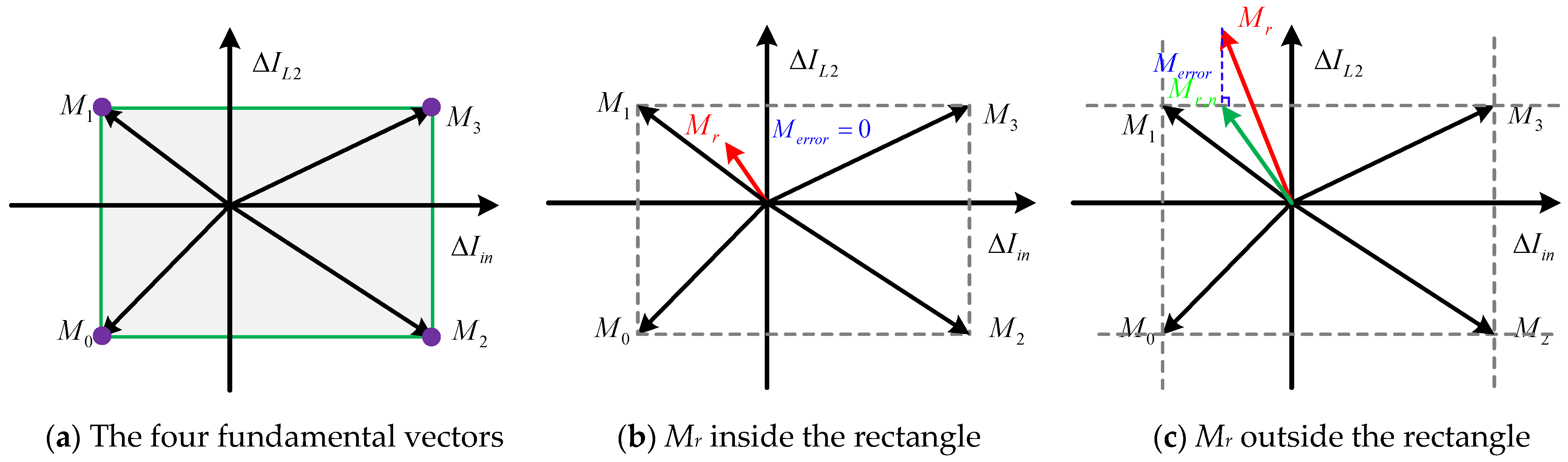
FSC-MPC only selects one switch state, which cannot fully track the reference value, leading to large current and voltage ripples. Meanwhile, the variable switching frequency increases the complexity of filter design. The conventional FCS-MPC only uses one fundamental vector to calculate the duty cycle; thus, only the four points (purple points in Figure 2) can achieve error-free regulation. The TM-MPC uses two fundamental vectors to calculate the duty cycle; thus, only with the reference vector being on the boundary enclosed by the four fundamental vectors (green line in Figure 2) can error-free regulation be achieved.

To address these challenges, this paper proposes a multi-vector modulated MPC strategy. By synthesizing three basic vectors to coordinate and compute the optimal switching sequence, the method minimizes voltage ripple and achieves error-free tracking of reference values. The detailed control approach is shown below.

Based on Equation (5), the inductor current increment over one sampling period is derived as follows:

$$\left\{\begin{array}{l}\Delta I_{L1}^{k+1}=I_{L1}^{k+1}-I_{L1}^k={\displaystyle \frac{(V_{pv}^k-(1-S_1)V_{dc}^k)T}{L_1}}\\ \Delta I_{L2}^{k+1}=I_{L2}^{k+1}-I_{L2}^k={\displaystyle \frac{(V_{ba}^k-(1-S_2)V_{dc}^k)T}{L_2}}\end{array}\right.$$

(12)

The increment value under four different operation modes is summarized in

Table 1. The current increment values under different operation modes.

Operation State	$\mathit{\Delta }{\mathit{I}}_{\mathit{L}1}$	$\mathit{\Delta }{\mathit{I}}_{\mathit{L}2}$	Quadrant
M0: State I	$M_{0,x}:(V_{pv}-V_{dc})T/L_1$	$M_{0,\mathrm{y}}:(V_{\mathrm{ba}}-V_{dc})T/L_2$	Third
M1: State II	$M_{1,x}:(V_{pv}-V_{dc})T/L_1$	$M_{1,y}:V_{ba}T/L_2$	Second
M2: State III	$M_{2,x}:V_{pv}T/L_1$	$M_{2,\mathrm{y}}:(V_{\mathrm{ba}}-V_{dc})T/L_2$	Fourth
M3: State IV	$M_{3,x}:V_{pv}T/L_1$	$M_{3,y}:V_{ba}T/L_2$	First

, and a vector coordinate system based on the increments is established. Here, the x-axis stands for the input inductor current increments, and the y-axis stands for the output inductor current increments. Benefiting from the symmetrical structure, we can obtain four symmetric fundamental vectors based on different operation modes, which can form a rectangle modulation region as shown in Figure 8a. Meanwhile, we can obtain the reference vector as follows:

$$M_r(\Delta I_{L1}^r,\Delta I_{L2}^r)=M_r\left({\displaystyle \frac{I_{L1}^{*}-I_{L1}^k}{M_{r,x}}},{\displaystyle \frac{I_{L2}^{*}-I_{L2}^k}{M_{r,y}}}\right)$$

(13)

The conventional MPC directly calculates the desired switching states with a cost function in each sampling cycle, which cannot realize error-free tracking because only one fundamental vector is used. In this paper, three fundamental vectors are used to calculate the optimal switching sequence to minimize the error vector. If we choose the three fundamental vectors M_i, M_j, and M_l with a duty cycle of d_i, d_j, and d_l (d_i + d_j + d_l = 1) we obtain the following:

$$\begin{array}{c}{M}_s=d_i{M}_i+d_j{M}_j+(1-d_i-d_j)M_l\\ (i=0,1,2,3;j=0,1,2,3;l=0,1,2,3;i\ne j\ne l)\end{array}$$

(14)

Possible synthetic vectors will form a rectangle, as shown in the dotted box of Figure 8b. In this situation, the error vector M_error can approach zero when M_r is inside the rectangle, resulting in a theoretical control error near zero.

$$M_{error}=\min \left|M_s-M_r\right|=0, M_r \mathrm{is} \mathrm{inside} \mathrm{the} \mathrm{rectangle}$$

(15)

When the reference vector M_r is outside the rectangle, the error vector cannot approach the error-free zone even with three fundamental vectors. In this situation, we can make a line perpendicular to the nearest edge of the rectangle, shown in Figure 8c, and then obtain a new reference vector M_r,n that can be modulated with three fundamental vectors to minimize the error vector. Fortunately, we can easily obtain the nearest vector by the region of the reference vector due to the symmetric of the fundamental vectors, which can be expressed as follows:

$$M_{r,n}\left(\begin{array}{l}{M}_{r,x}=\left\{\begin{array}{l}{M}_{1,x} \mathrm{if}(M_{r,x}<M_{1,x})\\ M_{r,x} \mathrm{if}(M_{1,x}\le M_{r,x}\le M_{3,x})\\ M_{3,x} \mathrm{if}(M_{3,x}<M_{r,x})\end{array}\right. , \\ M_{r,y}=\left\{\begin{array}{l}{M}_{0,y} \mathrm{if}(M_{r,y}<M_{0,y})\\ M_{r,y} \mathrm{if}(M_{0,y}\le M_{r,y}\le M_{1,y})\\ M_{1,y} \mathrm{if}(M_{1,y}<M_{r,y})\end{array}\right.\end{array}\right)$$

(16)

After we obtain the reference vector, we can choose the two group vectors G1 (M₀, M₁, M₂) and G1 (M₁, M₂, M₃) to obtain the optimal switching sequences, which can fully cover the entire modulation area. The detailed formula for G1 and G2 can be expressed as:

$$\begin{array}{l}\mathrm{G}1:\left\{\begin{array}{l}{M}_r=d_0{M}_0+d_1{M}_1+(1-d_1-d_0)M_2\\ d_3=0 \\ 0\le d_0\le 1\\ 0\le d_1\le 1\\ 0\le 1-d_1-d_0\le 1\end{array}\right.\\ \mathrm{G}2: \left\{\begin{array}{l}{M}_r=d_1{M}_1+d_2{M}_2+(1-d_1-d_2)M_3\\ d_0=0 \\ 0\le d_1\le 1\\ 0\le d_2\le 1\\ 0\le 1-d_1-d_2\le 1\end{array}\right. \end{array}$$

(17)

Theoretically, we should locate where M_r to determine which groups will be chosen. However, the optimal duty cycle can be calculated, which satisfies all constraints in Equation (11). After calculating the duty cycle for each vector, the duty cycle for S1 and S2 can be obtained as follows:

$$\left\{\begin{array}{l}{D}_1=d_2 +d_3\\ D_2=d_1 +d_3\end{array}\right.$$

(18)

where D₁ is the duty cycle for S₁, and D₂ is the duty cycle for S₂. Then, the PWM module is used to generate an optimal sequence, obtaining fixed switching benefits. The overall control strategy and the flowchart of the proposed MVM-MPC are shown in Figure 9.

4. Simulation Validation

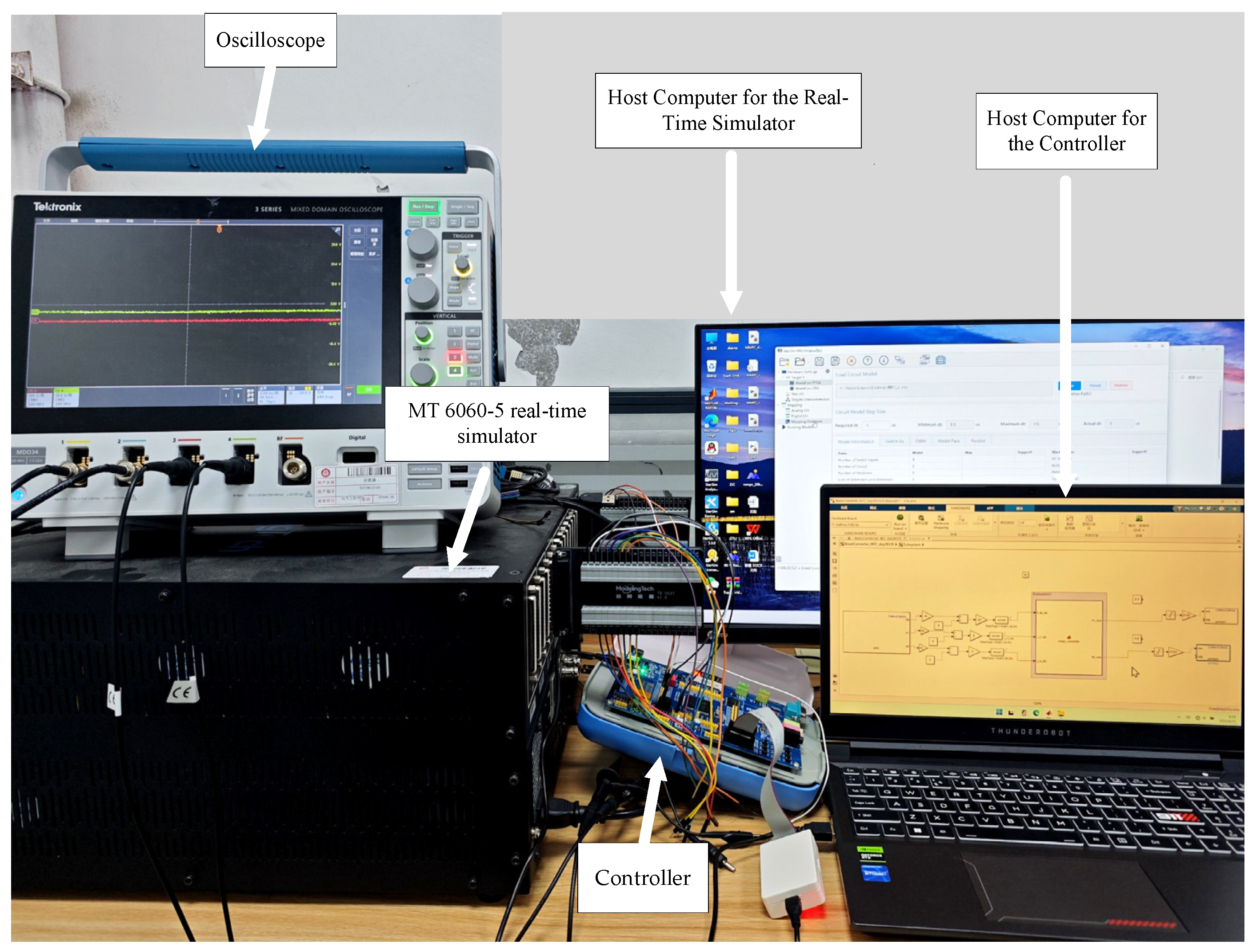
To validate the proposed control strategy, a simulation platform was developed using the MATLAB/Simulink 2024a, with detailed design parameters summarized in

Table 2. Design parameters.

Parameters	Value	Parameters	Value
Battery voltage	12 V DC	Calculation Frequency	20 kHz
PV Voltage	24 V DC	DC bus Voltage	30 V
Inductors L1/L2	500 μH	DC bus Capacitor	1000 μF

. The simulation was conducted under two operational modes based on the relationship between the photovoltaic port input power and the DC load conditions.

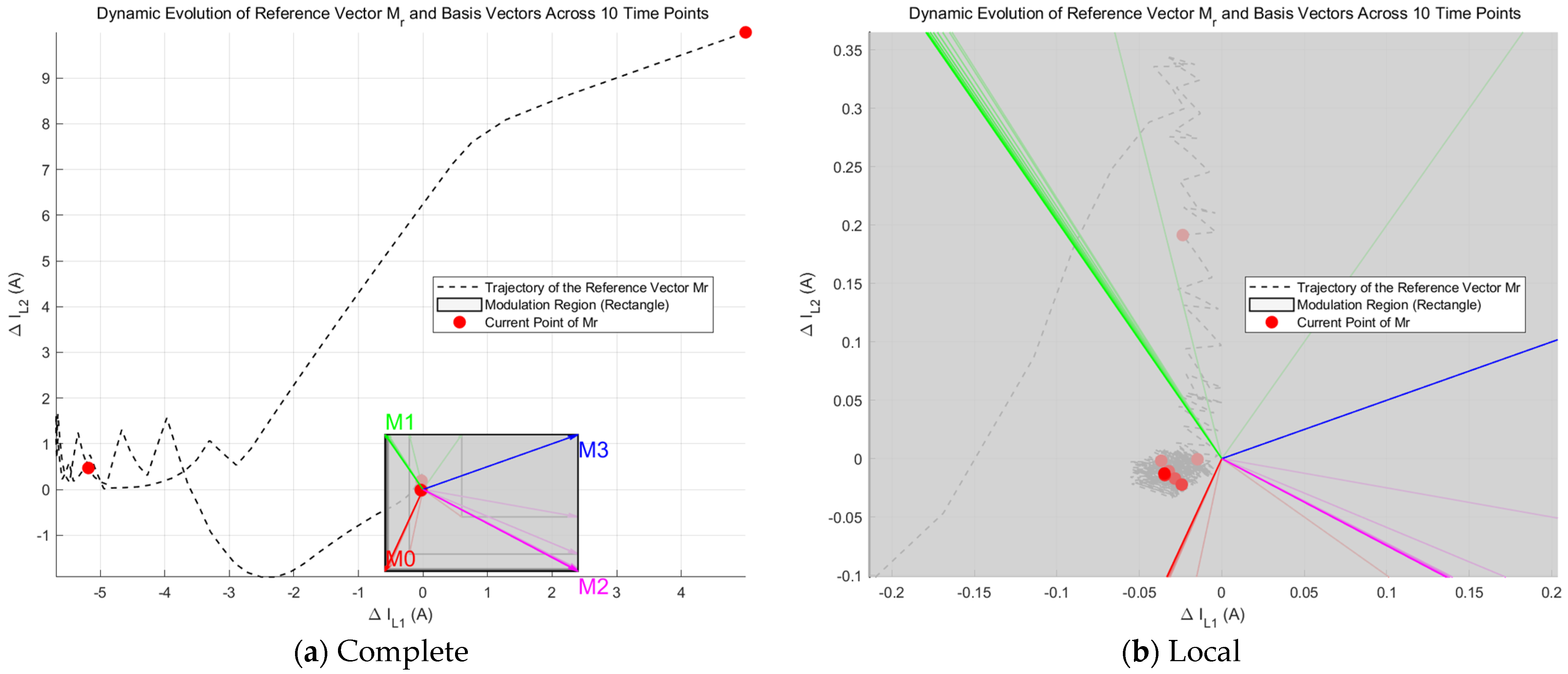
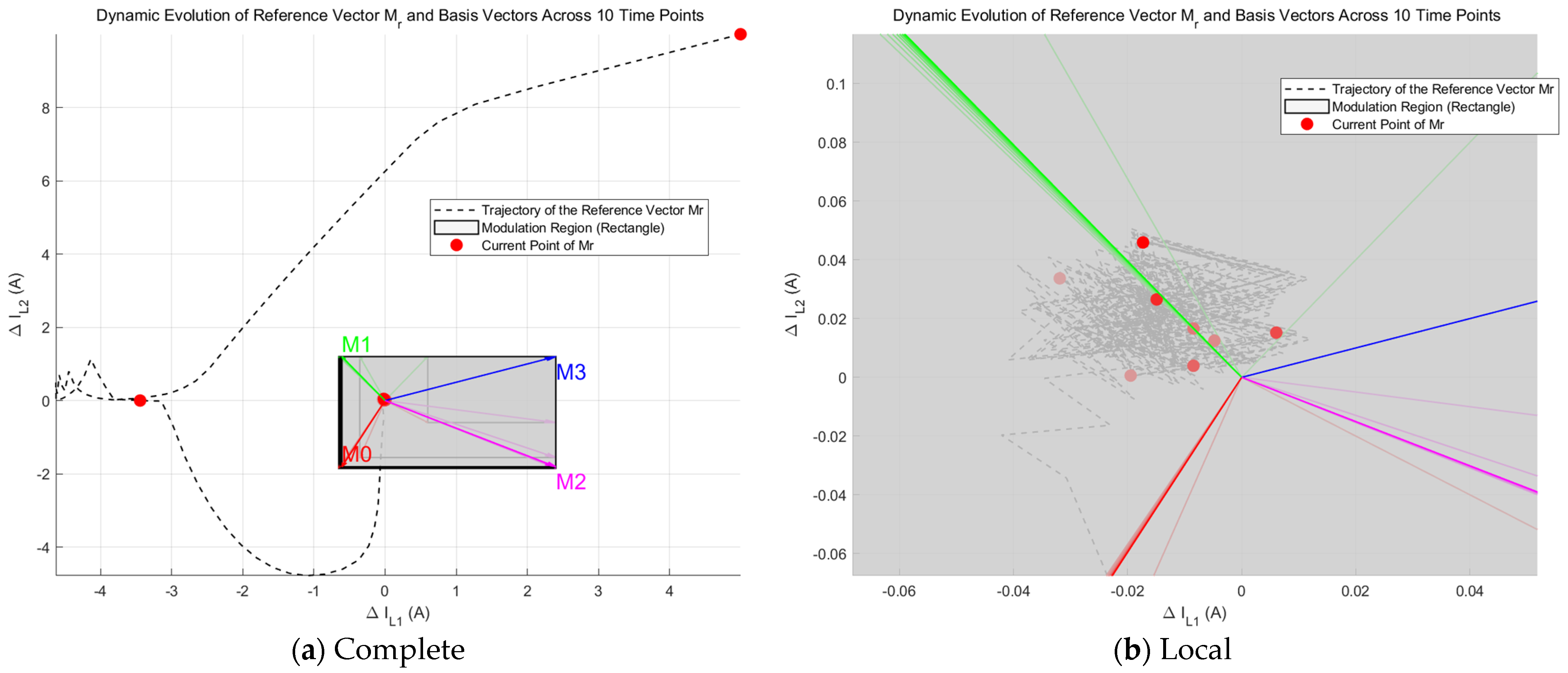
Mode 1 (DISO): The power provided by the photovoltaic port panel is lower than the DC load requirement, and the energy storage battery discharges to the load. The output power of the photovoltaic port is 120 W, corresponding to an output inductor current of 5 A at the photovoltaic port; the load power is 180 W, meaning that the energy storage port output power is 60 W. The simulation time is 10 ms. As shown in Figure 10, 10 time nodes (with an interval of 1 ms between each time point) are selected to plot a vector diagram during the modulation process to verify the effectiveness of the modulation strategy. The gray dashed line represents the complete historical trajectory of the reference vector M_r throughout the simulation. The changing gray translucent rectangles are the modulation regions formed by the four basic vectors M₀, M₁, M₂, and M₃ at the selected 10 time points. It can be observed that each time point has a corresponding symmetric rectangular modulation region. The red solid circles represent the specific positions of the reference vector M_r at each time point. According to the proposed control method of forming the reference vector by proximity and multi-vector synthesis, it can be found that the system basically reaches a stable operating state within 2 ms after startup, with the reference vector M_r converging near the origin.

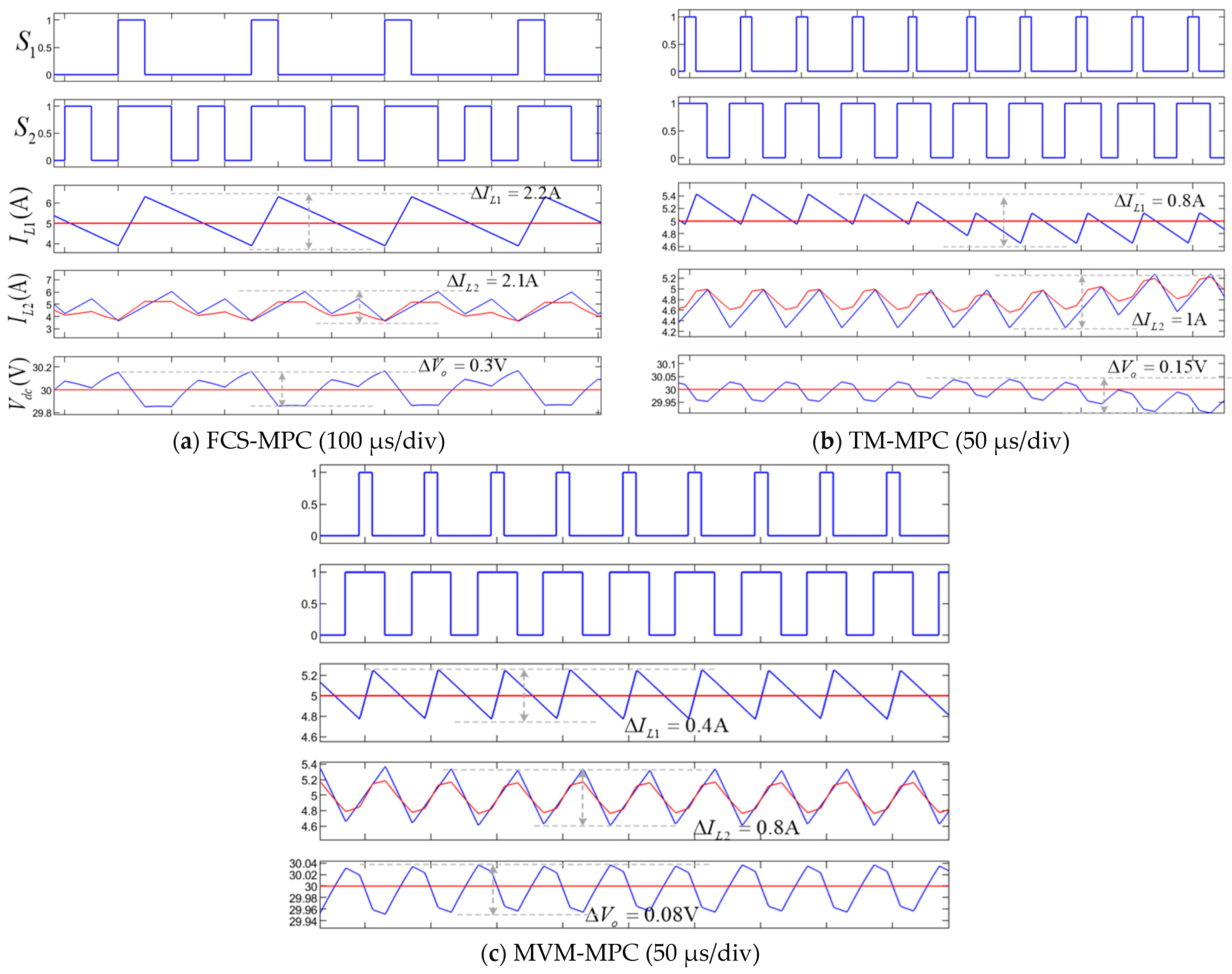
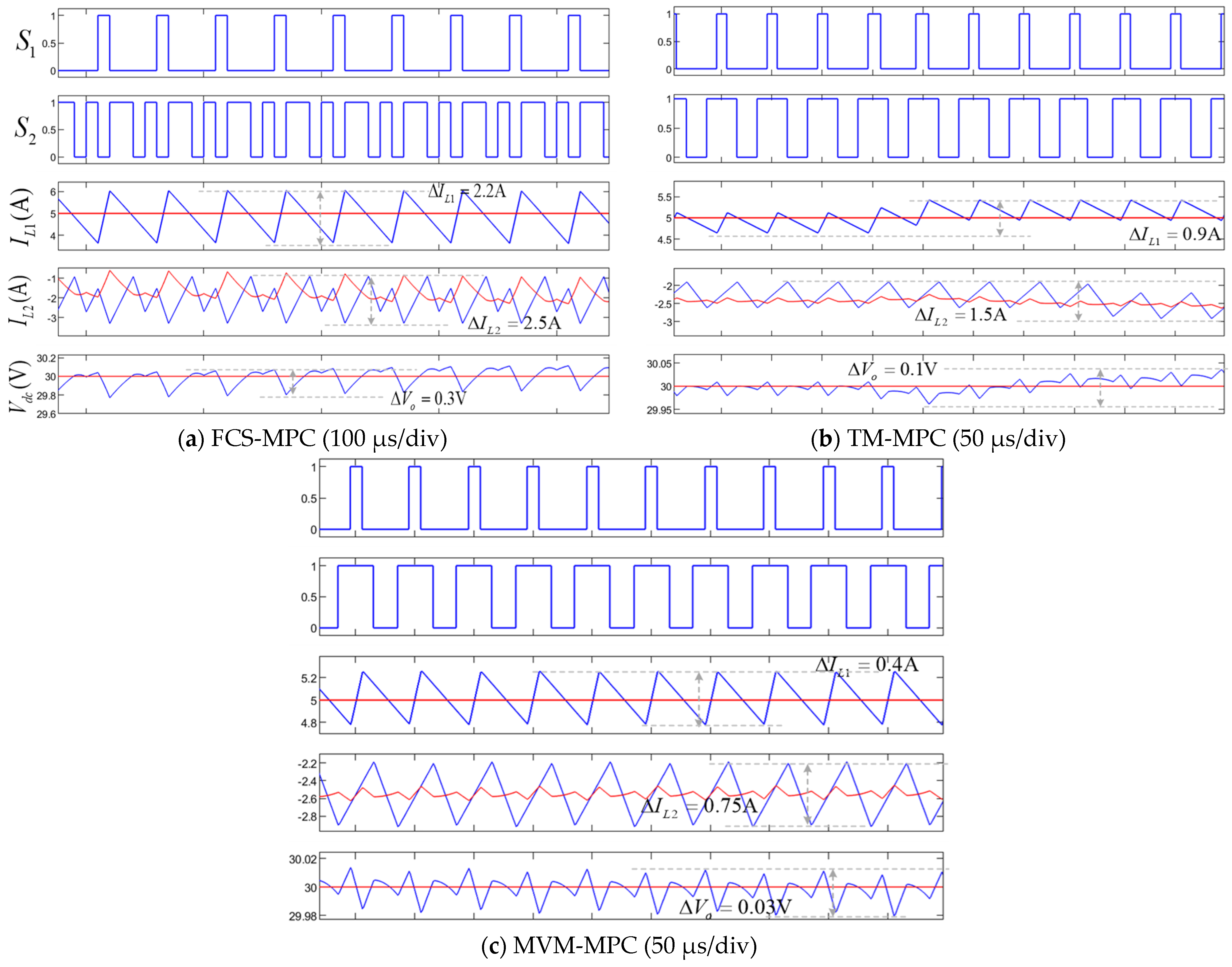
Figure 11 compares the switching actions and control ripple effects of the traditional finite control set MPC (FCS-MPC), traditional modulated MPC (TM-MPC), and the proposed MPC (MVM-MPC). The finite control set MPC method only selects one vector to approximate the reference value, but it cannot achieve zero-error control, and its switching frequency is not fixed, leading to significantly higher current ripple and poor voltage control performance. Although the traditional modulated MPC fixes the switching frequency, it also only selects one vector to approximate the reference value. In contrast, the proposed new modulated MPC can select three vectors (e.g., M₃, M₁, M₀) to achieve error-free control, resulting in significantly reduced current ripples and better voltage control. Meanwhile, the proposed new modulated MPC can achieve a fixed switching frequency, which will simplify filter design.

Table 3. Comparison of voltage and current ripples under different control methods in Mode 1.

Method	$\mathit{\Delta }{\mathit{I}}_{\mathit{L}1}$	$\mathit{\Delta }{\mathit{I}}_{\mathit{L}2}$	$\mathit{\Delta }{\mathit{V}}_{\mathit{d}\mathit{c}}$
FCS-MPC	$2.2 \mathrm{A}$	$2.1 \mathrm{A}$	$0.3 \mathrm{V}$
TM-MPC	$0.8 \mathrm{A}$	$1 \mathrm{A}$	$0.15 \mathrm{V}$
MVM-MPC	$0.4 \mathrm{A}$	$0.8 \mathrm{A}$	$0.08 \mathrm{V}$

summarizes the comparison of voltage and current ripples under different control modes. It can be seen that with the proposed control method, the current ripple and DC bus voltage ripple are both significantly reduced, benefiting from multi-vector analysis and the fixed switching frequency.

Mode 2 (SIDO): The power provided by the photovoltaic port exceeds the DC load power requirement, and the energy storage battery is charged. The output power of the photovoltaic port is 120 W, corresponding to an output inductor current of 5 A at the photovoltaic port; the load power is 90 W, meaning the input power of the energy storage port is 30 W. Similarly, for Mode 2, the simulation time is 0.01 s. As shown in Figure 12, 10 time nodes are selected to plot a vector diagram during the modulation process to verify the effectiveness of the modulation strategy. It can also be observed that the system basically reaches a stable operating state within 2 ms after startup, with the reference vector converging near the origin. Similarly, as shown in Figure 13, comparing different control methods, the proposed new modulated MPC method can achieve significant improvement in control performance under the conditions of fixed switching frequency and multi-vector modulation. Specific ripple comparisons are presented in

Table 4. Comparison of voltage and current ripples under different control methods in Mode 2.

Method	$\mathit{\Delta }{\mathit{I}}_{\mathit{L}1}$	$\mathit{\Delta }{\mathit{I}}_{\mathit{L}2}$	$\mathit{\Delta }{\mathit{V}}_{\mathit{d}\mathit{c}}$
FCS-MPC	$2.2 \mathrm{A}$	$2.5 \mathrm{A}$	$0.3 \mathrm{V}$
TM-MPC	$0.9 \mathrm{A}$	$1.5 \mathrm{A}$	$0.1 \mathrm{V}$
MVM-MPC	$0.4 \mathrm{A}$	$0.75 \mathrm{A}$	$0.03 \mathrm{V}$

.

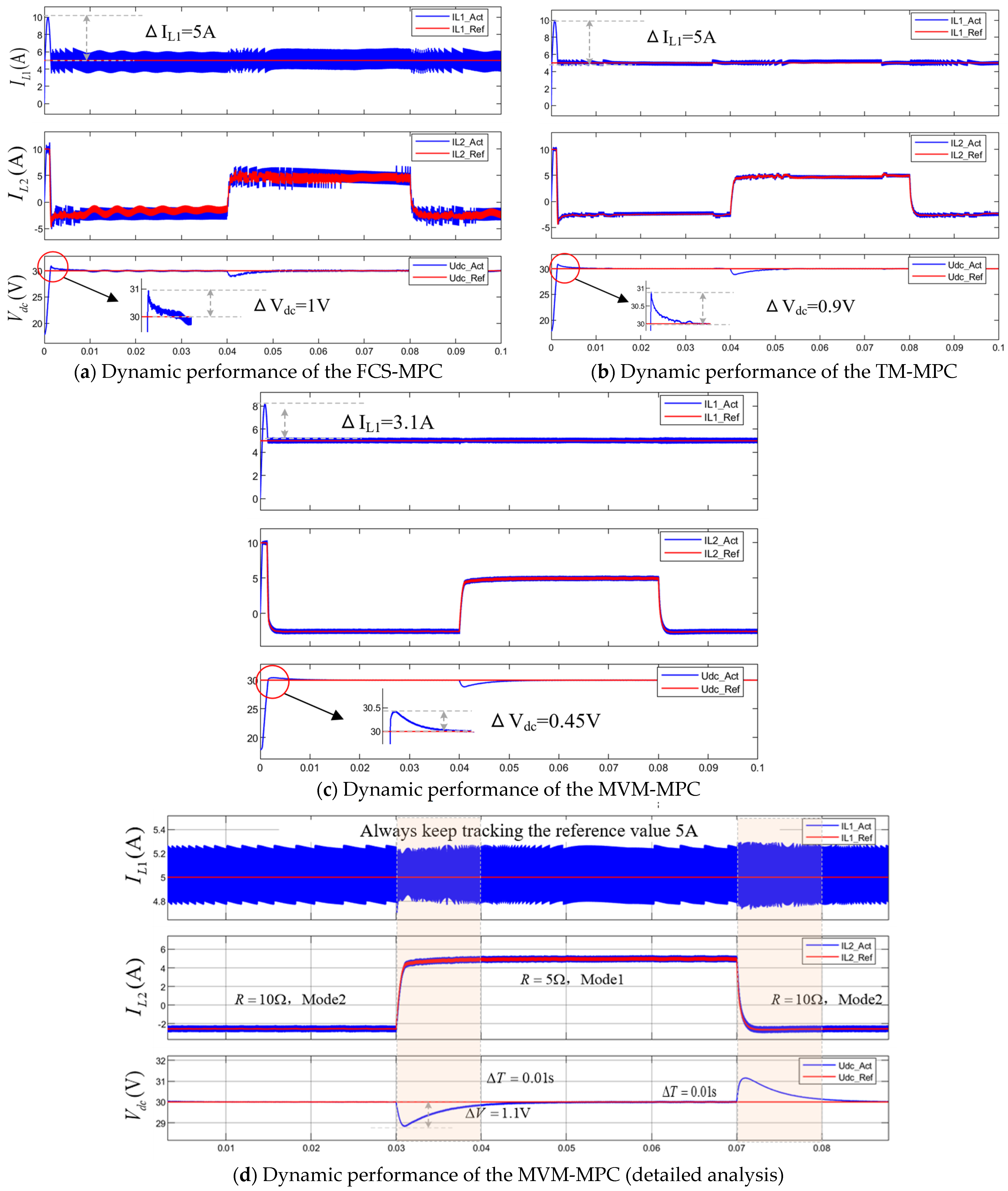
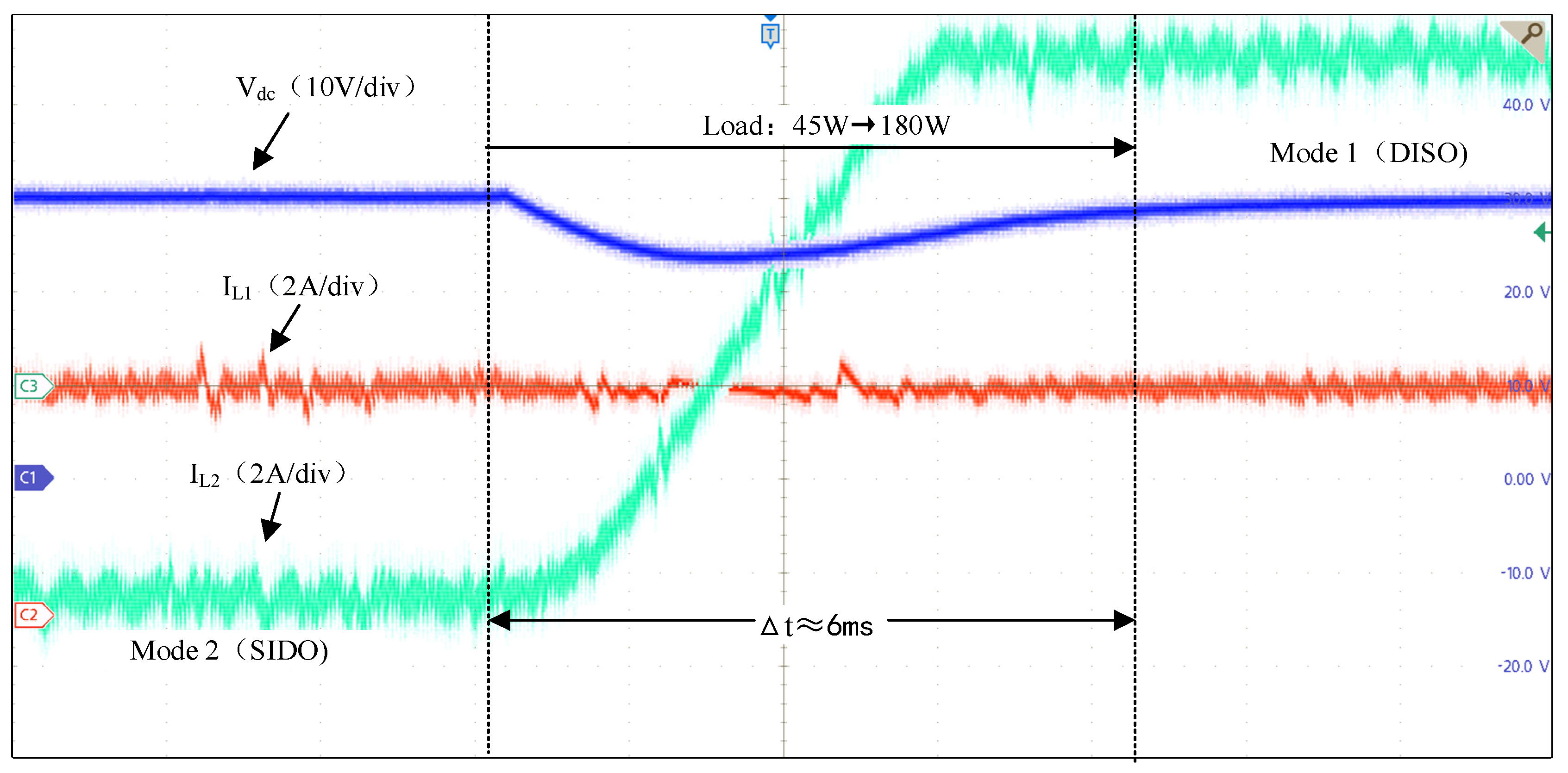
Further, to verify the dynamic performance of the proposed new modulated MPC, a dynamic load simulation was conducted, where the photovoltaic port voltage was 24 V and the reference current value was 5 A, with the load resistance varying between 5 ohm and 10 ohm. The inductor current at the energy storage terminal is limited by the range of −10 A to 10 A. Figure 14 compares the dynamic performance between the conventional FCS-MPC, TM-MPC, and MVM-MPC. Under the condition of consistent parameters of the PI voltage outer loop, a comparison of different control methods reveals that the proposed MPC exhibits significantly smaller voltage overshoots during the startup phase and mode-switching processes. Additionally, the current overshoots on both sides are also reduced. However, there is no significant difference in the regulation time, primarily because the PI controller plays a dominant role in this aspect. As shown in Figure 14d, the photovoltaic port consistently tracks its reference value of 5 A with almost no fluctuations. The battery can quickly and smoothly adjust its charging and discharging states according to the load conditions, with a transient adjustment time of only 0.01 s, without any current overshoot or controller adjustments.

5. Analysis of Experimental Results

5.1. Overview of the Experimental Platform

To verify the effectiveness of the proposed strategy in this paper, a hardware-in-loop (HIL) experimental platform was built, in which the main circuit is simulated by a star-sim simulator, while the control strategy is implemented using a real DSP controller (DSP28335) for verification. This is a common practice to validate the innovation of the control strategy and does not involve issues related to implementation costs [21,22]. The hardware of the three-port DC–DC converter is simulated by the MT 6060-5 real-time simulator, a power electronics hardware-in-the-loop simulation platform. The controller uses a TMS320F28335 DSP from TI (Texas Instruments, Texas Instruments, Dallas, TX, USA). The experimental platform for the three-port DC–DC converter is shown in Figure 15, mainly including the MT 6060-5 real-time simulator, a host computer for the real-time simulator, a TMS320F28335 controller, a host computer for the controller, and an oscilloscope.

5.2. Experimental Results

Mode 1 (DISO): The power provided by the photovoltaic port is lower than the DC load power requirement, and the energy storage port outputs power to the load. The output power of the photovoltaic port is 120 W, with a reference value of 5 A for the output inductor current of the photovoltaic port; the DC load voltage is 30 V, and the load power is 180 W, meaning the energy storage port output power is 60 W. The specific experimental waveforms are shown in Figure 16 and Figure 17. Benefiting from the fixed switching frequency and multi-vector modulation, it can be observed that the inductor current ripple of the photovoltaic port is approximately 0.5 A, the inductor current ripple of the energy storage port is approximately 0.9 A, and the DC bus load voltage ripple is approximately 0.1 V. The symmetry and low amplitude of the ripples verify the rationality of the multi-vector modulated model predictive control method, ensuring that the error vector theoretically approaches zero.

Mode 2 (SIDO): The power provided by the photovoltaic port is higher than the DC load requirement, and the photovoltaic port simultaneously outputs power to both the energy storage port and the load. The output power of the photovoltaic port is 120 W, i.e., the reference value for the photovoltaic port output inductor current is 5 A; the load power is 45 W, meaning the input power of the energy storage battery port is 75 W. The specific waveforms are shown in Figure 18 and Figure 19. Benefiting from the fixed switching frequency and multi-vector modulation, the inductor current ripple of the photovoltaic port is approximately 0.45 A, the inductor current ripple of the energy storage port is approximately 0.8 A, and the DC bus load voltage ripple is approximately 0.05 V.

Furthermore, to verify the dynamic performance of the proposed new modulated MPC, a dynamic load change experiment was conducted, where the photovoltaic port voltage was 24 V, the reference current value was 5 A, and the load suddenly changed from 45 W to 180 W. As shown in Figure 20, the photovoltaic port maintained the tracking of its reference value of 5 A at all times with almost no fluctuations. This indicates that the new modulated MPC had an extremely high control precision and disturbance rejection capability for the photovoltaic port, capable of maintaining the stability of photovoltaic energy output during severe load changes and reflecting the robustness and reliability of the control strategy in handling dynamic tracking of the photovoltaic port.

Meanwhile, the battery can quickly and smoothly adjust its charging and discharging states according to load conditions, with a transient adjustment time of only 6 ms. The rapid adjustment demonstrates that the controller can sense load changes in real time and quickly adjust the power output of the energy storage system, while the smooth transition reflects the control algorithm’s precise regulation of the charging and discharging process of the energy storage device. This avoids damage to the energy storage equipment caused by current surges and verifies the stability and self-adaptability of the control strategy during dynamic processes, as it can adapt to sudden load changes without additional control parameter adjustments.

6. Conclusions

This paper addresses the coordinated control problem of a three-port DC–DC converter with two bidirectional DC–DC converters in parallel. By analyzing and comparing the finite control set MPC (FCS-MPC) and the traditional modulated MPC (TM-MPC), a modulation-based model predictive control method based on vector analysis is proposed. By introducing reference vector synthesis and duty cycle optimization, the problems of fixed switching frequency, large tracking error of FCS-MPC and large tracking error of traditional TM-MPC are solved. The simulation and experimental results show that the fixed switching frequency and multi-vector modulation technology perform excellently in the cooperative control of multi-power ports. The ripple indexes of all physical quantities are better than expected. By synthesizing the reference vector with three basic vectors, the theoretical control error is close to zero. Compared with FCS-MPC, the current ripple is reduced by 61.90–81.82% and the voltage ripple is reduced by 73.33–90% under different working modes. Compared with TM-MPC, the current ripple is reduced by 20–50% and the voltage ripple is reduced by 46.67–70% under different working modes (see Table 3 and Table 4). The rationality of the theoretical design and control strategy is verified, which provides a reliable experimental basis for the engineering application of the photovoltaic energy storage composite system. It shows that the system achieves good performance in power distribution, dynamic response, and stability.

Furthermore, compared to the other two typical MPC methods (which simply traverse all possible options to find the optimal solution), it may require fewer computation steps. However, it places higher demands on computational capabilities and is only suitable for processors with matrix operation capabilities.