Article

Energy-Efficient Prediction of Carbon Deposition in DRM Processes Through Optimized Neural Network Modeling

1
Department of Energy and Power Engineering, Tsinghua University, Beijing 100084, China
2
Zhongyuan Electric Laboratory, Xuchang 461000, China
*
Author to whom correspondence should be addressed.
Energies 2025, 18(12), 3172; https://doi.org/10.3390/en18123172
Submission received: 21 May 2025 / Revised: 10 June 2025 / Accepted: 13 June 2025 / Published: 17 June 2025

Abstract

:
Methane dry reforming (DRM) offers a promising route by converting two greenhouse gases into syngas, but catalyst deactivation through carbon deposition severely reduces energy efficiency. While neural networks offer potential for predicting carbon deposition and reducing experimental burdens, conventional random data partitioning in small-sample regimes compromises model accuracy, stability, and generalizability. To overcome these limitations, we conducted a systematic comparison between backpropagation (BP) and radial basis function (RBF) neural network models. Throughout 10 model trials with random trainset splits, the RBF model demonstrated superior performance and was consequently selected for further optimization. Then, we developed a K-fold cross-validation framework to enhance model selection, resulting in an optimized RBF model (RBF-Imp). The final model achieved outstanding performance on unseen test data (MSE = 0.0018, R² = 0.9882), representing a 64% reduction in MSE and a 4.3% improvement in R² compared to the mean performance across 10 independent validations. These results demonstrated significant improvements in the prediction accuracy, model stability, and generalization capability of the small-sample data model, providing intelligent decision-making support for the removal of carbon deposition.

1. Introduction

With the development of the global economy and the advancement of industrialization, energy consumption worldwide has significantly increased over the past century. This has led to a straight climb in carbon emissions, which has intensified climate warming through the greenhouse effect [1]. Consequently, the development of low-carbon technologies has become a global consensus to achieve the “Net Zero Emission” goals [2,3]. The dry reforming of methane (DRM) offers a promising approach by converting CO2 and CH4, two greenhouse gases, into syngas, which is an important feedstock in the energy and chemical engineering. It can be widely utilized in applications spanning electricity generation, gas processing, and fuel production for fuel cells and H2 vehicles [4]. However, coking side reactions often occur during DRM, resulting in carbon deposition on the catalyst surface, which severely decreasing the yield of DRM and reduce the energy utilization efficiency [5,6]. Consequently, this carbon must be promptly removed to regenerate the catalyst and prevent energy waste, highlighting the importance of monitoring carbon deposition during the reaction process. However, the coking process involves a series of complex reactions simultaneously, with Equations (1) and (2) representing two primary reaction pathways [7]. Additionally, the conversion rates of these reactions are influenced by multiple factors, including the reaction temperature, gas flow rate, reactant ratio, and catalyst properties. As a result, extensive experimental efforts are often required to obtain carbon deposit information, which is another source of energy consumption. Furthermore, as the number of influencing factors increases, experimental requirements scale exponentially, leading to prolonged experimental timelines and increased energy costs, thereby posing significant challenges in monitoring carbon deposition.
C H 4 C + 2 H 2 Δ H = 75   k J / m o l
2 C O C + C O 2 Δ H = 171   k J / m o l
Artificial neural networks (ANNs) process large-scale data via bionic neuron structures, establishing nonlinear relationships between multiple inputs and outputs to achieve accurate data prediction. Compared with time-intensive and energy-consuming experiments, ANNs serve as a cost-effective and efficient research approach that is widely applicable to yield prediction and condition optimization in chemical reactions [8,9]. Ayodele et al. employed an ANN model with CH4 partial pressure, CO2 partial pressure, and reaction temperature as inputs, successfully predicting syngas yields in the DRM over a cobalt-based catalyst [10]. This model showed superior performance, with mean squared errors (MSEs) of 1.56 and 2.40 for H2 and CO yield predictions, respectively, which are significantly lower than the results of traditional response surface methodology (14.90 and 10.76, respectively). Alotaibi et al. used computational fluid dynamics (CFD) simulation data as a training set to develop an ANN model and optimized reaction conditions through a multi-objective genetic algorithm [11]. Similarly, Gendy et al. applied a radial basis function (RBF) neural network to construct a predictive model for methane dry reforming over a Ni-Co-Zr-Al catalyst [12]. The RBFNN model exhibited higher coefficient of determination (R2) values compared to conventional response surface models, further validating the effectiveness of ANNs in chemical reaction prediction.
Although attempts have already been made to use artificial neural networks (ANNs) for yield prediction in dry methane reforming (DMR), such as hydrogen production prediction [13], catalyst optimization [14], etc., their application in coke deposition prediction remains limited. Alsaffar et al. established a nonlinear relationship between reaction conditions and coke deposition using ANNs, enabling prediction at different stoichiometric ratios [15]. In the previous studies, we observed that model performance varied significantly across different randomly divided training sets of the same scale. This sensitivity to data partitioning negatively impacted ANN model training, resulting in inconsistent reliability, compromised accuracy, and elevated overfitting risks. However, the amount of experimental data used for model training must be controlled for cost efficiency in industry, which calls for higher data utilization efficiency. Thus, the trade-off between modeling accuracy and data utilization efficiency represents a key challenge in carbon deposition prediction for DRM. Consequently, for a given dataset size, selecting an appropriate model and implementing effective data processing strategies are essential for maximizing model accuracy, stability, and generalization capability.
To address this issue, we developed both backpropagation (BP) neural networks and radial basis function (RBF) neural networks, with temperature, N2 flow rate, and CH4/CO2 molar ratio, as inputs for accurate carbon deposition prediction. Across ten distinct training datasets, the RBF models demonstrated higher average performance than BP neural networks, which are consequently chosen as more suitable models for further optimization. Here we employed K-fold cross-validation as an efficient data processing method, enabling the rapid identification of RBF-Imp as the optimal model configuration. Accompanied by iterative hyperparameter tuning, this approach maximizes the model’s predictive accuracy, stability, and generalization performance. This data processing and model optimization strategy can be extended to predict carbon deposition with limited datasets in other chemical processes (e.g., dry/wet reforming of alkanes, CO2 hydrogenation), offering the potential for process optimization in both experimental and industrial applications.

2. Model Construction Method

2.1. Data Sources

In a fixed-bed experiment, 100 mg of Co/Al₂O₃ catalyst was loaded into a stainless steel reactor for each trial [15]. The mass of carbon deposition under different temperature, N2 flow rate, and CH4/CO2 molar ratio conditions were obtained from reference [15], with a total of 85 data points. These data are organized in Table 1. Before model training, all data were randomly shuffled. Any 65 datapoints were selected as the training set, and the remaining 20 were taken as the test set.

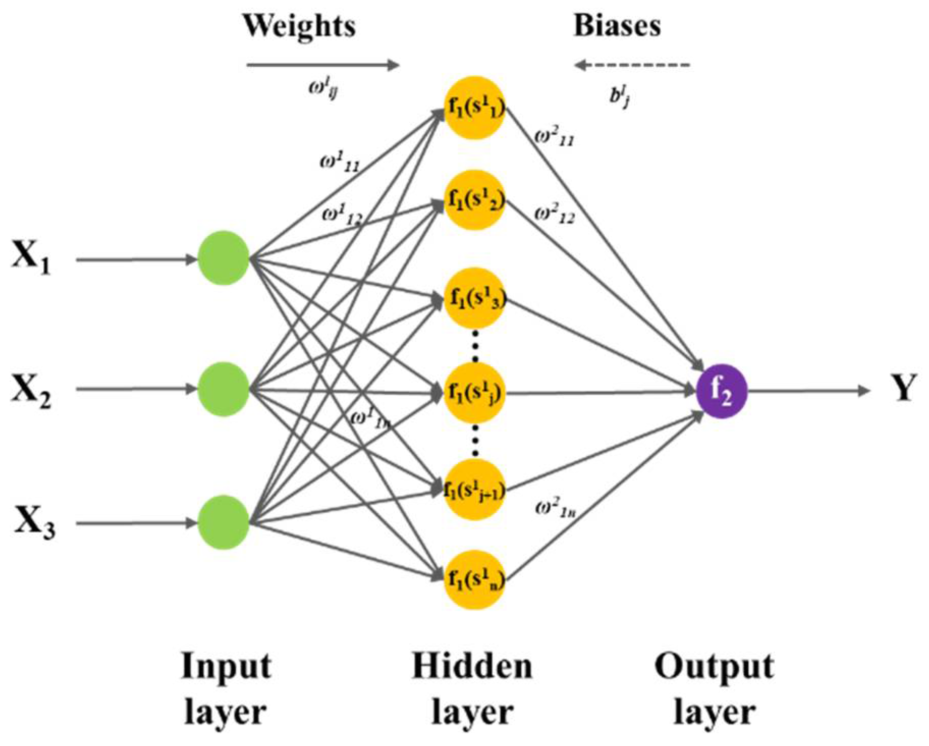
2.2. BP Neural Network Structure and Parameters

The BP neural network is a multilayer feedforward neural network that is trained according to the error backpropagation algorithm. As shown in Figure 1, its structure consists of an input layer, a hidden layer, and an output layer, with each layer composed of multiple neurons interconnected via weights. The computation process of the neurons is represented by Equations (3) and (4), where X i and Y denote the input and output of the neural network, respectively, l represents the layer index, ω l i j denotes the weights of the l-th layer, b l j represents the bias of the l-th layer, and f l ( s l j ) is the activation function of the l-th layer. The specific parameters of this BP model are listed in Table 2. The hidden layer employs the hyperbolic tangent activation function, and the training algorithm adopts the Levenberg–Marquardt algorithm.
s l j = i = 1 n ω l i j X i b l j
y l j = f l ( s l j ) = f l ( i = 1 n ω l i j X i b l j )

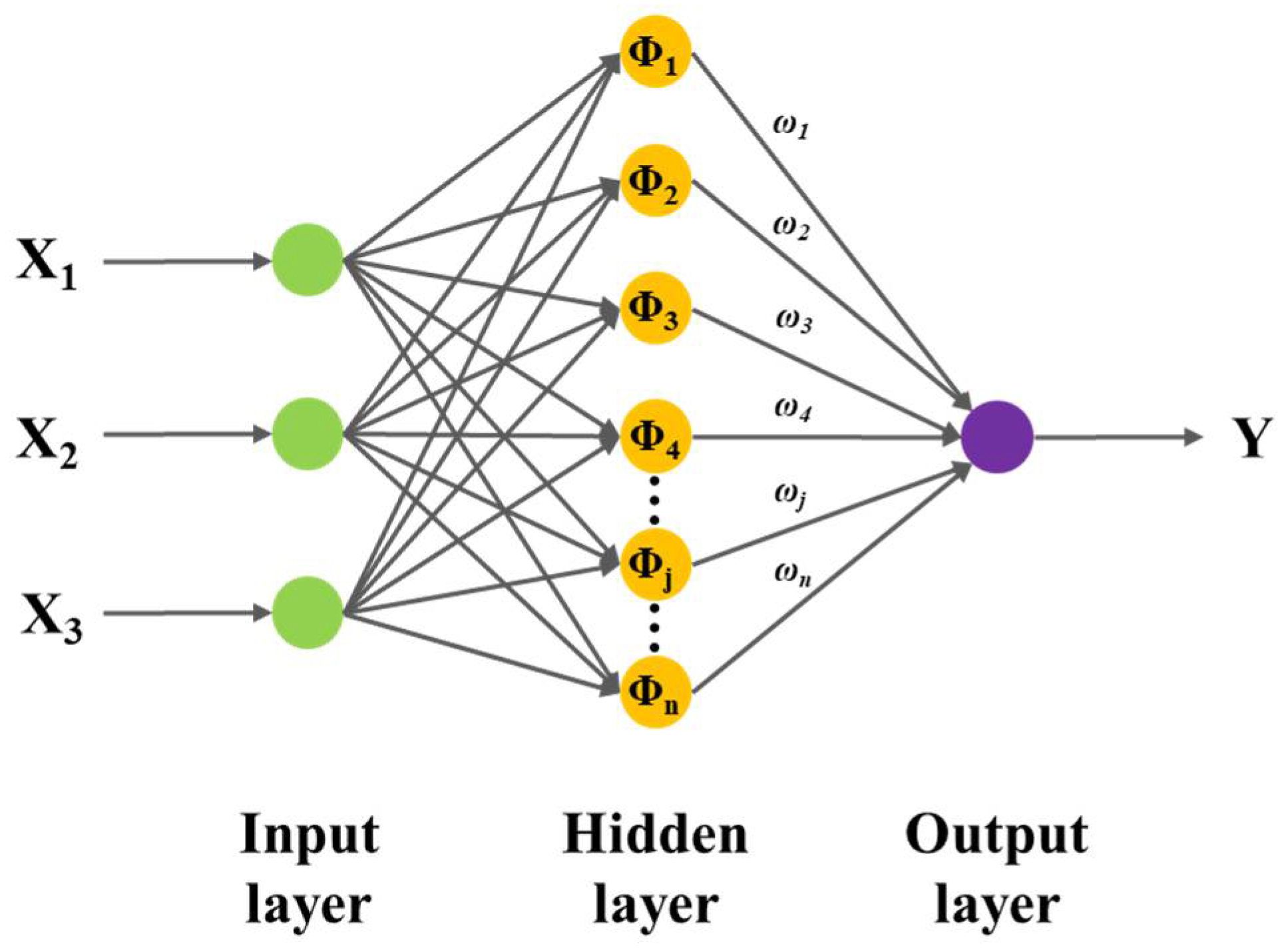
2.3. RBF Neural Network Structure and Parameters

The RBF neural network adopts radial basis functions as its activation functions and is a type of feedforward neural network. Its basic structure is illustrated in Figure 2. Here, the input layer performs a nonlinear mapping from X i to ϕ i ( X ) , while the output layer executes a linear mapping from ϕ i ( X ) to Y . The computational process of its neurons is described by Equations (5) and (6). In the equations, ϕ i ( X ) represents the radial basis function, and σ denotes the spread parameter of the radial basis function. Compared with the BP neural network, the RBF neural network does not require error backpropagation or iterative updates in the output layer, thus accelerating the learning process while avoiding the issue of local minima. The parameters of the model developed in this study are listed in Table 3. During the iterative process, the number of neurons is gradually increased until the target error (0.001) is achieved. The maximum number of neurons is set to 65, matching the length of the training set. The iteration stops as soon as either of these end conditions is met.
Y = g ( X ) = i = 1 n ω i ϕ i ( X )
ϕ i ( X ) = exp ( | | X X i | | 2 σ 2 )

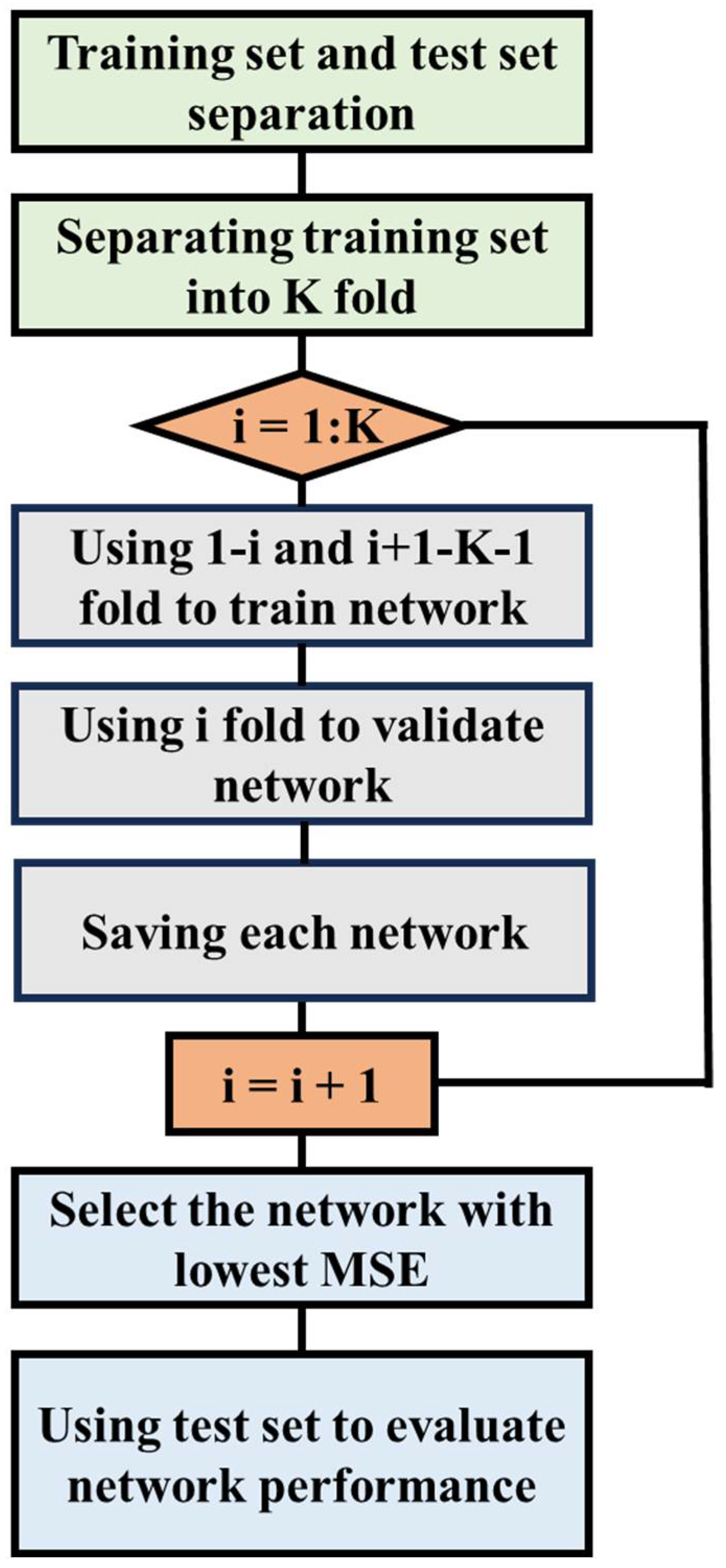
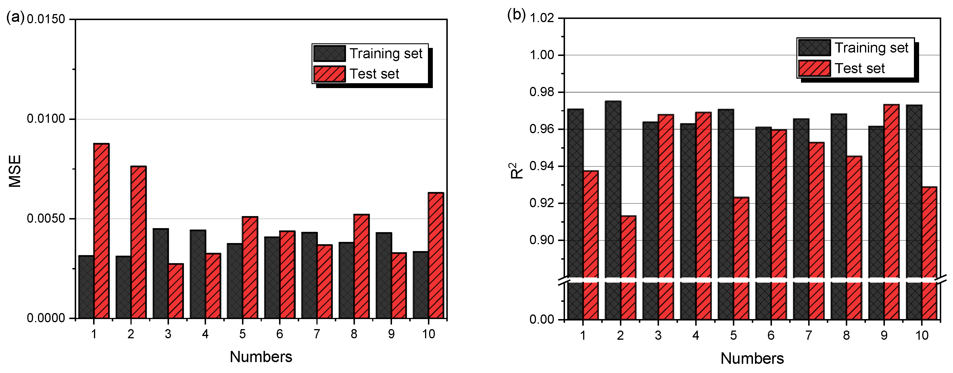
2.4. K-Fold Cross-Validation Optimization Model

To reduce the influence of random training set partitioning, we employed a K-fold cross-validation approach during model training (Figure 3). The dataset was initially split into 65 training samples and 20 test samples, with the training set further divided into K folds. The influence of dataset size on model performance is presented in Table S1, which indicates that the effect is limited when the training set size ranges between 40 and 60. Based on prior research, we set K = 5 as it provides a good balance between selection reliability and computational cost [16,17]. In each cross-validation cycle, K–1 folds were used for network training, while the remaining fold served as the validation set. The model from each cycle was saved, and the one with the lowest mean squared error (MSE) was selected. Finally, this optimal model was evaluated on the test set (unseen external data) to assess its generalization ability.
For each training cycle, a proper spread parameter was selected based on the input data characteristics to maximize prediction performance while minimizing the bias introduced by model configuration. The spread parameter is a critical hyperparameter in RBF neural networks, defining the width of the radial basis function. It governs the function’s response range and directly influences the model’s generalization ability and overall performance. Therefore, appropriate spread parameters were selected to balance model complexity and generalization performance.
By tuning the training data and iteratively adjusting the spread parameter, this K-fold cross-validation method enables robust hyperparameter optimization within an existing dataset and neural network architecture. The final model, RBF-Imp, is chosen to achieve the optimal balance between accuracy and generalization, thereby effectively mitigating the effects of data noise and overfitting.

2.5. Model Performance Evaluation

The performance of the neural network model was evaluated using the mean squared error (MSE) and the coefficient of determination (R²), as defined in Equations (7) and (8), respectively. The MSE measures the average squared deviation between predicted and actual values, reflecting the prediction accuracy of the model. R2 quantifies the proportion of variance in the dependent variable that is predictable from the independent variables, indicating the model stability and prediction precision. These metrics provide complementary insights: while MSE directly assesses prediction errors, R2 evaluates the model’s ability to explain data variability, thereby ensuring a comprehensive performance assessment. Additionally, Figure S1 presents the sensitivity analysis of the RBF model, conducted with 2% deviations over 200 iterations.
M S E = 1 n i = 1 m ( y i y ^ i ) 2
R 2 = 1 i ( y ^ i y i ) 2 i ( y ¯ i y i ) 2

3. Results and Discussion

3.1. Relative Factors of Carbon Deposition Quantity

As shown in Figure 4, the N2 flow rate, CH4/CO2 molar ratio, and temperature all exhibit significant effects on carbon deposition in dry methane reforming. To validate the correlation between the input and output variables in the neural network model, response surface plots were generated by holding one variable constant while varying the other two. This study reveals that at a fixed temperature of 750 °C, lower N2 flow rates and lower CH4/CO2 molar ratios lead to increased carbon deposition. This is because under the low N2 flow rate conditions, the contact time between CH4 and CO2 with the catalyst is prolonged. Additionally, the lower molar ratio of CH4 to CO2 indicates a higher content of CO2, which leads to an increase in the local amount of CO and accelerates the Boudouard reaction, thereby increasing the carbon deposition on the catalyst. When the N2 flow rate remained at 10 mL/min, as the temperature increased, the molar ratio of CH4 to CO2 decreased, and the carbon deposition became more severe. This trend indicates that in high-temperature environments, the increase in CO2 content leads to an intensification of the carbon deposition reaction. Furthermore, when the molar ratio of CH4 to CO2 is fixed at 1.25, a lower N2 flow rate and a higher temperature will promote the carbon deposition. This might be because under high-temperature and low-N2 flow conditions, the cracking reaction of CH4 becomes more intense, thereby resulting in a significant increase in the amount of carbon deposition. Through comprehensive comparison, it can be concluded that the amount of carbon deposition is a function of the N2 flow rate, molar ratio of CH4 to CO2, and temperature, and among these factors, temperature has the most significant impact on the amount of carbon deposition.

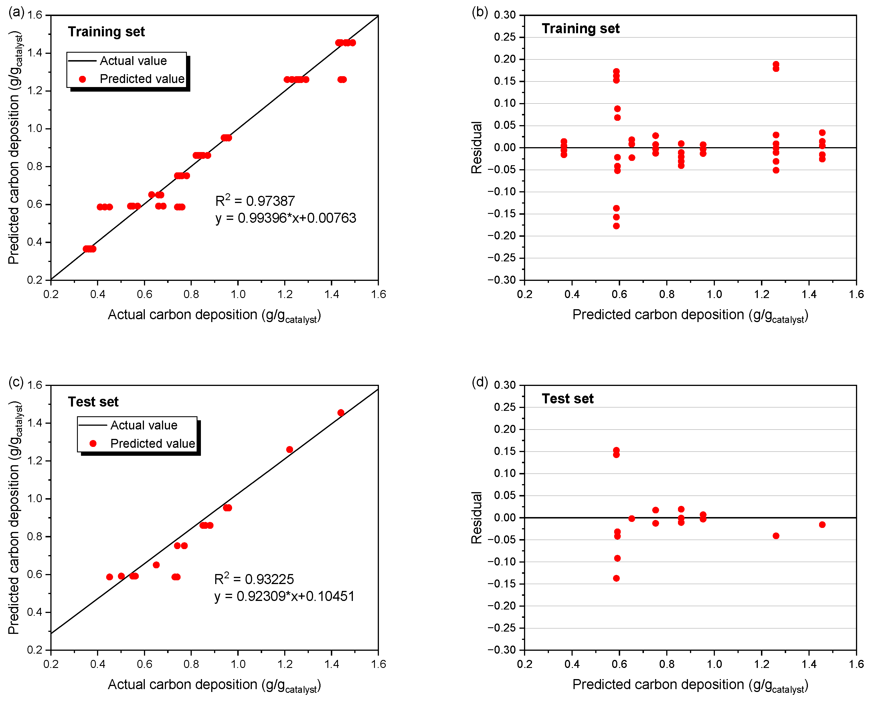
3.2. Predictive Performance of the BP Neural Network

During the model construction process, the training set is used to train the model parameters, while the test set is used to test the prediction performance of the external data. By comparing the prediction results of the training set and the test set, the generalization ability of the model can be evaluated, and the model’s overfitting state status can be determined. In the BP neural network, the number of neurons in the hidden layer determines the width of the neural network. If the number of neurons is too small, it is difficult to achieve accurate prediction, while if the number of neurons is too large, it will increase unnecessary computational load. Therefore, the first step is to optimize the number of neurons in the BP neural network and investigate the impact of this optimization on the prediction accuracy of both the training set and the test set. Figure 5 shows the variation patterns of the mean squared error and the coefficient of determination of the BP neural network training set and test set with respect to the number of neurons in the hidden layer. According to Figure 4a, when n 5 , the MSE of both the training set and the test set is relatively large. When n 5 , the MSE of most of the training set is concentrated around 0.0040, while the MSE of the test set is generally larger than that of the training set, ranging from 0.0040 to 0.0080. As shown in Figure 4b, when n 5 , both the training and testing sets exhibited relatively low R2 values. However, when n 5 , most determination coefficients for the training and testing sets clustered around 0.96, with a minority falling between 0.90 and 0.94. Notably, the testing set contained more data points with lower R2 compared to the training set, which indicates that the model’s predictive performance on unseen data is inferior to that on the training data. Based on the abovementioned analysis, when n = 5 , both the training and test sets exhibit relatively small mean squared errors and high coefficients of determination while maintaining relatively low computational requirements. Therefore, the number of hidden layer neurons was selected as n = 5 .
Figure 6 compares the predicted versus actual values for both the training and test sets in the BP neural network. As shown in Figure 6a, the training set exhibits a strong correlation between predicted and actual values, with the regression line achieving an R2 of 0.97387. Figure 6b demonstrates that the residuals are controlled within 0.20, indicating high prediction accuracy for the training set. For the test set predictions, the R2 value of the regression line decreases to 0.93225 (Figure 6c), suggesting a slightly weaker correlation between predicted and actual values compared to the training set. Nevertheless, the residuals remain within ±0.16 (Figure 6d), confirming that the test set predictions maintain relatively high accuracy.
To investigate the effect of dataset partitioning on model generalization performance on unseen data, we generated 10 distinct random splits, each consisting of 65 training samples and 20 testing samples. Differences in the ten prediction results demonstrate that BP model performance depends heavily on the training data. As shown in Figure 7, the MSE for both the training set and test set remained below 0.0120, while the R2 score stayed above 0.88. Next, we compared the prediction performance between the training and test sets. Figure 7a reveals that 60% of test set’s MSE was higher than that of the training set, indicating poor generalization performance of the BP neural network. Additionally, Figure 7b shows that the variance in R2 for the test set was much larger than that of the training set, suggesting unstable predictions for individual data points. This further demonstrates that the BP neural network’s fitting performance on unseen data lacks stability.

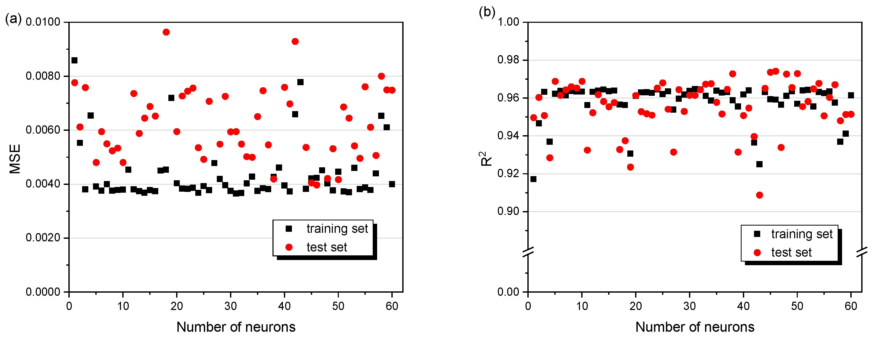
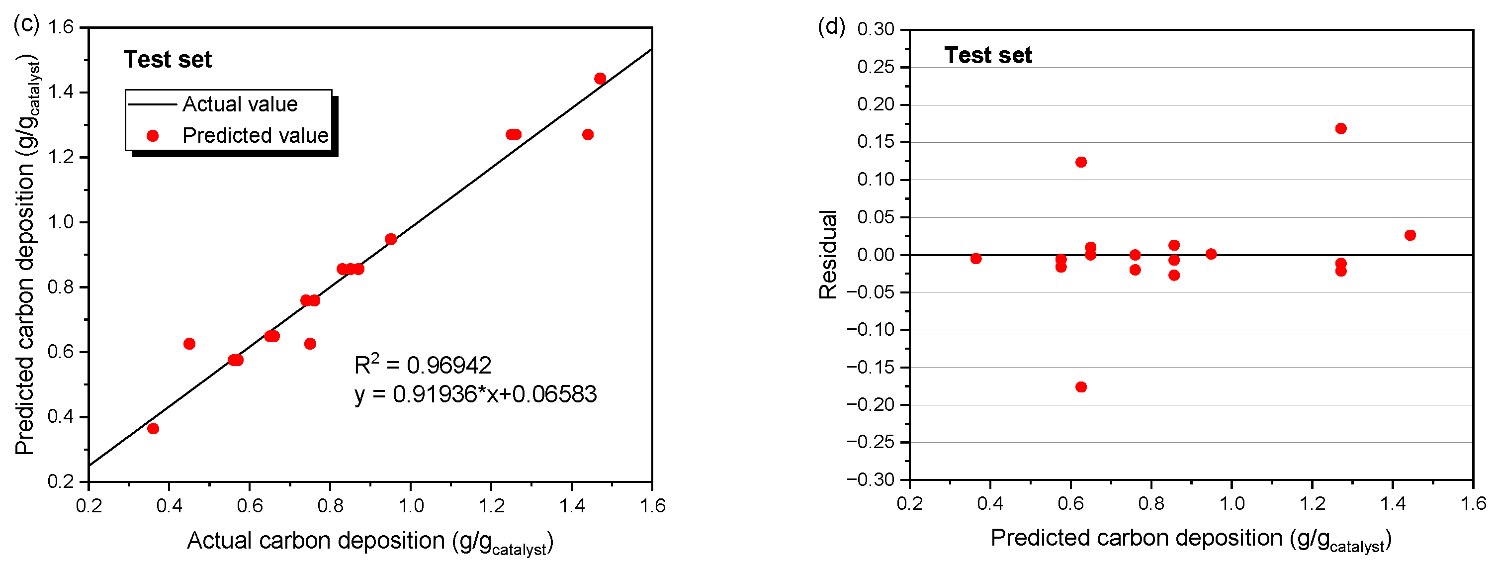
3.3. Predictive Performance of the RBF Neural Network

The RBF neural network was used to verify the data of the training set and the test set in Figure 8. As shown in Figure 8a, the predicted values of the training set of the RBF neural network were compared with the actual values, and it was found that the linearity between the predicted values and the actual values was good, with an R2 of 0.96463 and residuals controlled within ±0.21 (Figure 8b). As shown in Figure 8c, the predicted values and the actual values of the test set of the RBF neural network presented a strong correlation, with an R2 of 0.96942, which was very close to that of the training set. Additionally, the residuals were controlled within ±0.17 (Figure 8d), indicating that this RBF neural network model shows good predictive performance on the test set and the training set simultaneously.
To further verify the generalization ability of the abovementioned results, 10 distinct random splits were trained and tested on the RBF neural network model, as shown in Figure 9. The ten prediction results exhibited noticeable variations, highlighting the impact of the training data composition on the RBF model’s performance. According to Figure 9a, the MSE of the training set and the testing set is within 0.0087, and the errors of the training set and the testing set are close in most cases; however, there are still situations with significant differences. According to Figure 9b, the R2 of the training set is above 0.96, while the R2 of the testing set remains above 0.91. Among these, 70% of the R2 values are between 0.91 and 0.96, indicating that the stability of the prediction of the testing set still has a gap compared to the training set.
Next, the prediction performance of the BP and RBF neural networks trained via 10 random data splittings was compared in Figure 10, and the prediction performance was arranged in ascending order from the lowest to the highest. Figure 10a compares the prediction performance on the unseen test set of both neural networks over 10 runs. The BP network’s maximum MSE reaches 0.0117, whereas the RBF network achieves a lower value of 0.0088. Additionally, for the BP neural network, the MSE range of fluctuation is much larger than that of the RBF network, which means that the prediction stability of RBF network is better. Combined with Table 4, it can be seen that the mean value of the MSE of the BP neural network is larger than that of the RBF neural network. The abovementioned results are consistent and indicate that the RBF neural network has better accuracy and stability in predicting carbon deposition during DRM. In Figure 10b, it can be seen that the minimum R2 of the RBF neural network (0.89) is higher than that of the BP neural network (0.91). Combined with Table 4, it can be seen that the average R2 of the RBF neural network is larger than that of the BP neural network, indicating a higher generalization ability of the RBF neural network. This comparison suggests that the RBF model can be chosen as a better model with higher accuracy, stability, and generalization ability for further optimization.

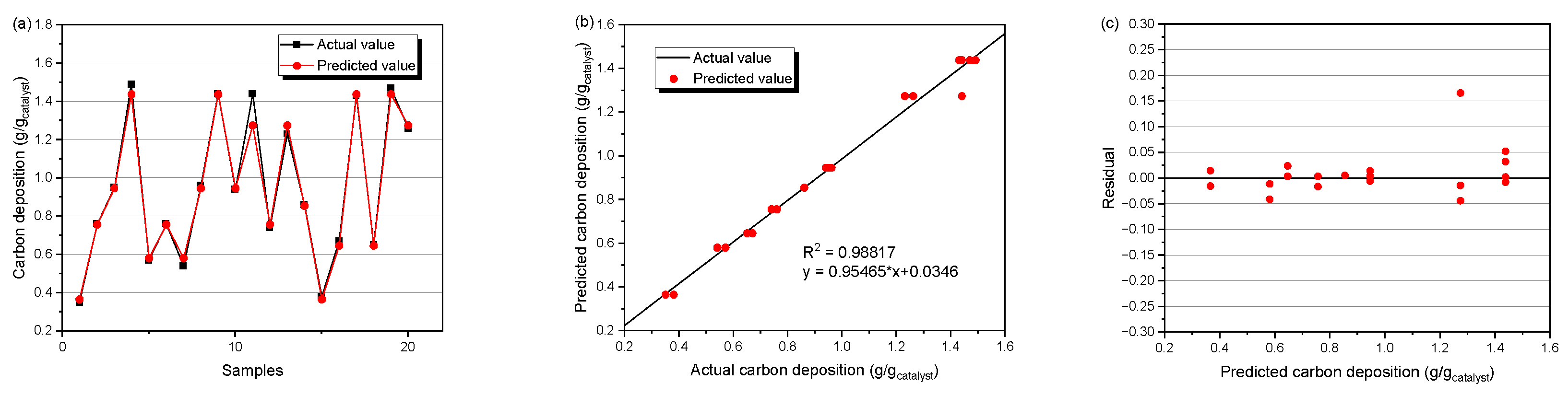
3.4. Prediction Performance of the RBF-IMP Model

To optimize the performance of the RBF model, we employed K-fold cross-validation (Figure 3) to select the best-performing model. The spread parameter was iteratively tuned based on the training set, ultimately yielding the improved RBF model (RBF-Imp). Figure 11 shows the prediction results of the unused test set. Figure 11a compares the experimentally obtained actual values with the model’s predicted values, demonstrating strong agreement between the two. Figure 11b shows that the R2 between the predicted and actual values further improved to 0.9882, which is significantly higher than the results from the 10 random data splits (Figure 10). This indicates the robust prediction stability of the RBF-Imp model across a wide range. Additionally, the residual range narrowed to below 0.16, with most residuals falling below 0.05, confirming high prediction accuracy over the entire carbon deposition range.
A comparative analysis of the BP, RBF, and RBF-Imp models (Table 4) reveals that the optimized RBF-Imp model achieves the lowest mean squared error (MSE = 0.0018) and the highest coefficient of determination (R2 = 0.9882), demonstrating superior accuracy and stability. The results demonstrate the effectiveness of the K-fold cross-validation method in model optimization and selection. This approach maximizes the utility of limited experimental data while identifying the optimal model with strong generalization capability for unseen datasets. This enhanced performance suggests strong potential for extending the model to predict unknown inputs in active processes.

4. Conclusions

In this study, the BP neural network and RBF neural network models were established to predict the carbon deposition on the catalyst surface during the dry reforming of methane. The temperature, N2 flow rate, and CH4/CO2 molar ratio were used as inputs. The results showed that the predicted values obtained by the BP and RBF neural network models were in good consistency and correlation with the experimental values. Through 10 independent validations, the MSE of the BP neural network algorithm was 0.0063, and the R2 was 0.9426, while the MSE of the RBF neural network algorithm was 0.0050, and the R2 was 0.9471. The K-fold cross-validation method was used to optimize and select an improved RBF neural network. The RBF-Imp model has an MSE as low as 0.0018, and the R2 could reach up to 0.9882, indicating that the accuracy and stability of the model were further improved. This model optimization and selection strategy can be generalized to other prediction tasks, thereby enhancing data utilization efficiency and offering a systematic approach for improving model performance under constrained data scale conditions.

Supplementary Materials

The following supporting information can be downloaded at: https://www.mdpi.com/article/10.3390/en18123172/s1, Figure S1: Sensitivity analysis of RBF model (2% deviation, 200 iterations), Table S1: Comparative results of influence of dataset size on RBF model performance.

Author Contributions

Conceptualization, R.F.; methodology, R.F. and T.Z.; software, Z.X.; formal analysis, R.F. and Z.X.; investigation, R.F. and X.H.; resources, R.F. and X.H.; data curation, R.F.; writing—original draft preparation, R.F.; writing—review and editing, T.Z.; supervision, T.Z., M.Z. and H.Y.; funding acquisition, H.Y. All authors have read and agreed to the published version of the manuscript.

Funding

This work was financially supported by the National Natural Science Foundation of China (No. 52306029) and the Zhongyuan Electric Laboratory (No.zn20250401).

Data Availability Statement

Data is contained within the article.

Conflicts of Interest

The authors declare no conflicts of interest.

Abbreviations

The following abbreviations are used in this manuscript:
ANNArtificial neural network
BPBackpropagation
CFDComputational fluid dynamics
DRMDry reforming of methane
MSEMean squared error
RBFRadial basis function
R2Coefficient of determination

References

  1. Liu, Z.; Deng, Z.; Davis, S.J.; Ciais, P. Global carbon emissions in 2023. Nat. Rev. Earth Environ. 2024, 5, 253–254. [Google Scholar] [CrossRef]
  2. Mohammed, S.; Eljack, F.; Al-Sobhi, S.; Kazi, M.-K. A systematic review: The role of emerging carbon capture and conversion technologies for energy transition to clean hydrogen. J. Clean. Prod. 2024, 447, 141506. [Google Scholar] [CrossRef]
  3. Wang, Z.; Mei, Z.; Wang, L.; Wu, Q.; Xia, C.; Li, S.; Wang, T.; Liu, C. Insight into the activity of Ni-based thermal catalysts for dry reforming of methane. J. Mater. Chem. A 2024, 12, 24802–24838. [Google Scholar] [CrossRef]
  4. Nguyen, D.L.T.; Vy Tran, A.; Vo, D.-V.N.; Tran Nguyen, H.; Rajamohan, N.; Trinh, T.H.; Nguyen, T.L.; Le, Q.V.; Nguyen, T.M. Methane dry reforming: A catalyst challenge awaits. J. Ind. Eng. Chem. 2024, 140, 169–189. [Google Scholar] [CrossRef]
  5. Arora, S.; Prasad, R. An overview on dry reforming of methane: Strategies to reduce carbonaceous deactivation of catalysts. RSC Adv. 2016, 6, 108668–108688. [Google Scholar] [CrossRef]
  6. Vogt, E.T.C.; Fu, D.; Weckhuysen, B.M. Carbon Deposit Analysis in Catalyst Deactivation, Regeneration, and Rejuvenation. Angew. Chem. Int. Ed. 2023, 62, e202300319. [Google Scholar] [CrossRef] [PubMed]
  7. Abdullah, B.; Abd Ghani, N.A.; Vo, D.-V.N. Recent advances in dry reforming of methane over Ni-based catalysts. J. Clean. Prod. 2017, 162, 170–185. [Google Scholar] [CrossRef]
  8. Toyao, T.; Maeno, Z.; Takakusagi, S.; Kamachi, T.; Takigawa, I.; Shimizu, K.-I. Machine Learning for Catalysis Informatics: Recent Applications and Prospects. ACS Catal. 2019, 10, 2260–2297. [Google Scholar] [CrossRef]
  9. Aklilu, E.G.; Bounahmidi, T. Machine learning applications in catalytic hydrogenation of carbon dioxide to methanol: A comprehensive review. Int. J. Hydrogen Energy 2024, 61, 578–602. [Google Scholar] [CrossRef]
  10. Ayodele, B.V.; Khan, M.R.; Nooruddin, S.S.; Cheng, C.K. Modelling and optimization of syngas production by methane dry reforming over samarium oxide supported cobalt catalyst: Response surface methodology and artificial neural networks approach. Clean Technol. Environ. Policy 2016, 19, 1181–1193. [Google Scholar] [CrossRef]
  11. Alotaibi, F.N.; Berrouk, A.S.; Saeed, M. Optimization of Yield and Conversion Rates in Methane Dry Reforming Using Artificial Neural Networks and the Multiobjective Genetic Algorithm. Ind. Eng. Chem. Res. 2023, 62, 17084–17099. [Google Scholar] [CrossRef]
  12. Gendy, T.S.; El-Salamony, R.A.; Alrashed, M.M.; Bentalib, A.; Osman, A.I.; Kumar, R.; Fakeeha, A.H.; Al-Fatesh, A.S. Enhanced predictive optimization of methane dry reforming via ResponseSurface methodology and artificial neural network approaches: Insights using a novel nickel-strontium-zirconium-aluminum catalyst. Mol. Catal. 2024, 562, 114216. [Google Scholar] [CrossRef]
  13. Rahman, M.H.; Biswas, M. Modeling of Dry Reforming of Methane Using Artificial Neural Networks. Hydrogen 2024, 5, 800–818. [Google Scholar] [CrossRef]
  14. Ameen, S.; Farooq, M.U.; Samia; Umer, S.; Abrar, A.; Hussnain, S.; Saeed, F.; Memon, M.A.; Ajmal, M.; Umer, M.A.; et al. Catalyst breakthroughs in methane dry reforming: Employing machine learning for future advancements. Int. J. Hydrogen Energy 2025, 141, 406–443. [Google Scholar] [CrossRef]
  15. Alsaffar, M.A.; Ayodele, B.V.; Mustapa, S.I. Scavenging carbon deposition on alumina supported cobalt catalyst during renewable hydrogen-rich syngas production by methane dry reforming using artificial intelligence modeling technique. J. Clean. Prod. 2020, 247, 119168. [Google Scholar] [CrossRef]
  16. Marcot, B.G.; Hanea, A.M. What is an optimal value of k in k-fold cross-validation in discrete Bayesian network analysis? Comput. Stat. 2020, 36, 2009–2031. [Google Scholar] [CrossRef]
  17. Fushiki, T. Estimation of prediction error by using K-fold cross-validation. Stat. Comput. 2009, 21, 137–146. [Google Scholar] [CrossRef]
Figure 1. Structure of the BP neural network (Green: input layer neuron; yellow: hidden layer neuron; purple: output layer neuron. Arrows: directions of data flow).
Energies 18 03172 g001
Figure 2. Structure of the RBF neural network (Green: input layer neuron; yellow: hidden layer neuron; purple: output layer neuron. Arrows: directions of data flow.).
Energies 18 03172 g002
Figure 3. Illustration of the K-fold method for model selection.
Energies 18 03172 g003
Figure 4. Influence of N2 flow rate, CH4/CO2 ratio, and temperature on carbon deposition during DRM: (a) Combined influence of N2 flow rate and CH4/CO2 ratio at 750 °C; (b) Combined influence of temperature and CH4/CO2 ratio when N2 flow rate is 10 mL/min; (c) Combined influence of temperature and N2 flow rate when CH4/CO2 ratio is 1.25.
Energies 18 03172 g004
Figure 5. Influence of the number of neurons in the hidden layer on (a) the mean squared error and (b) the coefficient of determination.
Energies 18 03172 g005
Figure 6. (a) Comparison of predicted values and actual values as well as (b) corresponding residuals of the training set, and (c) comparison of predicted values and actual values as well as (d) corresponding residuals of the testing set in the BP neural network.
Energies 18 03172 g006
Figure 7. (a) Mean squared error and (b) coefficient of determination of the training set and test set after 10 independent validations of the BP neural network.
Energies 18 03172 g007
Figure 8. (a) Comparison of predicted values and actual values as well as (b) corresponding residuals of the training set, and (c) comparison of predicted values and actual values as well as (d) corresponding residuals of the testing set in the RBF neural network.
Energies 18 03172 g008aEnergies 18 03172 g008b
Figure 9. (a) Mean squared error and (b) coefficient of determination of the training set and test set after 10 independent validations of the RBF neural network.
Energies 18 03172 g009
Figure 10. (a) Mean squared error and (b) coefficient of determination of the test set after 10 independent validations of the BP and RBF neural network.
Energies 18 03172 g010
Figure 11. Comparison of the test set’s (a) predicted values and actual values, as well as the (b) coefficients of determination and (c) residual values of the predicted values for the RBF-Imp neural network.
Energies 18 03172 g011
Table 1. Experimental data on carbon deposition in dry reforming of methane [13].
NumberCH4/CO2 Molar RatioN2 Flow Rate (mL/min)Temperature (°C)Carbon Deposition (g/gcatalyst)
11.25107501.47
25107500.94
31.25106500.76
45106500.43
51.25107501.43
63.13257000.67
75106500.75
81.25107501.43
95407500.83
101.25406500.68
115106500.45
121.25407501.21
135107500.95
145106500.41
151.25107501.49
161.25407501.23
171.25406500.5
183.13257000.65
195107500.94
205106500.45
215407500.82
221.25107501.44
231.25407501.22
245107500.96
255407500.84
261.25106500.78
271.25406500.57
285407500.85
291.25107501.44
305106500.74
311.25407501.23
321.25107501.46
331.25107501.43
341.25406500.66
351.25406500.55
365406500.35
371.25107501.43
385407500.87
395107500.94
403.125257000.63
411.25106500.77
425106500.73
435406500.36
445407500.88
451.25106500.76
461.25406500.54
473.13257000.65
485107500.94
491.25106500.74
501.25106500.76
511.25407501.25
525406500.37
531.25407501.26
541.25406500.56
551.25406500.57
565406500.35
575407500.87
581.25106500.74
591.25407501.27
605407500.88
615106500.74
625406500.36
635407500.85
645406500.37
655106500.75
661.25406500.55
675406500.36
681.25106500.75
695106500.76
701.25407501.29
715107500.95
725406500.37
735107500.96
745407500.86
751.25107501.47
761.25406500.56
775107500.95
781.25407501.44
791.25407501.45
805107500.96
815406500.38
821.25106500.74
833.13257000.66
841.25106500.76
855406500.37
Table 2. Main parameters of the BP neural network.
Input layerInput parametersTemperature, N2 flow rate, CH4/CO2 ratio
Node number3
Hidden layerLayer1
Node number5
Activation functionHyperbolic tangent function
Training algorithmLevenberg–Marquardt
Output layerOutput parametersCarbon deposition
Node number1
Activation functionLinear transfer function
Error functionMean squared error (MSE)
Table 3. Main parameters of the RBF neural network.
Input layerInput parametersTemperature, N2 flow rate, CH4/CO2 ratio
Node number3
Hidden layerLayer1
Maximum node number65
Target error0.001
Activation functionGaussian basis function
Output layerOutput parametersCarbon deposition
Node number1
Activation functionLinear transfer function
Error functionMean squared error (MSE)
Table 4. Comparison of the predictive performance of the BP, RBF, and RBF-Imp neural networks.
BPRBFRBF-Imp
MSE0.00630.00500.0018
R20.94260.94710.9882
The performance values of the BP and RBF neural networks are based on the means of 10 independent validations.
Disclaimer/Publisher’s Note: The statements, opinions and data contained in all publications are solely those of the individual author(s) and contributor(s) and not of MDPI and/or the editor(s). MDPI and/or the editor(s) disclaim responsibility for any injury to people or property resulting from any ideas, methods, instructions or products referred to in the content.

