Low-Power Constant Current Driver for Stepper Motors in Aerospace Applications

Abstract

Stepper motors are used in satellites for various drive operations that are achieved by custom designs. This paper presents a stepper motor driver for satellite systems. It takes rotor position and phase current as inputs and employs a current subdivision method with back-propagation neural network (BPNN) to achieve constant current control of the motor. The driver can ensure the smooth operation and the positioning accuracy of the motor with a filter wheel that is 0.1944 $\mathrm{kg}·{\mathrm{m}}^2$ in the moment of inertia and satisfy self-adaption of the load without system parameter identification. Compared to the previous scheme, the proposed scheme can reduce the power consumption by about $21.15\%$ when the motor runs at 2 $\mathrm{r}/\mathrm{s}$, which is beneficial to the reduction in the size and the mass of some power supply modules. The performances of the developed driver are implemented on a field programmable gate array (FPGA) circuit board. The experimental results are conducted to verify the claims presented. The proposed scheme can be extended to other stepper motor systems with large moment of inertia loads within spacecraft.

1. Introduction

Stepper motors (SMs) are widely used in aerospace motion mechanisms because of their brushless feature, excellent response to start-up, stopping and reverse, high running precision, reliable structure, and simple control [1,2,3]. Seeing that bipolar motors can produce more torque than unipolar motors with the same size, they are quite suitable for space motion mechanisms, with smaller space size, being more lightweight, and having more required torque. However, their disadvantage is that the control circuit is more complex compared to unipolar motors [4]. Hence, the research of advanced control technology to improve SM drive performance plays an important role in space applications. In view of the reliability of space motion systems and the requirement of easy integration with other systems, one of the main difficulties of SMs is the lack of the drive scheme that matches the mission.

The drive schemes of SMs have been discussed in previous work. Aranjo et al. [5] presented a versatile drive control system of SMs. Kim et al. [6] studied a new position control method of SMs by the microstepping technique. Nevertheless, the drive performance of these schemes is not well tested in practice. Le et al. [7] introduced an effective closed-loop control method for SM drives. However, its implementation requires parameter identification. In addition, the proposed algorithm is executed on an industrial test bench from an outside manufacturer. To improve the current tracking performance of the current subdivision, several feedback control approaches were discussed in [8,9,10,11,12,13]. The position feedback was implemented using encoders to improve current subdivision [14]. However, these approaches require complex calculations. Several schemes using the current subdivision or the combining of the current subdivision with a closed loop were discussed in [15,16,17]. These methods have improved the drive performance of SMs. Nevertheless, they are effective at either low speeds [15] or medium and high speeds [17], but not over all speeds. In view of self-adaption and learning ability, the neural networks (NNs) play a strong role in power electronics and motor drive control [18]. In [19], a recurrent NN-based algorithm is introduced to compute the robust adaptive model predictive speed control law by solving an optimization problem in real-time. In [20], two vector source inverters based on an artificial NN are presented as a new intelligent direct torque control applied to a doubly fed induction motor. Liu et al. [21] proposed a gradient descent algorithm-based B-spline wavelet NN learning adaptive controller for linear motor systems under system uncertainties and actuator saturation constraints. Li [22] proposed a robust control method with NNs to improve three-dimensional tracking performance of the spherical SM system. Tran et al. [23] introduced an adaptive feed-forward proportional-resonant current control strategy with the NN to improve the motion accuracy of the SM. These application cases show that NN algorithms are a powerful tool in motor drive control systems with uncertainties.

In consideration of the ability in processing speed and logical capacity, and the advantages of high performance and high density, FPGA has a significant impact on industrial control systems. The design methodology of control systems based on FPGA is summarized in [24]. Idkhajine et al. [25] introduced an integrated control scheme of synchronous motors based on Actel Fusion FPGA. Muresan et al. [26] designed a fractional order PI controller executed on the FPGA for the direct current (DC) motor speed control. It can be inferred that hardware controllers realized by FPGA with digital structure and easy verification are widely designed in industry.

As seen from previous research, most of the schemes discussed are applicable to lightweight load drives in a good environment. However, the proposed system is located in a harsh aerospace environment containing the wide temperature variation range and complex radiation from gamma rays, high-energy protons, and cosmic rays, which can lead to the failure of low-quality electronic components and single event upset (SEU) of the digital signal processor (DSP) [27], the programmable logic controller (PLC) [28], or the microcontroller unit (MCU) [29], which may result in measurement data loss and function interruption of the drive system. Therefore, in some heavy load drive aerospace systems, these previous schemes can not meet the requirements. It is absolutely necessary for us to propose a new control method and design a drive circuit with high-quality and anti-irradiation electronic components for the SM heavy load drive over the full speed range. As shown in Figure 1, the SM in this paper is used to drive the heavy filter wheel embedded with four optical filters that are used for making the centers of four optical filters be collinear with the center of the light through the hole to enable the infrared detector to measure infrared radiation of the corresponding spectrum from the measured object. In summary, in view of the reliability of the aerospace motion control system, the requirement of easy integration with other electronic systems, and the complex radiation of the aerospace environment, this paper focuses on the design of an FPGA-based SM driver in aerospace applications. The main contributions of this paper are summarized as follows.

$\left(1\right)$

A current subdivision method incorporating BPNN is proposed to ensure stable current regulation of the SM.

$\left(2\right)$

The general measurement methods are presented to accurately detect the rotor position and phase current.

$\left(3\right)$

An FPGA-based SM drive circuit is designed to be suitable for the aerospace environment.

The rest of this paper is organized as follows. Section 2 explains the current stabilization technique employed for the motor. Section 3 describes the hardware implementation on a single FPGA. Section 4 presents the experimental results to confirm the effectiveness of the designed driver. Finally, the conclusion is summarized in Section 5.

2. SM Constant Current Control

Figure 2 shows the structure of the SM system. In Figure 2, $T_{em}$ is the electromagnetic torque $(\mathrm{N}·\mathrm{m})$, $\omega$ is the angular velocity $(\mathrm{rad}/\mathrm{s})$, $T_0$ is the no-load torque $(\mathrm{N}·\mathrm{m})$, $T_w$ is the external disturbance torque $(\mathrm{N}·\mathrm{m})$, $T_l$ is the load torque $(\mathrm{N}·\mathrm{m})$, and $T_h$ is the Hall sensor torque $(\mathrm{N}·\mathrm{m})$.

The dynamic model of the system is expressed as

$$T_{em}-T_0-T_h-T_w-T_l=J{\displaystyle \frac{d\omega }{dt}}+A_v\omega$$

(1)

where J is the moment of inertia $(\mathrm{kg}·{\mathrm{m}}^2)$, and $A_v$ is the viscous friction coefficient $(\mathrm{N}·\mathrm{m}·\mathrm{s}/\phantom{\mathrm{s}\mathrm{rad}}\mathrm{rad})$.

The angular velocity of the motor can be calculated as

$$\omega ={\displaystyle \frac{d\theta }{dt}}$$

(2)

where $\theta$ is the rotor position angle $\left(\mathrm{rad}\right)$.

The sum of $T_0$, $T_h$, $T_w$, and $T_l$ is denoted as $T_n$ that is a nonlinear function, which is written as

$$T_n=T_0+T_h+T_w+T_l$$

(3)

Based on Equations (1)–(3), the system dynamic model is rewritten as

$$T_{em}-T_n=J{\displaystyle \frac{d^2\theta }{d{t}^2}}+A_v{\displaystyle \frac{d\theta }{dt}}$$

(4)

If the reference position signal ${\theta }_r$ is given, then the position signal error is defined by $e_r={\theta }_r-\theta$, and the tracking error is expressed as [30]

$$r={\displaystyle \frac{d{e}_r}{dt}}+\mathrm{\Lambda }{e}_r$$

(5)

where $\mathrm{\Lambda }$ is a design parameter that is a positive constant. This parameter plays a decisive role in controlling the position and speed of the motor.

By using $e_r$, Equations (4) and (5), the system dynamic model is transformed to be

$$J{\displaystyle \frac{dr}{dt}}=-A_{v}r-T_{em}+F\left(\mathbf{x}\right)$$

(6)

where $F\left(\mathbf{x}\right)$ is a nonlinear function with respect to J, $A_v$, $T_n$, ${\theta }_r$, and $e_r$

$$F\left(\mathbf{x}\right)=J\left({\displaystyle \frac{d^2{\theta }_r}{d{t}^2}}+\mathrm{\Lambda }{\displaystyle \frac{d{e}_r}{dt}}\right)+A_v\left({\displaystyle \frac{d{\theta }_r}{dt}}+\mathrm{\Lambda }{e}_r\right)+T_n$$

(7)

where the term $\mathbf{x}$ contains all the signals with respect to time and can be defined as

$$\mathbf{x}\equiv {\left[\begin{array}{ccccc}{\theta }_r& {\displaystyle \frac{d{\theta }_r}{dt}}& {\displaystyle \frac{d^2{\theta }_r}{d{t}^2}}& e_r& {\displaystyle \frac{d{e}_r}{dt}}\end{array}\right]}^{\mathrm{T}}$$

(8)

BPNN is used to estimate $F\left(\mathbf{x}\right)$. BPNN’s output is denoted as $\widehat{F}\left(\mathbf{x}\right)$. From Equation (8), ${\theta }_r$, ${\displaystyle \frac{d{\theta }_r}{dt}}$, ${\displaystyle \frac{d^2{\theta }_r}{d{t}^2}}$, $e_r$, and ${\displaystyle \frac{d{e}_r}{dt}}$ are selected as BPNN’s inputs. Hence, BPNN’s input is given by

$${\mathbf{x}}_{BPNN}\equiv {\left[\begin{array}{ccccc}{\theta }_r& {\displaystyle \frac{d{\theta }_r}{dt}}& {\displaystyle \frac{d^2{\theta }_r}{d{t}^2}}& e_r& {\displaystyle \frac{d{e}_r}{dt}}\end{array}\right]}^{\mathrm{T}}$$

(9)

The tracking controller is chosen to be

$$T_{em}=K_{g}r+\widehat{F}\left(\mathbf{x}\right)$$

(10)

where $K_g$ is a positive design parameter.

Substituting Equation (10) into Equation (6) gives the tracking error system

$$\begin{array}{cc}\hfill J{\displaystyle \frac{dr}{dt}}& =-A_{v}r-\left(K_{g}r+\widehat{F}\left(\mathbf{x}\right)\right)+F\left(\mathbf{x}\right)\hfill \\ \hfill & =-\left(A_v+K_g\right)r+\left(F\left(\mathbf{x}\right)-\widehat{F}\left(\mathbf{x}\right)\right)\hfill \end{array}$$

(11)

From Equation (11), the Lyapunov function is defined as

$$L\left(r\right)={\displaystyle \frac{1}{2}}J{r}^2$$

(12)

Because J is positive, and $L\left(r\right)=0$ if and only if $r=0$. Thus, $L\left(r\right)$ is globally positive definite. The first derivative of Equation (12) with respect to time can be expressed as

$${\displaystyle \frac{dL\left(r\right)}{dt}}=Jr{\displaystyle \frac{dr}{dt}}+{\displaystyle \frac{1}{2}}{\displaystyle \frac{dJ}{dt}}{r}^2$$

(13)

Using Equation (11) and the assumption ${\displaystyle \frac{dJ}{dt}}=0$ yields

$$\begin{array}{cc}\hfill {\displaystyle \frac{dL\left(r\right)}{dt}}& =Jr{\displaystyle \frac{dr}{dt}}=r\left[-\left(A_v+K_g\right)r+\left(F\left(\mathbf{x}\right)-\widehat{F}\left(\mathbf{x}\right)\right)\right]\hfill \\ \hfill & =-\left(A_v+K_g\right)r^2+\left(F\left(\mathbf{x}\right)-\widehat{F}\left(\mathbf{x}\right)\right)r\hfill \end{array}$$

(14)

Because both $A_v$ and $K_g$ are positive, the first term of the right-hand side of Equation (14) satisfies

$$-\left(A_v+K_g\right)r^2\le 0$$

(15)

Therefore, when $\widehat{F}\left(\mathbf{x}\right)\approx F\left(\mathbf{x}\right)$, the first derivative of Equation (12) with respect to time can satisfy

$${\displaystyle \frac{dL\left(r\right)}{dt}}\le 0$$

(16)

Seeing that ${\displaystyle \frac{dL\left(r\right)}{dt}}$ is negative semidefinite, and both $A_v$ and $K_g$ are positive, hence, if ${\displaystyle \frac{dL\left(r\right)}{dt}}=0$, one has $r=0$, namely,

$${\displaystyle \frac{d{e}_r}{dt}}+\mathrm{\Lambda }{e}_r=0$$

(17)

The general solution of Equation (17) can be expressed as

$$e_r=C_1{e}^{-\int \mathrm{\Lambda }dt}=C_1{e}^{-\left(\mathrm{\Lambda }t+C_2\right)}$$

(18)

where $C_1$ is a constant that is determined by the initial conditions of the function, $C_2$ is an arbitrary constant.

Differentiating Equation (18) yields

$${\displaystyle \frac{d{e}_r}{dt}}=-\mathrm{\Lambda }{C}_1{e}^{-\left(\mathrm{\Lambda }t+C_2\right)}$$

(19)

If the parameters $\mathrm{\Lambda }$ and $C_2$ are chosen appropriately, Equations (18) and (19) can satisfy

$$e_r\to 0$$

(20)

$${\displaystyle \frac{d{e}_r}{dt}}\to 0$$

(21)

Based on the LaSalle theorem [31], it is concluded that ${\left[\begin{array}{cc}{e}_r& {\displaystyle \frac{d{e}_r}{dt}}\end{array}\right]}^{\mathrm{T}}={\left[\begin{array}{cc}0& 0\end{array}\right]}^{\mathrm{T}}$ is the equilibrium point of globally asymptotic stability of the tracking error system (Equation (11)) by using control law (Equation (10)) when $\widehat{F}\left(\mathbf{x}\right)\approx F\left(\mathbf{x}\right)$. As a consequence, if the tracking error system (Equation (11)) starts from any initial condition ${\left[\begin{array}{cc}{\theta }_0& {\displaystyle \frac{d{\theta }_0}{dt}}\end{array}\right]}^{\mathrm{T}}$, one has

$$\theta \to {\theta }_r$$

(22)

$${\displaystyle \frac{d\theta }{dt}}\to {\displaystyle \frac{d{\theta }_r}{dt}}$$

(23)

Considering the right-hand side of Equation (14), when the second term is positive and its absolute value is greater than the absolute value of the first term, namely,

$$\left(F\left(\mathbf{x}\right)-\widehat{F}\left(\mathbf{x}\right)\right)r>0$$

(24)

$$\left|\left(F\left(\mathbf{x}\right)-\widehat{F}\left(\mathbf{x}\right)\right)r\right|>\left|\left(A_v+K_g\right)r^2\right|$$

(25)

the first derivative of Equation (12) will become positive. To improve the system stability, the first term should be more negative. In fact, the value $A_v$ is quite small. The first derivative of Equation (12) is more likely to be negative when $K_g$ is large. However, the first term of the right-hand side of Equation (10) will dominate the tracking controller when large $K_g$ is employed, which will reduce the system sensitivity to $\widehat{F}\left(\mathbf{x}\right)$. Therefore, the appropriate $K_g$ is selected to balance the stability and sensitivity of the system.

Due to uncertainties in $F\left(\mathbf{x}\right)$ caused by deviations and modeling errors, the approximation error of $\widehat{F}\left(\mathbf{x}\right)$ is calculated indirectly. Rearranging Equation (11) yields

$$F\left(\mathbf{x}\right)-\widehat{F}\left(\mathbf{x}\right)=J{\displaystyle \frac{dr}{dt}}+\left(A_v+K_g\right)r$$

(26)

${\theta }_r$ is compared to $\theta$ to obtain $e_r$, which is used for calculating r by Equation (5). r is used for calculating the approximation error (Equation (26)) and $T_{em}$ (Equation (10)). The approximation error is used for training BPNN by the back-propagation algorithm [32]. BPNN’s weights and biases are adjusted to obtain $\widehat{F}\left(\mathbf{x}\right)$ to minimize the approximation error. BPNN’s input is vector $x_{BPNN}$ with five elements ${\theta }_r$, ${\displaystyle \frac{d{\theta }_r}{dt}}$, ${\displaystyle \frac{d^2{\theta }_r}{d{t}^2}}$, $e_r$, and ${\displaystyle \frac{d{e}_r}{dt}}$ (Equation (9)). Because there is no effective strategy to determine the number of layers and neurons in BPNN [32], BPNN’s structure is chosen with one hidden layer that includes six neurons. Log-Sigmoid functions are selected as the activation functions of neurons in the hidden layer. Linear function is selected as the activation function of the neuron in the output layer. The states and activation values of the neurons in each layer are computed by some formulas described in [32]. BPNN’s weights and biases are updated using the approximate steepest descent rule [32].

For two-phase bipolar SMs, each phase current $\left(\mathrm{A}\right)$ is calculated as

$$\left\{\begin{array}{c}{i}_A=I_{s}cos{\theta }_s\\ i_B=I_{s}sin{\theta }_s\end{array}\right.$$

(27)

where $I_s$ is the phasor sum of the two-phase currents $\left(\mathrm{A}\right)$, ${\theta }_s$ is the electrical angle (°), which relates to $\theta$ by ${\theta }_s=N_p\theta$, and $N_p=50$ is the number of pole-pairs on the rotor.

Each phase torque $(\mathrm{N}·\mathrm{m})$ can be expressed as

$$\left\{\begin{array}{c}{T}_A=K_T{i}_A\\ T_B=K_T{i}_B\end{array}\right.$$

(28)

where $K_T$ is the magnetic flux linkage $\left(\mathrm{Wb}\right)$ that is constant.

If the torque ripple is zero, based on Equations (27) and (28), the total torque measured on the motor shaft $(\mathrm{N}·\mathrm{m})$ is expressed as

$$T_{AB}=\sqrt{{T_A}^2+{T_B}^2}=K_T{I}_s$$

(29)

Based on Equation (29), to generate the desired torque $T_{em}$, the reference current $\left(\mathrm{A}\right)$ is selected as

$$I_r={\displaystyle \frac{T_{em}}{K_T}}$$

(30)

By using Equation (27), each phase ideal current $\left(\mathrm{A}\right)$ is calculated as

$$\left\{\begin{array}{c}{i}_{rA}=I_{r}cos{\theta }_s\\ i_{rB}=I_{r}sin{\theta }_s\end{array}\right.$$

(31)

Theoretically, if each phase current is set according to the sinusoidal law, then the amplitude of the phasor sum of the two-phase currents will be a constant value. The phase current is subdivided to better approximate the sine and cosine curves. Therefore, each full step is subdivided into M micro steps [33]. The step division coefficient corresponding to the desired M for each phase is computed as

$$\left\{\begin{array}{c}{i}_{FA}=sin\left(k_s{\displaystyle \frac{\pi }{2M}}\right)\\ i_{FB}=cos\left(k_s{\displaystyle \frac{\pi }{2M}}\right)\end{array}\right.,k_s=0,1,\dots ,4M-1$$

(32)

The current subdivision is employed to significantly improve the operational stability and control accuracy of the SM.

Moreover, M can affect the rotor speed. The step angle is denoted as ${\theta }_b$$(\mathrm{rad})$. The rotor rotation frequency is denoted as $\upsilon$$(\mathrm{Hz})$. The time interval between subdivision points is denoted as $\mathrm{\Delta }T$$(\mathrm{s})$. $\mathrm{\Delta }T$ is given by

$$\mathrm{\Delta }T={\displaystyle \frac{{\theta }_b}{\omega M}}$$

(33)

The crystal oscillator frequency is denoted as f$(\mathrm{Hz})$. The subdivision interval is denoted as Q, which is computed as

$$Q=\mathrm{\Delta }Tf$$

(34)

Based on Equations (33) and (34), one obtains

$$Q={\displaystyle \frac{{\theta }_{b}f}{\omega M}}={\displaystyle \frac{f}{\upsilon M}}$$

(35)

From Equation (35), one gets

$$\upsilon ={\displaystyle \frac{f}{QM}}$$

(36)

From the above analysis, it can be inferred that the rotor position and phase current are two crucial detection parameters for achieving constant current control of the SM. The ideal phase current can be obtained through the rotor position parameter, while the current phase current value can be obtained through the phase current parameter. By combining the ideal phase current with the current phase current, a matching pulse width modulation (PWM) control signal can be generated to drive the SM. Next, the implementation of the proposed scheme on an FPGA-based circuit board will be introduced.

3. Hardware Implementation

3.1. Experimental System Configuration

Figure 3 shows the block diagram of the motor drive circuit. In Figure 3, the lines of the same color represent the same data flow, and the arrows represent the data flow direction. Figure 4 shows the design of the single-phase drive circuit based on IR2110. Figure 5 presents the amplification circuit for the single-phase sampling current. Figure 6 illustrates the setup of all the experiments. The hardware circuit of the driver is a 12-layer board that is 250 $\mathrm{mm}$ in length and 160 $\mathrm{mm}$ in width (Figure 6a). The four optical filters are 0.09 $\mathrm{m}$ in diameter, and the oscilloscope has the voltage probe and the current probe. The motor is custom-made from CETC.

Table 1. Main parameters of the motor.

Parameter	Value and Unit	Parameter	Value and Unit
Supply Voltage	28 $\mathrm{V}$	Phase Inductance	2.2 $\mathrm{mH}$
Phase Number	2	Phase Resistance	1 $\mathrm{\Omega }$
Step Angle	1.8°	Moment of Inertia	2.7 × 10−5 $\mathrm{kg}·{\mathrm{m}}^2$
Rated Current	2.5 $\mathrm{A}$	Rated Speed	500 $\mathrm{r}/\min$
Polarity	Bipolarity

presents the motor parameters. The resolution of the Hall sensor is 14-bit. Since the filter wheel is a carbon steel disk that is 3 $\mathrm{kg}$ in mass and 0.36 $\mathrm{m}$ in diameter, it is a heavy load that is 0.1944 $\mathrm{kg}·{\mathrm{m}}^2$ in the moment of inertia. The host computer with serial debugging assistant software is employed to send relevant commands and receive some experimental data.

In Figure 3, an FPGA-based drive circuit with high-quality and anti-irradiation electronic components is designed by Cadence software (version 16.6-2015).

Table 2. Main electronic components.

Name	Model	Manufacturer
FPGA	A3PE3000-FG896I	ACTEL
ADC	TLC2543MJB	TI
Precision Voltage Reference	AD584TH	AD
Instrumentation Amplifier	AD620SQ	AD
Quadruple Operational Amplifier	LM124J	TI
Power MOSFET	JANSR2N7587U3	IR
High and Low Side Driver	IR2110L4SCB	IR
Voltage Regulator	RHFL4913SCA-07V	ST
Quad Differential Line Driver	DS26LV31T	TI
Quad Differential Line Receiver	DS26LV32AT	TI

shows the main electronic components. These components are commonly used in aerospace design. Among them, flash-based FPGA A3PE3000-FG896I has strong hardness to SEU for radiation environment.

The functions required for the motor drive are implemented in the FPGA device. Because FPGA can not operate directly on floating-point numbers, it is necessary to conduct fixed-point processing on the data. Fixed-point numbers are generally denoted by $S_{bs}{I}_{bi}.D_{bf}$, where $S_{bs}$ is the symbol bit, $I_{bi}$ is the number of bits of the integer (binary value), and $D_{bf}$ is the number of bits of the fraction (binary value). The number of bits depends on the range of the variable and its required precision.

Table 3. Utilization of FPGA device.

Parameter	Used	Total	Utilization
CORE	30,476	75,264	$40.49\%$
IO (W/clocks)	28	620	$4.52\%$
GLOBAL (Chip+Quadrant)	6	18	$33.33\%$
PLL	1	6	$16.67\%$
RAM/FIFO	44	112	$39.29\%$

summarizes the utilization of the FPGA device. The summary of the timing for FPGA implementation is shown in

Table 4. Summary of FPGA implementation timing.

Parameter Index	Value and Unit
Speed Grade	−1
Maximum Frequency	33.612 $\mathrm{MHz}$
Minimum Period	29.751 $\mathrm{ns}$
Maximum Output Required Time after Clock	13.301 $\mathrm{ns}$
Minimum Input Arrival Time before Clock	10.553 $\mathrm{ns}$
Maximum Combinational Path Delay	4.958 $\mathrm{ns}$

. The external input clock of FPGA is used at 50 $\mathrm{MHz}$.

3.2. Rotor Position Angle Measurement

The rotor position angle is measured by the Hall sensor. From Figure 7, CSN and CLK are high levels when the state machine is idle. When FPGA communicates with the Hall sensor, CSN signal is first pulled down and kept above 0.1 µs, and the Hall sensor transmits data to FPGA under the excitation of the 1-MHz clock signal. When the rising edge of the 1-MHz clock signal arrives, the data of the shift register is shifted, and the data (DO) pin level changes. When the falling edge of the 1-MHz clock signal arrives, the output of the 1-bit data is completed. FPGA can read the 14-bit angle value. The clock and management in Libero software (SoC v11.8) is used for generating the 1-$\mathrm{MHz}$ clock. If the 14-bit angle data is denoted as $D_H$ (decimal value), $\theta$ (°) is expressed as

$$\theta ={\displaystyle \frac{360}{2^{14}}}{D}_H\approx 0.02197D_H$$

(37)

3.3. Two-Phase Current Measurement

Each phase current data is acquired using the series resistance in the H-bridge circuit. The series resistor is denoted as $R_{sr}$$\left(\mathrm{\Omega }\right)$, which is connected between the lower arm of the H-bridge and GND (Figure 4). In layout and routing, the series resistors are placed close to GND to obtain more accurate sampling signals. To minimize the effect on each phase current, the series resistance value is usually chosen to be below 1 $\mathrm{\Omega }$. The power resistor with a 0.15 $\mathrm{\Omega }$ resistance and a 2 $\mathrm{W}$ power is chosen as the series resistance.

From Figure 4, the phase A voltage sampling signal $U_A$$\left(\mathrm{V}\right)$ is given by

$$U_A=i_A{R}_{sr}$$

(38)

From the datasheet of AD620SQ, the gain of the operational amplifier G can be set by one external resistor $R_G$$\left(\mathrm{k}\mathrm{\Omega }\right)$

$$G=1+{\displaystyle \frac{49.4}{R_G}}$$

(39)

Therefore, the phase A voltage sampling signal of the input of analog-to-digital converter (ADC) $U_{AG}$$\left(\mathrm{V}\right)$ is calculated by

$$U_{AG}=G{U}_A$$

(40)

If the 12-bit digital signal of the phase A sampling voltage is denoted as $D_A$ (decimal value), the positive and negative voltages of ADC are $V_r$$\left(\mathrm{V}\right)$ and 0 $\mathrm{V}$, respectively, $U_{AG}$ can be written as

$$U_{AG}={\displaystyle \frac{V_r}{2^{12}}}{D}_A={\displaystyle \frac{V_r}{4096}}{D}_A$$

(41)

Based on Equations (38)–(41), $i_A$ is given as

$$i_A={\displaystyle \frac{V_r{D}_A}{4096R_{sr}\left(1+\frac{49.4}{R_G}\right)}}$$

(42)

The following values are employed: $R_{sr}=0.15 \mathrm{\Omega }$, $R_G=10 \mathrm{k}\mathrm{\Omega }$, and $V_r=5 \mathrm{V}$. Equation (42) becomes

$$i_A={\displaystyle \frac{D_A}{729.9072}}$$

(43)

Similarly, if the 12-bit digital signal of the phase B sampling voltage is denoted as $D_B$ (decimal value), $i_B$ is calculated by

$$i_B={\displaystyle \frac{V_r{D}_B}{4096R_{sr}\left(1+\frac{49.4}{R_G}\right)}}={\displaystyle \frac{D_B}{729.9072}}$$

(44)

3.4. Current Subdivision Controller with BPNN

The flowchart of the implementation is shown in Figure 8. The computational process of the proposed algorithm starts from the calculation of $\theta$ (Equation (37)). Then, the rotor reference speed and actual speed are calculated by ${\theta }_r$ and $\theta$, respectively. The tracking error is calculated by Equation (5). The approximation error is computed by differentiating the tracking error (Equation (5)) and using Equation (26). By the approximation error, the back-propagation algorithm (Figure 8b) is used to obtain the optimal $\widehat{F}\left(\mathbf{x}\right)$. The training result of BPNN is affected by the number of training samples. More training samples generally lead to more accurate results. Due to the limitation of FPGA hardware resources, two input samples for ${\mathbf{x}}_{BPNN}$ obtained by the simulation of ModelSim software (SE-64 10.5) associated with Libero software are selected. The selection of two suitable input samples is completed through offline training. The piecewise linear approximation is adopted to divide the Log-Sigmoid function into many segments with different lines. The slope of each line is the slope of the tangent line at the midpoint of the corresponding curve. The derivative of Log-Sigmoid function is also realized in FPGA using the above method. In the simulation, the appropriate learning rate $\eta =0.014915$ is obtained through repeated debugging so that the optimal value of BPNN’s output is acquired as soon as possible.

$i_{rA}$ and $i_{rB}$ are obtained by the sine and cosine lookup table. The duty cycles of PWM signals $D_{cA}$ and $D_{cB}$ are adjusted by the self-adaptive controller as follows:

$$CL{K}_{sac}\uparrow \to D_{cA}=\left\{\begin{array}{c}\hfill D_{cA}+1i_{rA}>i_A\\ \hfill D_{cA}-1i_{rA}<i_A\\ \hfill D_{cA}{i}_{rA}=i_A\end{array}\right.$$

(45)

$$CL{K}_{sac}\uparrow \to D_{cB}=\left\{\begin{array}{c}\hfill D_{cB}+1i_{rB}>i_B\\ \hfill D_{cB}-1i_{rB}<i_B\\ \hfill D_{cB}{i}_{rB}=i_B\end{array}\right.$$

(46)

From Equation (45), if $i_{rA}\ne i_A$, whenever the rising edge of input clock $CL{K}_{sac}$ arrives, $D_{cA}$ increases or decreases by 1 automatically. If $i_{rA}=i_A$, whenever the rising edge of $CL{K}_{sac}$ arrives, $D_{cA}$ remains the current value. From Equation (46), the regulation of $i_B$ is similar to that of $i_A$. In short, the self-adaptive controller is designed to maintain $i_A=i_{rA}$ and $i_B=i_{rB}$. $CL{K}_{sac}$ is used at 1 $\mathrm{MHz}$. The value of the dead time is 1000 $\mathrm{ns}$, and the value of M is 64. This job is completed through online training.

4. Experimental Results

The motor needs to operate in two modes, uniform rotation and fixed point motion, for infrared radiation measurement requirements at continuous high speeds and specific locations. In two modes, the design parameter $\mathrm{\Lambda }\in \left[0.4,1.9\right]$, the design parameter $K_g\in \left[0.1,1.6\right]$, and the proposed scheme will be compared to the adaptive control scheme including the variable structure controller and control circuit described in [34,35]. The experimental data are obtained by the oscilloscope, the stabilized voltage supply, serial debugging assistant, and Identify logic analyzer from Synopsys, Inc. (Sunnyvale, CA, USA), integrated into Libero software.

In the first experiment, two control schemes are employed to achieve the uniform rotation of the motor, respectively. From Figure 9, when running at 0.5 $\mathrm{r}/\mathrm{s}$, both methods are valid. Nevertheless, the current ripple when operating in the adaptive control scheme is slightly higher. When running at 1 $\mathrm{r}/\mathrm{s}$, 1.5 $\mathrm{r}/\mathrm{s}$, and 2 $\mathrm{r}/\mathrm{s}$, respectively, the high current ripple prevents the motor from running stably for long periods of time. For the adaptive control scheme, when the motor speed is greater than 2 $\mathrm{r}/\mathrm{s}$, the bus current is eventually converted to the blocking current that causes the motor to stop running. For the proposed scheme, when the motor speed is less than or equal to 7.5 $\mathrm{r}/\mathrm{s}$, the low current ripple keeps the bus current constant to maintain the smooth operation of the motor. In fact, when the motor speed is greater than 7.5 $\mathrm{r}/\mathrm{s}$, the motor is locked-rotor because the reduction in the output torque caused by the high speed makes it unable to overcome the load torque. In other words, the proposed scheme can achieve a maximum steady speed of 7.5 $\mathrm{r}/\mathrm{s}$ for the motor under the current load. From Figure 10, for the adaptive control scheme, when operating at 2 $\mathrm{r}/\mathrm{s}$, the phase current waveform is distorted compared to the sine or cosine wave. However, when operating at 2 $\mathrm{r}/\mathrm{s}$, the phase current waveform is very close to the sine or cosine wave for the proposed scheme. When operating at 7.5 $\mathrm{r}/\mathrm{s}$, the phase current is converted to the constant locked-rotor current for the adaptive control scheme. However, when operating at 7.5 $\mathrm{r}/\mathrm{s}$, the phase current waveform is still very close to the sine or cosine wave for the proposed scheme. The synthesis of the two-phase current whose waveform is very close to the sine or cosine wave is inevitably a bus current with an almost constant amplitude. This is the meaning of the constant current. By Equation (27), the phase current ripple will inevitably cause the distortion and pulsation of the bus current. This will cause the vibration, unstable operation, out-of-step phenomenon, locked-rotor, and burnout of the motor. Therefore, the proposed scheme can make the current ripple very low, realize the constant bus current, and ensure the smooth functioning of the motor. Moreover, it can also adjust the output current to adapt to varying speeds and loads.

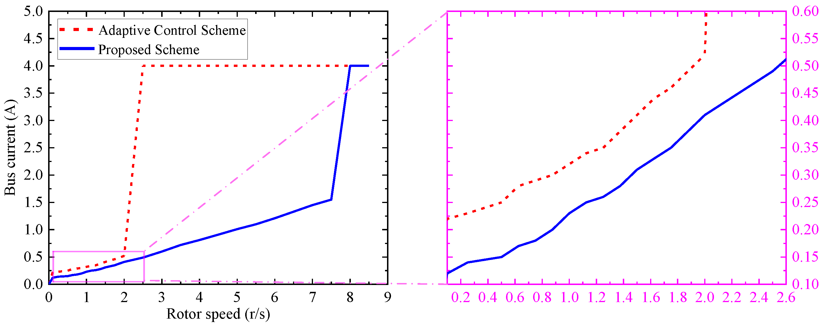
From Figure 9 and Figure 10, we conclude that the proposed scheme saves more on power consumption than the adaptive control scheme. To quantitatively study the power consumption of the motor under the stable operation, the steady current in the 28 $\mathrm{V}$ bus that supplies power to the two H-bridge circuits when accelerating from 0 to 8.5 $\mathrm{r}/\mathrm{s}$ in 18 $\mathrm{s}$ is shown in Figure 11. The desired operating speed is 2 $\mathrm{r}/\mathrm{s}$. At 2 $\mathrm{r}/\mathrm{s}$, the steady current $I_{AC}$$\left(\mathrm{A}\right)$ is about 0.52 $\mathrm{A}$ for the adaptive control scheme, and the steady current $I_{PC}$$\left(\mathrm{A}\right)$ is about 0.41 $\mathrm{A}$ for the proposed scheme. The bus voltage is denoted as $V_d$$\left(\mathrm{V}\right)$.

The power consumption $P_{AC}$ of the adaptive control scheme is approximately calculated as

$$P_{AC}=V_d{I}_{AC}\approx 14.56\mathrm{W}$$

(47)

The power consumption $P_{PC}$ of the proposed scheme can be approximately calculated as

$$P_{PC}=V_d{I}_{PC}\approx 11.48\mathrm{W}$$

(48)

Hence, the power consumption saving of the proposed scheme ${\eta }_{PC}$ is approximately computed as

$${\eta }_{PC}={\displaystyle \frac{P_{AC}-P_{PC}}{P_{AC}}}\approx {\displaystyle \frac{3.08}{14.56}}\approx 21.15\%$$

(49)

This energy-saving scheme, in addition to reducing the size of the power supply, can also

(1)

Extend in-orbit lifespan: Reduce battery consumption, prolong satellite operation time, and increase profit or scientific value.

(2)

Lower replacement costs: With extended battery life, fewer replacements are needed, reducing maintenance expenses.

(3)

Improve mission flexibility: Remaining power can be used for additional tasks or emergency situations, increasing the success rate of missions.

(4)

Simplify thermal management: Decreased heat generation simplifies cooling design, reducing complexity and cost.

(5)

Increase system redundancy: Less reliance on individual components enhances overall system reliability.

In summary, the long-term benefits include longer operational time, lower maintenance costs, higher mission success rates, and greater system reliability.

In the second experiment, two control schemes are used to implement the fixed point motion of the motor, respectively. If the motor runs at 0.1 $\mathrm{r}/\mathrm{s}$, the reference position ${\theta }_r$ (°) with respect to t$\left(\mathrm{s}\right)$ is expressed as

$${\theta }_r=\left\{\begin{array}{ccc}\hfill 36t& \hfill & \hfill 0\le t\le 3.6025\\ \hfill 129.69& \hfill & \hfill 3.6025<t\le 8.6025\\ \hfill 36\left(t-8.6025\right)+129.69& \hfill & \hfill 8.6025<t\le 11.0744\\ \hfill 218.68& \hfill & \hfill 11.0744<t\le 16.0744\\ \hfill 36\left(t-16.0744\right)+218.68& \hfill & \hfill 16.0744<t\le 18.6075\\ \hfill 309.87& \hfill & \hfill 18.6075<t\le 23.6075\\ \hfill 36\left(t-23.6075\right)+309.87& \hfill & \hfill 23.6075<t\le 25\\ \hfill 36\left(t-25\right)& \hfill & \hfill 25<t\le 26.0725\\ \hfill 38.61& \hfill & \hfill 26.0725<t\le 31.0725\end{array}\right.$$

(50)

When the four centers of the optical filters 1∼4 are collinear with the center of the light through the hole, respectively, the position of the filter wheel is $129.{69}^{\circ }$, $218.{68}^{\circ }$, $309.{87}^{\circ }$, and $38.{61}^{\circ }$, respectively. ${\theta }_r$ in Equation (50) is a trajectory used for sequential infrared radiation measurement of the four spectral segments. In Figure 12 and Figure 13, there are larger position errors when the filter wheel reaches the above four target positions for the adaptive control scheme. Moreover, the arrival index of ${\theta }_r$ in Equation (50) and that of the desired time for the filter wheel are poor. The filter wheel stays at the four target positions for 5 $\mathrm{s}$ for infrared radiation measurement, respectively. In fact, the infrared radiation measurement effect will begin to be affected when the position error is greater than or equal to $1.{44}^{\circ }$. For the adaptive control scheme, it is clear that the fixed point motion of the motor is not suitable for infrared radiation measurement. In Figure 12 and Figure 13, there are smaller position errors in the above four target positions for the proposed scheme. Moreover, the arrival index of ${\theta }_r$ in Equation (50) and that of the desired time for the filter wheel are good. It is clear that the fixed-point motion of the motor by the proposed scheme is suitable for infrared radiation measurement.

To test the position tracking performance of the proposed controller at higher speeds, the motor performs the fixed point motion at 0.2 $\mathrm{r}/\mathrm{s}$, 1 $\mathrm{r}/\mathrm{s}$, 2 $\mathrm{r}/\mathrm{s}$, 4 $\mathrm{r}/\mathrm{s}$, and 7.5 $\mathrm{r}/\mathrm{s}$, respectively. Their reference positions are all similar to ${\theta }_r$ in Equation (50). Their experimental results are shown in Figure 12 and Figure 13. When operating at 0.2 $\mathrm{r}/\mathrm{s}$, the performance of the adaptive control scheme is too poor to be used for infrared radiation measurement. The large current ripple prevents the motor from implementing the fixed point motion at 1 $\mathrm{r}/\mathrm{s}$, 2 $\mathrm{r}/\mathrm{s}$, 4 $\mathrm{r}/\mathrm{s}$, and 7.5 $\mathrm{r}/\mathrm{s}$ for the adaptive control scheme, respectively. Nevertheless, like 0.1 $\mathrm{r}/\mathrm{s}$, when operating at 0.2 $\mathrm{r}/\mathrm{s}$, 1 $\mathrm{r}/\mathrm{s}$, 2 $\mathrm{r}/\mathrm{s}$, 4 $\mathrm{r}/\mathrm{s}$, and 7.5 $\mathrm{r}/\mathrm{s}$, respectively, the position tracking performance of the proposed scheme is good enough to satisfy the infrared radiation measurement requirements.

In view of the characteristics of the space environment and the existence of severe vibration during the launch of the satellite, the temperature cycle experiment and vibration experiment are carried out successively. During the execution of the temperature cycle experiment, and after performing the vibration experiment, the previously described experiments need to be implemented once, respectively. It is shown that the experimental results are very close to those of the routine experiment. Therefore, the feasibility of the proposed scheme is further verified.

Finally,

Table 5. Scheme comparison.

Parameter	Paper [36]	Papers [34,35]	Paper [37]	This Work
Input Voltage $\left(\mathrm{Vdc}\right)$	28	28	28	28
Operation Mode	Constant Voltage Drive	Closed-loop Control	Constant Current Control	Constant Current Control
Implementation	System Level Design	System Level Design	System Level Design	Fully Integrated Design
Power Consumption $\left(\mathrm{W}\right)$	22.4@0.2 $\mathrm{r}/\mathrm{s}$	14.56@2 $\mathrm{r}/\mathrm{s}$	12.58@2 $\mathrm{r}/\mathrm{s}$	11.48@2 $\mathrm{r}/\mathrm{s}$
Current Ripple $\left(\mathrm{mA}\right)$	50@0.2 $\mathrm{r}/\mathrm{s}$	175@2 $\mathrm{r}/\mathrm{s}$	35@2 $\mathrm{r}/\mathrm{s}$	8@2 $\mathrm{r}/\mathrm{s}$
Load Capability	Poor	Poor	Good	Good
Steady Speed $\left(\mathrm{r}/\mathrm{s}\right)$	<0.3	<0.75	<3	<8
Tracking Error (°)	[0.89, 1.81]@0.2 $\mathrm{r}/\mathrm{s}$	[3.88, 4.46]@0.2 $\mathrm{r}/\mathrm{s}$	[0.09, 0.17]@0.2 $\mathrm{r}/\mathrm{s}$	[0.03, 0.08]@0.2 $\mathrm{r}/\mathrm{s}$

summarizes the main features of the proposed scheme in comparison with the adaptive control scheme [34,35], constant voltage drive [36], and the fuzzy logic method [37]. From Table 5, it can be observed that compared with existing solutions, the proposed scheme has advantages such as a fully integrated design, low power consumption, small current ripple, high load capability, the ability to achieve higher steady-state speed, and low tracking error. In conclusion, the designed driver has been proven to be effective and capable of adjusting the output current to achieve the desired speed when the load changes.

5. Conclusions

A SM driver designed for aerospace applications is presented. This driver utilizes a BPNN for reference current estimation and employs current subdivision for PWM signal generation. The driver’s hardware circuit design is detailed. The system dynamically adjusts drive current based on workload variations and maintains a stable bus current in the H-bridge circuit during periods of stable workload. This approach offers improved power efficiency compared to previous solutions. The entire control scheme, including rotor position angle measurement, two-phase current measurement, and BPNN-based current subdivision control, is implemented on a single FPGA. Experimental results demonstrate the effectiveness of the proposed driver.

Although the proposed method possesses a degree of universality, its practical application necessitates the consideration of motor parameter discrepancies, load inertia variations, and hardware resource constraints. Future research will focus on implementing parameter self-adaptive control, robust control techniques, and hardware optimization strategies to enhance the scheme’s generalization capabilities and extend its application range.

In view of the significance of numerical precision for practical applications, future work will focus on this issue, with specific research areas including the following:

(1)

Assessing the impact of different fixed-point bit-widths and quantization strategies on control accuracy.

(2)

Developing numerical error models and designing error compensation algorithms.

(3)

Proposing FPGA-implementable quantitative precision optimization schemes tailored to the specific characteristics of the control system.

Performance under varying loads or speed fluctuations is a worthwhile area for further investigation. Future work considers the following:

(1)

Varying the mass of the filter wheel, or using an adjustable inertia load, to simulate different load conditions.

(2)

Introducing external disturbances, such as simulating speed fluctuations, to test the robustness of the proposed control strategy.

Furthermore, future work will systematically evaluate the driver’s performance under various potential fault modes, explore fault-tolerance and degradation mechanisms, and propose corresponding optimization measures to enhance the system’s robustness and reliability.

It should be pointed out that the impact of total harmonic distortion (THD) on motor performance has been carefully considered. During the design process, an optimized PWM control strategy and output filtering circuits were adopted to reduce harmonics. Nevertheless, because the application prioritizes motor accuracy over efficiency, a fast current response was prioritized, and thus, requirements for THD were appropriately relaxed. Furthermore, due to the specific nature of aerospace applications, volume and weight constraints are considered key factors, and adding additional filter circuits would significantly increase the system’s volume and weight. Therefore, a compromise solution was chosen. In the future, reducing THD further while meeting volume and weight constraints will be researched through more advanced control algorithms or novel filtering technologies.

References

1. Sargos, F.M.; Zaskalicky, P.; Gudefin, E.J. Structures theory of reluctance step motors. IEEE Ind. Appl. Mag. 1995, 1, 28–32. [Google Scholar] [CrossRef]
2. Lee, K.M.; Kwan, C.K. Design concept development of a spherical stepper for robotic applications. IEEE Trans. Robot. Autom. 1991, 7, 175–181. [Google Scholar] [CrossRef]
3. Lyshevski, S.E. Electromechanical flight actuators for advanced flight vehicles. IEEE Trans. Aerosp. Electron. Syst. 1999, 35, 511–518. [Google Scholar] [CrossRef]
4. Condit, R.; Jones, D.W. Stepping Motors Fundamentals; Publication AN907; Microchip Inc.: Chandler, AZ, USA, 2004; pp. 1–22. [Google Scholar]
5. Aranjo, B.; Soori, P.K.; Talukder, P. Stepper motor drives for robotic applications. In Proceedings of the 2012 IEEE International Power Engineering and Optimization Conference, Melaka, Malaysia, 6–7 June 2012; pp. 361–366. [Google Scholar]
6. Kim, W.; Shin, D.; Chung, C.C. Microstepping with nonlinear torque modulation for permanent magnet stepper motors. IEEE Trans. Control Syst. Technol. 2012, 21, 1971–1979. [Google Scholar]
7. Le, K.M.; Van Hoang, H.; Jeon, J.W. An advanced closed-loop control to improve the performance of hybrid stepper motors. IEEE Trans. Power Electron. 2017, 32, 7244–7255. [Google Scholar] [CrossRef]
8. Bellini, A.; Concari, C.; Franceschini, G.; Toscani, A. Mixed-mode PWM for high-performance stepping motors. IEEE Trans. Ind. Electron. 2007, 54, 3167–3177. [Google Scholar] [CrossRef]
9. Kim, W.; Choi, I.; Chung, C.C. Microstepping with PI feedback and feedforward for permanent magnet stepper motors. In Proceedings of the 2009 ICCAS-SICE, Fukuoka, Japan, 18–21 August 2009; pp. 603–607. [Google Scholar]
10. Manea, S. Stepper Motor Control with dsPIC DSCs; Microchip Application Note; Microchip Inc.: Chandler, AZ, USA, 2009; pp. 1–26. [Google Scholar]
11. Kim, W.; Choi, I.; Bae, K.S.; Chung, C.C. A Lyapunov method in microstepping control for permanent magnet stepper motors. In Proceedings of the 2009 IEEE International Conference on Mechatronics, Málaga, Spain, 14–17 April 2009; pp. 1–5. [Google Scholar]
12. Kim, W.; Shin, D.; Chung, C.C. Microstepping using a disturbance observer and a variable structure controller for permanent-magnet stepper motors. IEEE Trans. Ind. Electron. 2012, 60, 2689–2699. [Google Scholar] [CrossRef]
13. Kim, W.; Shin, D.; Chung, C.C. The Lyapunov-based controller with a passive nonlinear observer to improve position tracking performance of microstepping in permanent magnet stepper motors. Automatica 2012, 48, 3064–3074. [Google Scholar] [CrossRef]
14. Gaan, D.R.; Kumar, M.; Sudhakar, S. Real-time precise position tracking with stepper motor using frequency modulation based microstepping. IEEE Trans. Ind. Appl. 2017, 54, 693–701. [Google Scholar] [CrossRef]
15. Schweid, S.A.; McInroy, J.E.; Lofthus, R.M. Closed loop low-velocity regulation of hybrid stepping motors amidst torque disturbances. IEEE Trans. Ind. Electron. 1995, 42, 316–324. [Google Scholar] [CrossRef]
16. Lee, Y.; Shin, D.; Kim, W.; Chung, C.C. Proximate in-phase current estimator to reduce torque ripple in permanent-magnet stepping motor. IEEE Trans. Ind. Electron. 2015, 63, 1707–1716. [Google Scholar] [CrossRef]
17. Yang, S.M.; Kuo, E.L. Damping a hybrid stepping motor with estimated position and velocity. IEEE Trans. Power Electron. 2003, 18, 880–887. [Google Scholar] [CrossRef]
18. Bose, B.K. Neural network applications in power electronics and motor drives—An introduction and perspective. IEEE Trans. Ind. Electron. 2007, 54, 14–33. [Google Scholar] [CrossRef]
19. Nguyen, T.T.; Tran, H.N.; Nguyen, T.H.; Jeon, J.W. Recurrent neural network-based robust adaptive model predictive speed control for PMSM with parameter mismatch. IEEE Trans. Ind. Electron. 2022, 70, 6219–6228. [Google Scholar] [CrossRef]
20. Mahfoud, S.; Derouich, A.; El Ouanjli, N.; el Mahfoud, M. Enhancement of the direct torque control by using artificial neuron network for a doubly fed induction motor. Intell. Syst. Appl. 2022, 13, 200060. [Google Scholar] [CrossRef]
21. Liu, Z.; Gao, H.; Yu, X.; Lin, W.; Qiu, J.; Rodríguez-Andina, J.J.; Qu, D. B-spline wavelet neural-network-based adaptive control for linear-motor-driven systems via a novel gradient descent algorithm. IEEE Trans. Ind. Electron. 2023, 71, 1896–1905. [Google Scholar] [CrossRef]
22. Li, Z. Robust control of PM spherical stepper motor based on neural networks. IEEE Trans. Ind. Electron. 2009, 56, 2945–2954. [Google Scholar]
23. Tran, H.N.; Le, K.M.; Jeon, J.W. Adaptive current controller based on neural network and double phase compensator for a stepper motor. IEEE Trans. Power Electron. 2018, 34, 8092–8103. [Google Scholar] [CrossRef]
24. Monmasson, E.; Cirstea, M.N. FPGA design methodology for industrial control systems—A review. IEEE Trans. Ind. Electron. 2007, 54, 1824–1842. [Google Scholar] [CrossRef]
25. Idkhajine, L.; Monmasson, E.; Naouar, M.W.; Prata, A.; Bouallaga, K. Fully integrated FPGA-based controller for synchronous motor drive. IEEE Trans. Ind. Electron. 2009, 56, 4006–4017. [Google Scholar] [CrossRef]
26. Muresan, C.I.; Folea, S.; Mois, G.; Dulf, E.H. Development and implementation of an FPGA based fractional order controller for a DC motor. Mechatronics 2013, 23, 798–804. [Google Scholar] [CrossRef]
27. Carfagna, E.; Migliazza, G.; Medici, M.; Lorenzani, E. Performance comparison between microstepping and field-oriented control for hybrid stepper motors. Energies 2025, 18, 1–14. [Google Scholar] [CrossRef]
28. Jaswal, A.; Abu-Ayyad, M.M.; Lad, Y.; Attaluri, A. Stepper motor position control using PD and MPC algorithms embedded in programmable logic controller. IEEE Access 2025, 13, 39096–39106. [Google Scholar] [CrossRef]
29. Daoudi, A.; Amrani, M.Z.; Achour, N. A novel stepper motor haptic interface for efficient robotic task programming. J. Eur. Syst. Autom. 2024, 57, 1369–1376. [Google Scholar] [CrossRef]
30. Jang, J.O. Neural network saturation compensation for DC motor systems. IEEE Trans. Ind. Electron. 2007, 54, 1763–1767. [Google Scholar] [CrossRef]
31. La Salle, J.; Lefschetz, S. Stability by Liapunov’s Direct Method with Applications; Academic Press: New York, NY, USA, 1961. [Google Scholar]
32. Hagan, M.T.; Demuth, H.B.; Beale, M. Neural Network Design; PWS Publishing Co.: Worcester, UK, 1997. [Google Scholar]
33. Baluta, G. Microstepping mode for stepper motor control. In Proceedings of the 2007 International Symposium on Signals, Circuits and Systems, Iasi, Romania, 13–14 July 2007; Volume 2, pp. 1–4. [Google Scholar]
34. Shi, X.; Iu, L.; Hang, S. Research for digital DC PWM controlling system. In Proceedings of the 2012 International Conference on Future Energy, Environment, and Materials, Energy Procedia, Hong Kong, China, 18–22 November 2012; Volume 16, pp. 1547–1552. [Google Scholar]
35. Chien, C.J.; Fu, L.C. Adaptive variable structure control. Adapt. Control Syst. 1999, 22, 41–62. [Google Scholar]
36. Morar, A. Unipolar fixed-current chopper—4 phase stepper motor driver system. Procedia Technol. 2014, 12, 75–82. [Google Scholar] [CrossRef]
37. Alfanz, R.; Fauzy, M.F.; Firmansyah, T. Error angle sun earth geometry analysis on fuzzy logic method in dual-axis solar tracking mounting design. In Proceedings of the 2024 FORTEI-International Conference on Electrical Engineering (FORTEI-ICEE), Badung, Indonesia, 24–25 October 2024; pp. 199–204. [Google Scholar]
Figure 1. Multispectral infrared image optical system in a satellite: (a) motion mechanism; (b) schematic diagram of the infrared image optical system.
Energies 18 03173 g001
Figure 2. Structure of the SM system.
Energies 18 03173 g002
Figure 3. Block diagram of the motor drive circuit.
Energies 18 03173 g003
Figure 4. Single phase drive circuit based on IR2110.
Energies 18 03173 g004
Figure 5. Single phase sampling current amplification circuit.
Energies 18 03173 g005
Figure 6. Experimental setup: (a) hardware circuit board of the driver; (b) motor and Hall sensor; (c) prototype appearance; (d) routine experiment; (e) temperature cycle experiment; (f) vibration experiment.
Energies 18 03173 g006
Figure 7. Data frame format.
Energies 18 03173 g007
Figure 8. Flowchart of the implementation of the proposed control scheme: (a) proposed controller; (b) training system structure block diagram.
Energies 18 03173 g008
Figure 9. The 28 V bus current when the motor accelerates from 0 to the target speed.
Energies 18 03173 g009
Figure 10. Phase current when running at 2 r / s and 7.5 r / s , respectively: (a) 2 r / s ; (b) 7.5 r / s .
Energies 18 03173 g010
Figure 11. Steady current in 28 V bus at different speeds.
Energies 18 03173 g011
Figure 12. Position and position error of the filter wheel when the motor runs at low speed.
Energies 18 03173 g012
Figure 13. Position and position error of the filter wheel when the motor runs at high speed.
Energies 18 03173 g013