1. Introduction
Global energy demand increased by 4.5% in 2021 and the global increase in energy demand also increased CO
2 emissions, according to the International Energy Agency (IEA). In 2023, the world is facing a global energy crisis, due to pandemic effects and the Russian invasion of Ukraine, of unprecedented depth and complexity [
1]. Therefore, in the coming years, it will be important to substitute much of the energy produced from natural gas with energy from other energy sources.
Renewable energy systems can serve this purpose and, at the same time, are able to mitigate the growth of the global environmental problem of CO2 emissions. Solar and wind power are estimated to contribute to two thirds of the growth of renewables. These renewable sources are intermittent. However, considering their intermittence and the need to ensure an appropriate balance between energy production and energy demand, energy accumulation systems are necessary. Thermal storage systems are considered the most realistic and effective choice for this task due to their great potential in terms of energy management optimization and energy losses control.
Concentrating Solar Power (CSP) technologies are a key component in the transition to sustainable and dispatchable electricity generation, particularly in regions with high direct normal irradiance (DNI) [
2]. CSP systems use mirrors or lenses to focus sunlight onto a thermal receiver, where the energy is captured by a heat transfer fluid (HTF) and subsequently converted to electricity through a thermodynamic cycle. Among the four principal CSP configurations—parabolic trough, central tower, linear Fresnel, and dish-Stirling—the parabolic trough collector (PTC) remains the most commercially mature and extensively deployed worldwide [
3,
4].
Parabolic trough systems employ curved, mirrored surfaces to concentrate solar radiation onto a receiver tube located at the focal line of the parabola. Traditionally, synthetic thermal oils have been used as HTFs due to their favourable thermal stability in the 300–400 °C range. However, in recent years, molten salts have gained prominence as a heat transfer and storage medium due to their superior thermal stability at higher temperatures (typically 290–565 °C), lower vapor pressures, and compatibility with thermal energy storage (TES) systems [
5,
6]. This enables both improved thermodynamic efficiency and greater dispatchability of the power plant.
Integrating molten salt in parabolic trough systems introduces additional modelling complexity, as the salt’s thermophysical properties (e.g., specific heat, thermal conductivity, viscosity) vary significantly with temperature and affect heat transfer dynamics within the receiver tube. Moreover, salts such as a binary mixture of sodium nitrate and potassium nitrate (commonly known as Solar Salt 60% NaNO3–40% KNO3) require specific handling to avoid freezing and ensure proper startup/shutdown procedures. Accurate thermal modelling, therefore, becomes essential for system design, control, and optimization.
Many mathematical models, analytical and numerical, have been developed in order to simulate the heat transfer phenomena and improve the thermal performance of PTCs.
Analytical models offer the advantages of simple and fast computation of the main thermal variables in a plant, but if the purpose of thermal analysis is to know a point temperature distribution over the entire domain of a component, a numerical model that offers the possibility of simulating detailed geometric configurations also with complex conditions is necessary, such as the FEM model presented in [
7] or the FVM model presented in [
8].
Ratzel et al. [
9] carried out both analytical and numerical studies of the heat conduction and convective losses in an annular receiver for different geometries. Dudley et al. [
10] developed an analytical model of an SEGS LS-2 parabolic solar collector, with synthetic oil as HTF, considering the heat collector element in a one-dimensional steady state: the model was validated with experimental data for different receiver annulus conditions: vacuum intact, lost vacuum (air in annulus), and also bare tube.
The Forristall model, developed at the National Renewable Energy Laboratory (NREL), is widely used to simulate thermal losses from the receiver tube and remains a benchmark for simulation of parabolic trough collectors [
11]. This model provides a basis for assessing system performance under variable operating conditions. However, real-world operation often deviates from idealized assumptions due to optical degradation, tracking errors, ambient wind effects, and unsteady thermal loads [
12,
13].
To bridge this gap, recent studies have focused on validating simulation models against field data. Li et al. [
14] improved thermal loss modelling to better replicate transient performance under fluctuating irradiance, while Surrender et al. [
15] explored the impact of different HTFs, including molten salt, on collector efficiency.
This paper presents a detailed analysis of a parabolic trough solar thermal system operating with molten salt as HTF, comparing experimental data from plant operation with the results of a simulation model incorporating the Forristall thermal loss formulation. The study aims to evaluate the accuracy of the model in replicating real system behaviour, quantify deviations under different solar and thermal loads, and provide insights for improving CSP plant modelling with advanced HTFs.
2. Enea PCS Plant Description
In the period 2001–2010, ENEA, after an initial exploratory phase, developed an innovative concept of a CSP plant using molten salts as the heat transfer fluid in a linear parabolic system. The chosen concept, the use of molten salts as medium of heat transfer fluid and as a fluid thermal storage, is called “direct accumulation”, and it was used initially in tower systems (e.g., Solar Two in the US), where it is still applied. Traditionally, linear parabolic systems employed diathermic oil as a heat transfer fluid and molten salts as storage fluids; this technique is called “indirect accumulation”, and it was widely used in the Andasol-type Spanish plants.
Indirect accumulation has a few relevant disadvantages: it requires the use of heat exchangers between the two fluids, which add cost and complexity and involve a decrease in performance; accumulation is limited and is not very effective, as the maximum oil temperature (400 °C) also limits the maximum salt temperature. Where classic molten salts are used as the accumulation system, this implies that the interval of usable temperature, in an indirect system, is reduced to 100 °C (between 290 and 390 °C) against 260 °C (between 290 and 550 °C) in comparation to direct systems.
The use of molten salt as a heat transfer fluid (HTF) in parabolic linear systems required a series of technological developments for the key components of the CSP plant, such as solar collectors, receiver tubes, and the thermal storage system.
These new components and systems have been developed and patented by ENEA, after being tested under real operating conditions in the test facility (PCS plant) completed in 2003 at the ENEA Casaccia research centre [
16,
17]. The PCS plant allows researchers to carry out tests in real operational conditions and test components of solar power systems. The facility is still in operation and continues to serve as a valuable experimental platform, where periodic upgrades and improvements are implemented to incorporate the latest technological advances. Of particular importance in the innovation efforts undertaken by ENEA are the receiver tubes, which are capable of operating at 550 °C thanks to a specially developed coating designed to maximize solar energy absorption while minimizing heat losses by radiation.
Another notable aspect was the development and engineering of an auxiliary heating pipe system, necessary to guarantee the preheating of the lines before start-up filling with hot salts and keep the pipe system under working temperature in case of operations abnormalities or maintenance. Heating systems of solar receiver (Heat Collector Element, HCE) tubes, due to their engineering innovations with glass vacuum cavities, do not allow the use of traditional heating methods (such as electrical tracing), but use the Joule effect.
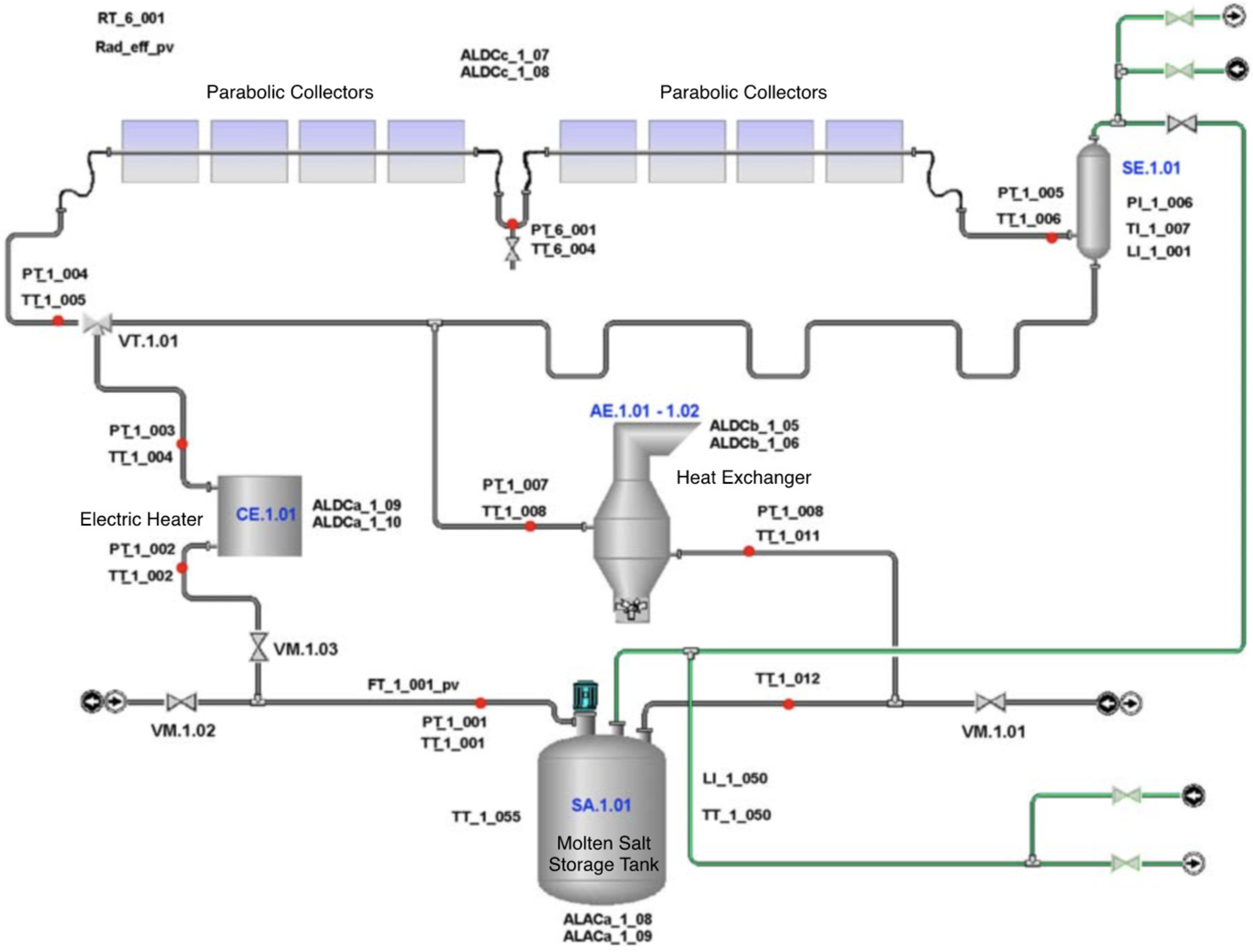
The PCS plant, shown schematically in
Figure 1, consists of the test section (the solar collector with the receiver tube), the storage tank (SA.1.01) with the circulation pump, the connecting pipes, an electric salt heater (CE.1.01), and a heat exchanger (AE.1.01–AE.1.02). The test section of the plant consists of two linear parabolic trough collectors, oriented in an East–West direction, with an opening of about 6 m and a length of about 50 m (the Solar Collector Assemblies (SCA) in total is about 100 m long), equipped with a hydraulic piston system for handling. Due to the Solar Salt’s high melting temperature, all plant components are properly insulated to minimize heat losses and are heated either with external electric cable (storage tank, piping, valve, flanges, instruments) or by direct Joule effect (the receiver tube, HCE).
During operation, the fluid is kept in motion inside the circuit pipes by a vertical-axis centrifugal pump located inside the storage tank. The flow rate can be adjusted by varying the pump speed within an inverter. Under normal operating conditions, a flow rate is maintained of around 6.2 kg/s.
The electric heater has the purpose of regulating the temperature and maintaining the required temperature of the HTF entering the solar field. In the receiver tube, the HTF, depending on the intensity of solar radiation, heats up by absorbing solar energy reflected and concentrated by the parabolic mirrors, then the fluid passes through the heat exchanger (HE), which has the function of removing the heat provided by solar radiation, and then returns to the storage tank at the desired temperature. A series of experimental tests have been conducted on the PCS plant to characterize both the behaviour of different heat transfer fluids and the optical, thermal, and mechanical performance of the main components of the solar system, in particular, the two main components of a solar plant: the linear parabolic collector and the receiver tube (HCE). Both these components were designed and developed by ENEA. Based on the theoretical concepts developed by ENEA on molten salts and the experimental tests conducted on the PCS plant, experimental test facilities were developed to validate the components of molten salt technology [
18]; in addition, a 1 MWe demonstration plant was completed in Egypt in 2019 [
19].
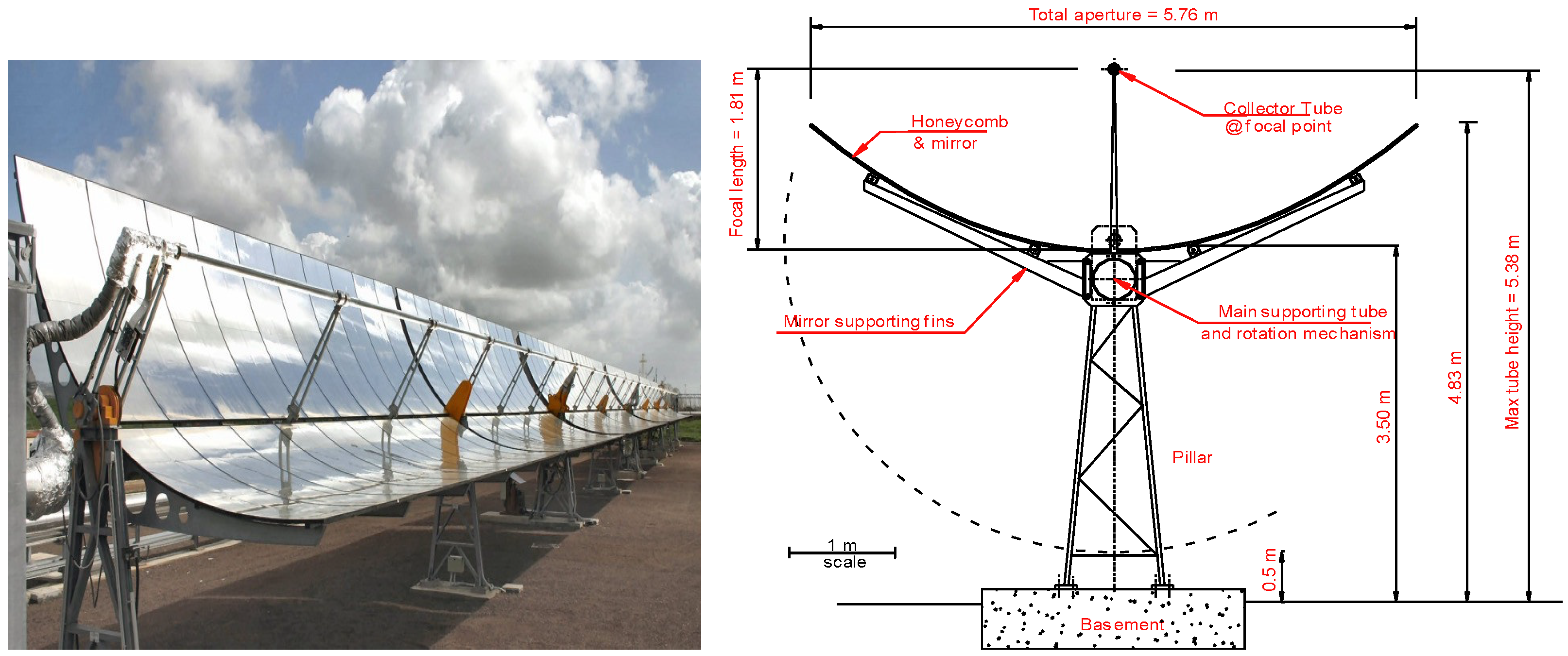
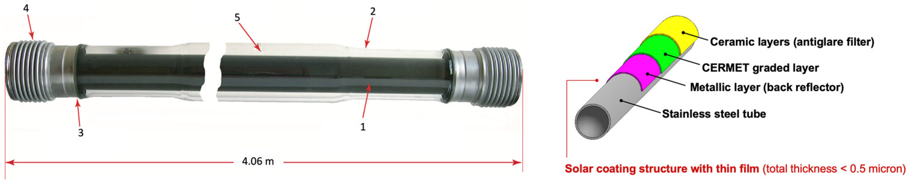
Figure 2 shows, on the left, a photo and, on the right, a technical drawing of the solar collector of the PCS plant.
In
Table 1, the main data of the PCS solar field are summarized.
Throughout an experimental test the data acquisition system can acquire up to 83 quantities over the entire plant with acquisition start/stop times of 7 a.m. and 9 p.m. and a sampling time of 5 s.
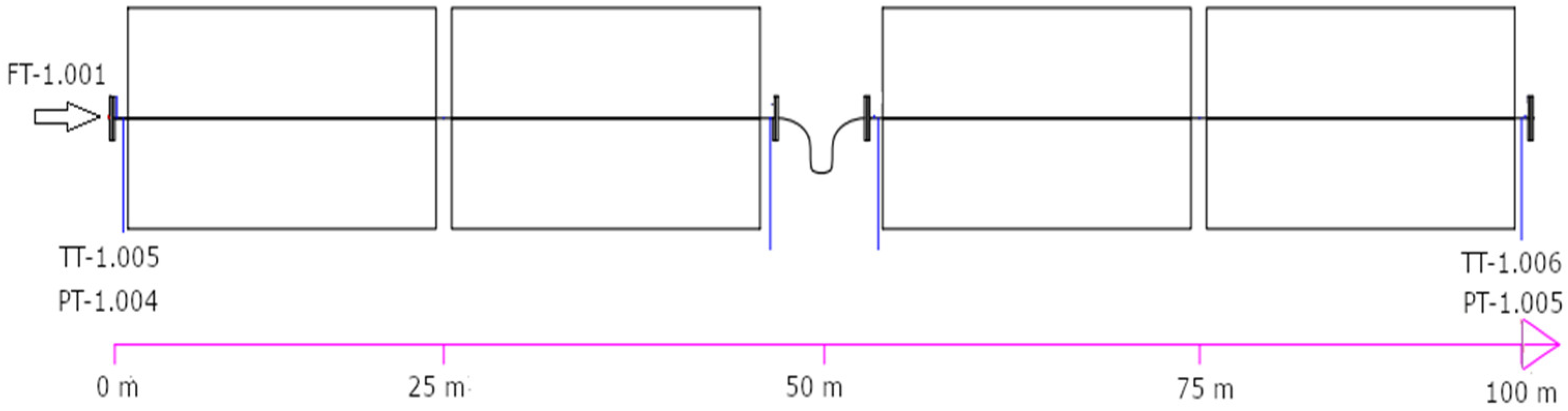
Figure 3 shows a scheme of the test section (SCA) of the plant with an indication of the main acquired quantities on the collector.
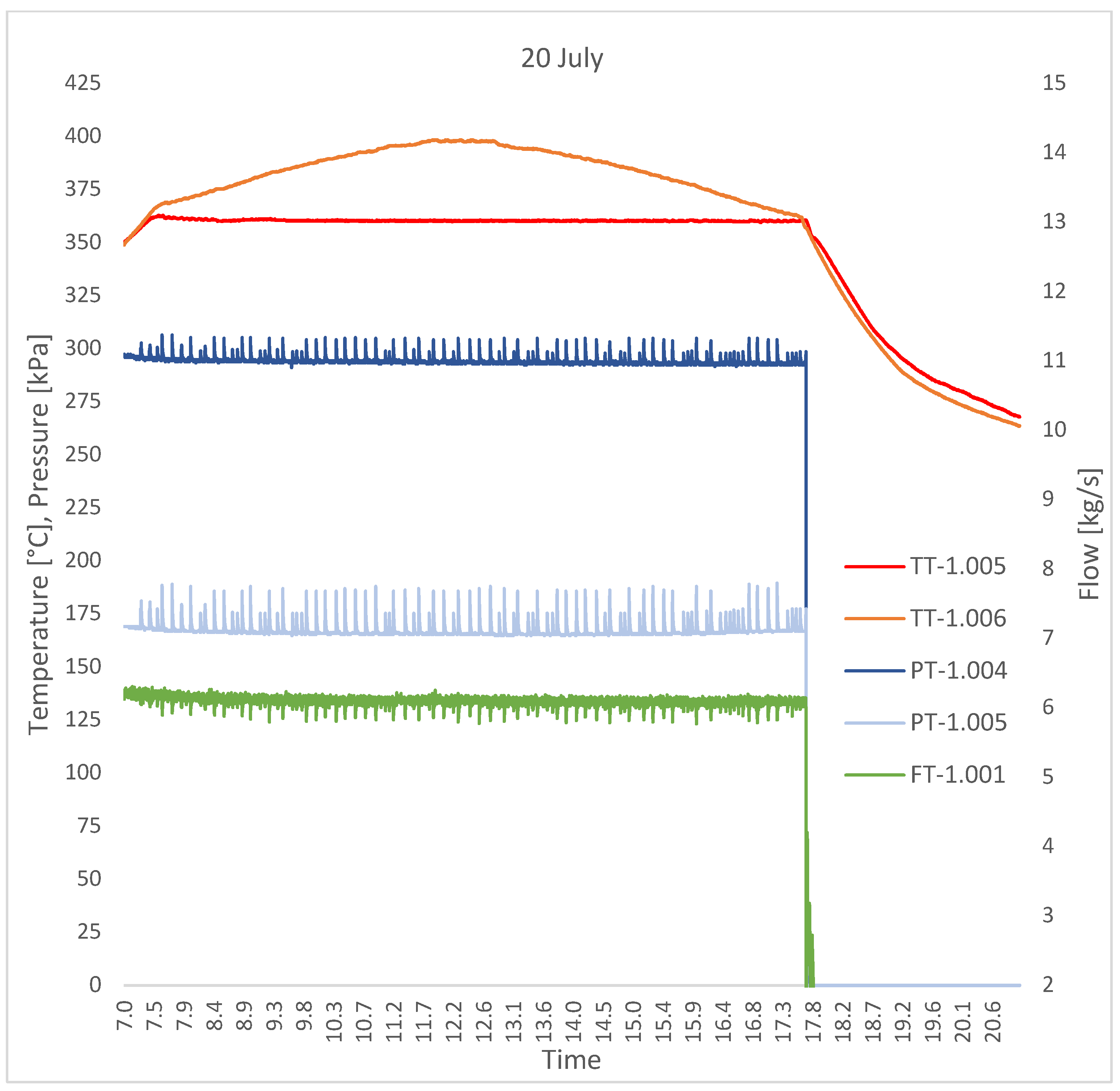
Figure 4 shows the trends of the HTF main acquired measured quantities in the experimental test carried out on 20 July.
Therefore, the measured quantities shown in
Figure 3 and
Figure 4 are the HTF flow rate (FT-1.001), temperatures (TT-1.005, TT-1.006), and pressure (PT-1.004, PT-1.005) of the HTF at the inlet and outlet of the receiver tube. These five variables, together with direct normal irradiance, RT-6.001, ambient temperature, TT-6.009, and local wind speed, ST-6.001, are summarized in
Table 2.
The flow rate and the temperatures at the inlet and outlet of the solar collector are the quantities related to the heat transfer fluid needed to calculate the thermal power (PHTF).
Heat fluxes related to the solar collector and the receiver are referred to schematically in
Figure 5, where P
HTF is the thermal power transferred to the fluid considering the power loss due to the optical and thermal efficiencies of the system, P
LOSS; P
SUN is the solar power that impacts on the collector; and P
HCE is the power intercepted by the receiver tube.
Next, having acquired values of the temperatures at the inlet and outlet of the receiver tube, it is possible to calculate the thermal power transferred to the fluid, P
HTF, with Equation (1).
The physical properties for the working fluid used in the experimental tests (Solar Salt, NaNO
3/KNO
3, 60:40 wt.%) are summarized in
Table 3.
The solar power, P
SUN, referring to
Table 1, can be calculated as
where L
act is the active length of the total receiver tubes. L
act can be calculated with Equation (3), with the considered quantities N
HCE, L
HCE, and L
soff indicated in
Table 4.
DNIEFF is the effective direct radiation, calculated by multiplying the direct radiation by the cosine of the angle of incidence.
Therefore, having P
SUN and P
HTF, it is possible to calculate the global solar field efficiency with Equation (4)
Over the years, various collectors and receiver tubes have been used in the PCS solar field, either to test their different characteristics or simply to replace old types with new generations of HCEs and/or mirrors. Generally, the solar receiver used in systems with linear parabolic concentrators is a metal tube (absorber tube) encapsulated in a glass tube whose function is to reduce thermal losses. The glass used can reduce thermal convection losses (wind effect) but also thermal radiation because glass is mostly opaque in the infrared irradiation field. To ensure a high degree of thermal insulation of the receiver, the annular cavity between the absorber tube and the glass tube is under vacuum pressure (10−2 Pa). The surface of the absorber tube is coated with a selective coating, characterized by a high absorption coefficient and low emissivity in the infrared radiation range, so the coating significantly affects the efficiency of the receiver.
ENEA has been working for several years on the development of selective coatings that are stable at high temperatures in vacuum conditions for CSP applications. The work has focused on multilayer coatings composed of a low-emissivity metallic layer, a CERMET layer. This is a composite material made of ceramic and metallic particles that ensures a high absorption of visible radiation and is ultimately an external anti-reflection layer [
20].
Table 4 shows the main properties of the two different types of receiver tubes used in the PCS system examined in this study.
In
Figure 6, tube #1, a receiver tube type patented by ENEA [
21], is schematically represented.
From a hydraulic point of view, a total pressure loss of approximately 130 kPa was measured during the experimental tests (
Figure 4). It should be emphasized that a large part of this loss was due to the flexible hoses (2″, internal diameter 55 mm) located at the inlet and outlet of each of the two external line collectors. In general terms, during the tests, a unit pressure loss of approximately 4 kPa/m was measured in the flexible hoses, while a pressure loss of approximately 0.35 kPa/m was estimated in the receiver tube.
3. Heat Transfer Model Description
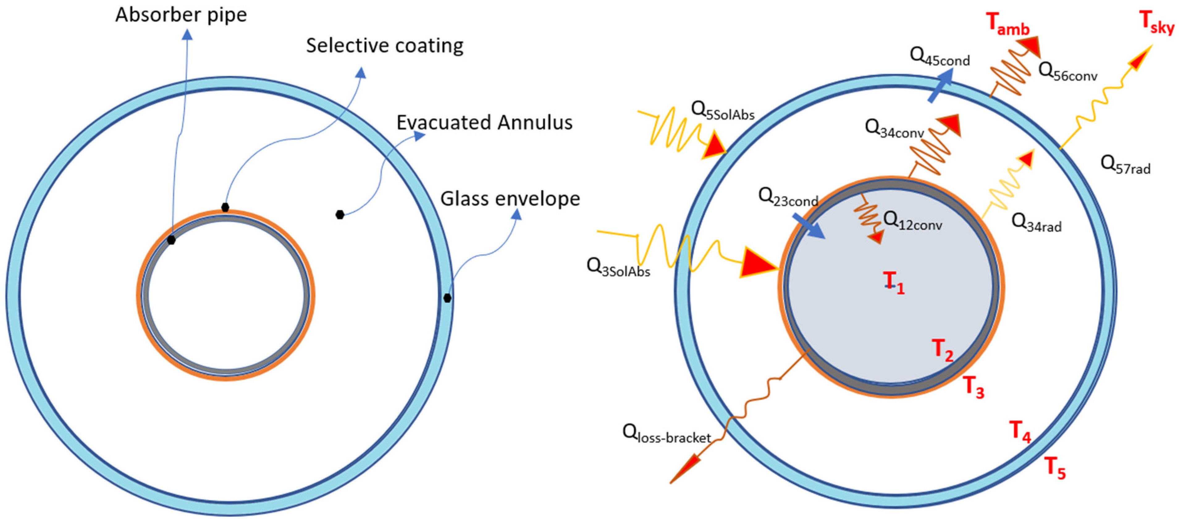
In this section, the description of the receiver tube’s mathematical heat balance model is presented. The receiver tube, heated by the radiant energy of the sun, is isolated from the external environment by the glass envelope and disperses heat towards the glass envelope by natural convection, by radiation, and by conduction through the metal supports that hold the tube on the structure. The glass envelope, which creates a quasi-vacuum cavity, is exposed to the ambient air, Tamb, and to ambient wind speed. The glass envelope disperses heat towards the external environment by forced convection and by radiation towards the sky (sky temperature, Tsky).
Figure 7 shows a cross-section of the solar receiver tube with indication of its different constituent parts (
Figure 7, left), and a simplified radial energy balance with indication of the heat fluxes (by conduction, convection, and radiation) and solar absorptions by radiation on the metallic tube and on the glass envelope (
Figure 7, right).
Relevant to the right side of
Figure 7, the solar energy reflected by the mirrors is absorbed by the glass envelope, Q
5SolAbs, and by the metallic absorber surface, Q
3SolAbs. A part of the energy absorbed into the metal is first conducted, Q
23cond, through the metal and then transferred to the HTF by forced convection, Q
12conv; remaining energy is transferred back to the glass envelope by radiation, Q
34rad, and natural convection, Q
34conv, and part of it lost through the support brackets by conduction, Q
cond-bracket. The heat loss coming from the absorber (radiation and natural convection) passes through the glass envelope by conduction, Q
45cond, and, along with the energy absorbed by the glass envelope, is lost to the environment by convection, Q
56conv, and to sky by radiation, Q
57rad. The purpose of the mathematical energy balance model is therefore to simulate, under stationary conditions, the behaviour of a HTF entering the pipe at a certain known temperature, T
in, and leaving the pipe at a temperature, T
out_sim, which needs to be calculated. Obviously, the outlet temperature, T
out, is acquired in the experimental tests and thus it is possible to compare the real acquired results with the results obtained with the simulations.
When the type and the optical properties of the collector and the HCE are considered, the mathematical expression for the absorbed energies on the absorber tube and glass envelope can be written as:
where Q
si is the solar irradiance per receiver unit length and can be calculated by multiplying the DNI by projected aperture area and dividing by total receiver length, η
env is the effective optical efficiency at the glass envelope expressed in Equation (7), and η
abs is the effective optical efficiency at the absorber expressed in Equation (8).
The parameter values used in the code for all the terms in Equations (5)–(7) are summarized in
Table 5.
The convection heat fluxes from the inner surface of the absorber tube to the fluid, Q
12conv, between the external metal surface of the absorber and the glass envelope, Q
34conv, and from the glass envelope to the ambient atmosphere, Q
56conv, can be derived from Newton’s law:
where
,
, and
are, respectively, the convection heat transfer coefficients for the fluid, the annulus gas, and the ambient air;
,
, and
are, respectively, the inside and outside absorber tube diameters and glass envelope outer diameter; and
are, respectively, the mean HTF temperature, inside and outside surface temperatures of the absorber pipe, inside and outside surface temperatures of the glass envelope, and ambient temperature. Heat transfer coefficient
is calculated at
; the coefficients
are calculated at mean temperature
. The convection heat flux for the annulus gas is calculated by free-molecular convection correlations when the annulus is under vacuum. Conversely, in the case when the annulus loses vacuum, in addition to the convection heat exchange, advection is also presented, and in this case the Raithby and Holland correlation can be used (natural convection between two concentric horizontal cylinders). The convection heat transfer from the glass envelope to the ambient is considered natural or forced convection depending on the presence or absence of wind. In the absence of wind (natural convection), the correlation developed by Churchill and Chu is used, while in the presence of wind, Zukauskas’s correlation [
22] is used.
The conduction heat fluxes through the absorber tube
and through the glass envelope
can be derived, in general, from Fourier’s law:
where
are the heat conduction coefficients for the absorber and for the glass envelope calculated at average absorber or glass envelope temperatures, (
Ti +
Tj)/
2;
are, respectively, inside and outside absorber and glass envelope diameters and temperatures.
The heat flux dispersed by conduction through the support brackets that link the receiver tube to the collector structure is calculated as:
where
is the average convection coefficient of the bracket,
is the perimeter of the bracket support,
is the conduction coefficient,
is the minimum cross-sectional area of the bracket,
is temperature at the base of the bracket,
is the ambient temperature, and
is the HCE length.
Figure 8 presents a picture of the brackets used on the experimental collector.
Here, it should be emphasized that the contribution to heat loss of the supports is limited and could, in a first approximation, be neglected.
The two radiation heat fluxes between the absorber and the glass envelope,
, and between the glass envelope and the sky,
, are:
where
is the Stefan–Boltzmann constant and
is the emissivities of the different surfaces.
Forristall has developed a two-dimensional model that describes the steady-state thermal behaviour of a linear receiver for parabolic trough systems [
9]. To implement this mathematical model, the receiver tube is divided along its length into N equal segments, with the assumption that temperature remains continuous at the boundaries between adjacent segments and that radial heat fluxes are normal and uniform to the surfaces in each segment, and the fluxes are calculated at the average temperature between the left and right edges of the segment. Additionally, only the thermal fluid is considered to transfer energy longitudinally, and the thermal conductivity is assumed to be constant. Based on the Forristall approach, a code software, written in C#, including all necessary equations and empirical relationships from Equation (5) to (14), has been implemented.
The energy balance, considering a single receiver tube segment, can be written as:
where
is
(solar absorption minus heat loss),
is the circumferential area of segment i,
is the fluid mass flow rate,
is the enthalpy, and
is the bulk fluid velocity.
The net heat flux is equal to the heat absorbed minus the heat loss:
where the solar absorption term,
, is the sum of the solar absorption in the glass envelope and in the absorber tube and they can be calculated with the Equations (4) and (5).
When we consider the active length of the receiver tubes, , whose value is calculated with Equation (2), we can calculate the receiver tube length with .
Now, when
is known, we can find the solar absorption term and the heat loss for each N receiver segment with Equations (17) and (18)
Assuming that fluid density is only a function of temperature, the enthalpy change in Equation (15) can be approximated by , where and, by substituting the above relations, Equations (16) and (18) in Equation (15), we can derive the considered temperature at the outlet receiver tube segment, .
The software calculation starts by considering the geographical coordinates and the time zone of the location in question (Enea Casaccia: latitude = 42.0499, longitude = 12.3055, time zone = GMT + 1), the date, and the ambient conditions from the weather location. With these input data, instant by instant, during the experimental test, it is possible to calculate solar angles (Azimuth and Zenith) throughout the duration of the experimental test. Solar angles are calculated using a sun position algorithm and, in the code, the routine developed by Grena [
23] is used. With the two solar angles, the model permits the calculation of the incidence angle, θ, which is the angle between the direction of the sun’s rays on the collector surface and the plane normal to that surface. This angle of incidence varies during the day (and of course during the year) and has a large influence on the collector’s performance.
Incidence angle for a single axis tracking aperture collector oriented in an East–West direction is given by:
where
is the solar elevation angle and A
Z is the solar azimuth angle.
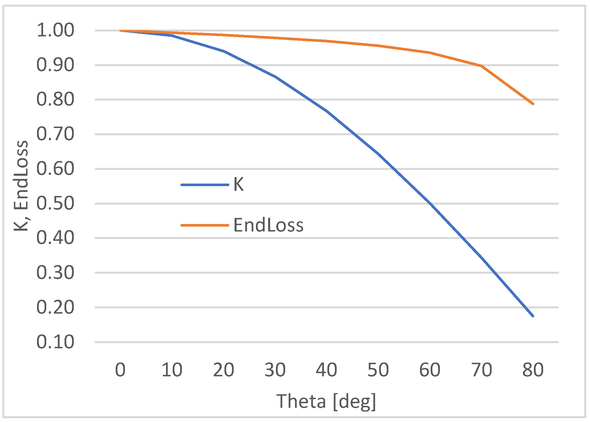
The solar collector losses that occur due to reflection and absorption by the glass envelope increase as the incident angle increases. The incidence angle modifier, K, corrects for these additional losses. Usually, the incidence angle modifier is provided as an empirical fit to experimental data for a given collector type. The solar collectors of the PCS plant are collectors designed by ENEA and, based on the performance tests conducted on the PCS plant, the incidence angle modifier can be expressed with the following formula:
The last considered performance parameter in the calculation is the geometric factor called the collector geometrical end losses (EndLoss factor). Terminal losses occur at the ends of the HCE: for a non-zero angle of incidence, a certain length of the absorber tube is not illuminated by the solar radiation reflected by the mirrors. The terminal losses are a function of the focal length of the collector, the collector length, and the angle of incidence. In the considered model, the terminal losses are expressed according to the following equation:
In Equation (21), f is the focal length of the collector and LSCA is the length of the solar collector.
In
Figure 9, the trend of the incidence angle modifier, K, and Endloss versus the incidence angle θ are shown.
The two coefficients, K and EndLoss, both functions of the incidence angle, θ, are the last two factors required to calculate and in Equation (6).
The code needs, as input, not only the described optical, geometrical, and thermal parameters, but also the temperature values of both the absorber tube, T2, and the glass envelope, T4, to be set as first attempt values. These values must then be as close as possible to the expected values in order to achieve convergence in a reasonable number of steps. In the code, a calculation loop is set up in which the losses are calculated and, once the results are obtained, the code performs a comparison of the heat exchange values between the absorber tube and the glass envelope and between the glass envelope and the external environment. If these two values are, within a certain limit, similar, the calculation proceeds; otherwise, the attempt values for the two temperatures are changed and the calculation is restarted.
4. Results and Discussion
As mentioned, the two tests were conducted with two different receiver tubes: tube #1 for the test on 20 July and tube #2 for the test on 2 September. The duration of each test and the range values of the six acquired parameters required for the analysis are summarized in
Table 6.
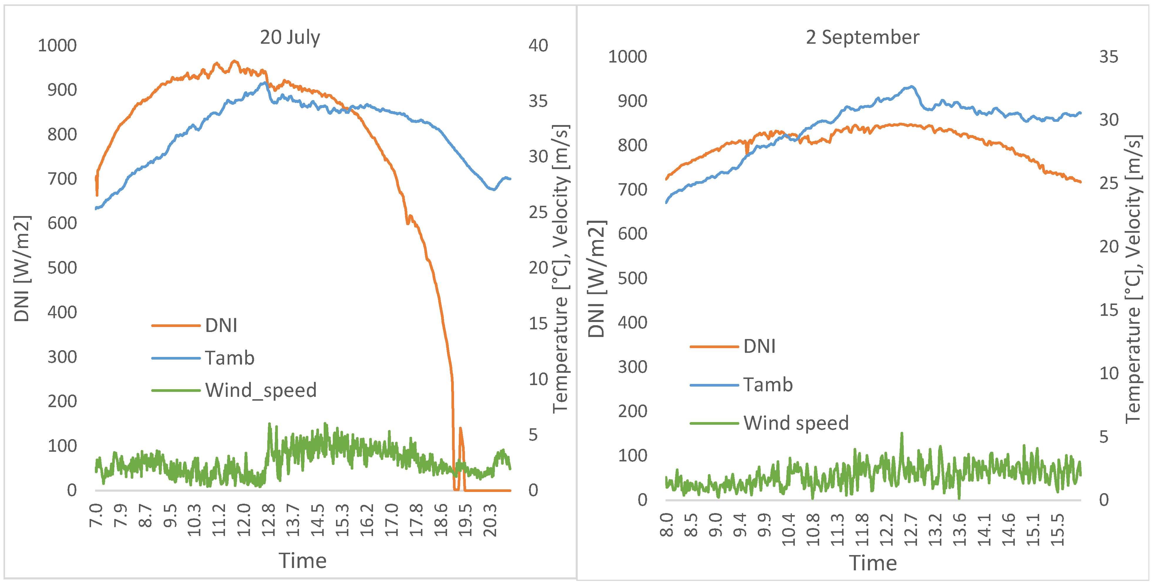
Figure 10 shows the trends of the measured meteorological variables, direct normal irradiation (DNI), ambient temperature (T
amb), and wind speed on minute resolution during the experimental tests of 20 July and 2 September.
The two days chosen for the comparison present a good solar radiation curve without significant changes due to sparse cloud conditions (almost clear sky) and air temperatures and wind speed conditions typical of the locations for the season of the year.
In
Figure 10,
Figure 11 and
Figure 12, the performance plant parameters calculated with the presented model are shown in comparison with the parameters acquired during the experimental runs.
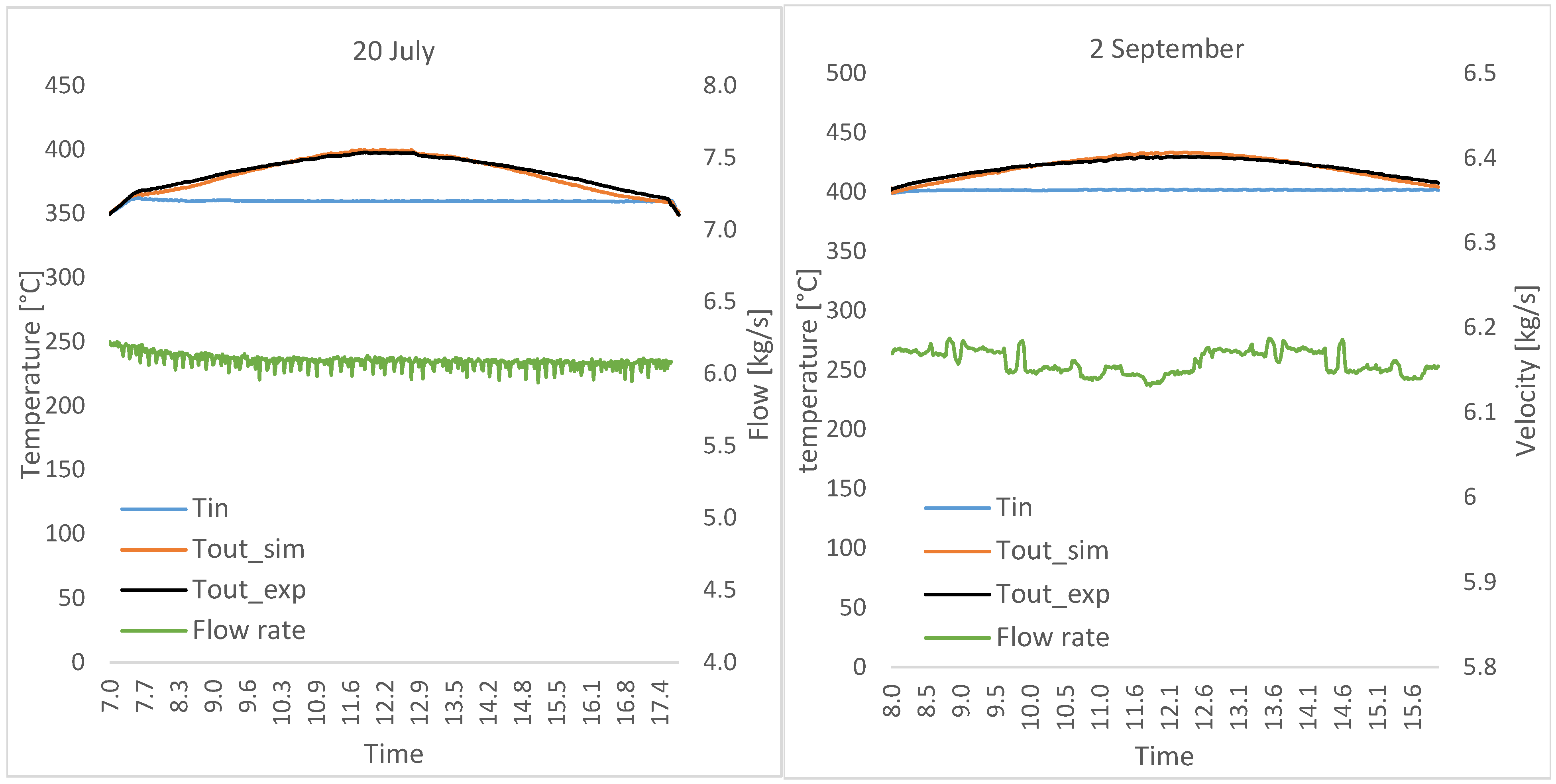
Figure 11 shows the acquired values of flow rate, inlet, and outlet temperature of the working fluid (Flow rate, T
in, and T
out_exp) and the outlet temperature of the fluid calculated with the simulation model (T
out_sim) for both test days. The subscript “exp” refers to the experiment, while “sim” refers to simulation values.
The average value of the temperature at the inlet of the tube in the test of 20 July is around 360 °C, while for 2 September the average value at the inlet is around 400 °C. The average value of the flow rate is around 6.1 kg/s in both tests. As can be seen from the graphs in
Figure 11, the measured and simulated values of the output temperatures, T
out_exp and T
out_sim, are very close and the maximum temperature rise is about 40 °C for the 20 July test and around 30 °C for the 2 September test.
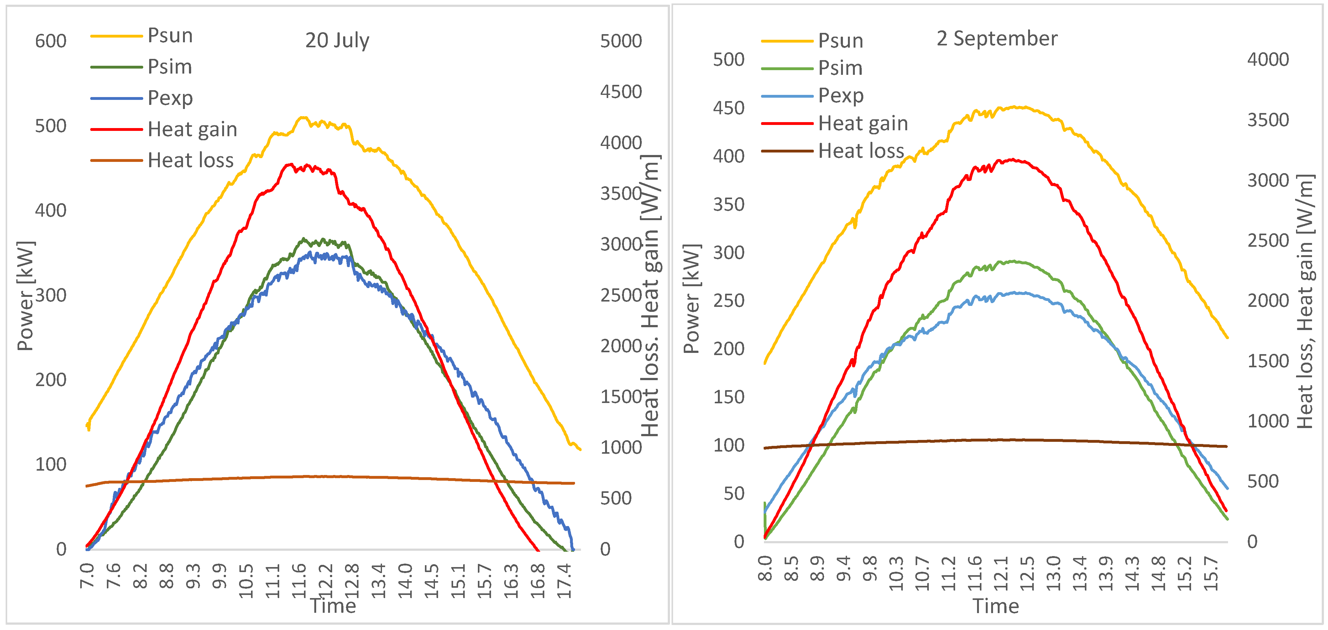
Figure 12 shows the solar power, P
sun, the HTF power, P
exp, the simulated HTF power, P
sim, Heat
gain, and Heat
loss for the 20 July test simulation (left) and (right) the 2 September test, respectively. The values found for Heatgain and Heatloss, refer to the unit length of the tube, and have an order of magnitude comparable with the values found for similar concentrating plants.
For a final comparison between the experimental and simulated data, it was decided to compare the global solar field efficiencies calculated with Equation (4), where the outlet temperature is the T
out_exp measured with the experiment and T
out_sim calculated with the model.
Figure 13 shows the global efficiencies and the incidence angle for the experimental test of 20 July (left) and 2 September (right).
The results of the comparison are summarized in
Table 7. In order to highlight the maximum difference between the values of the experimental and simulated efficiencies at different times of the day, the table shows the values of the variables at three different times during the experimental tests, that is, a value in the morning, a value in the afternoon, and a value referring to the instant when the angle of incidence assumes its minimum value, which, for the test of 20 July was at 12:16 and for the test of 2 September was at 12:09.
The Root Mean Square Error (RMSE, Equation (22)) is a key performance metric used to evaluate the accuracy of thermal models by quantifying the deviation between predicted and experimental temperature data. It is defined as the square root of the average of the squared differences between the measured temperatures and those predicted by the model:
where
Oi denotes the experimentally measured temperature at the i-th time T
out-exp,
Pi is the corresponding model-predicted temperature T
out-sim, and
n is the total number of data points. RMSE is expressed in the same units as temperature (°C), allowing for direct physical interpretation. In thermal analysis, a low RMSE indicates that the model reliably captures the heat transfer processes and boundary conditions governing the system.
In the last two columns of
Table 7, the difference between the two efficiencies and the value of the RMSE calculated for the temperature at the exit of the receiver tube for the simulated data and for the experimental data are shown. The RMSE values found, 2.92 and 2.61, indicate that the simulation results fit the acquired data very well, for both test days.


