Systemic Scaling of Powertrain Models with Youla and H_∞ Driver Control

Abstract

This paper presents a methodology for systematically scaling vehicle powertrain and other models and an approach for using model parameters and scaling variables to perform controller design. The parameter scaling method allows for high degrees of scaling while maintaining the target performance metrics, such as vehicle speed tracking, with minimal changes to the model code by the researcher. A comparison of proportional-integral, Youla parameterization, ${\mathrm{\text{H}}}_{\infty }$, and hybrid Youla-${\mathrm{H}}_{\infty }$ controllers is provided, along with the respective methods for maintaining controller performance metrics across degrees of model scaling factors. The application of the scaling and various control design methods to an existing model of a hydrogen fuel cell and a battery electric vehicle powertrain allows for the development of a representative scale model to be compared with experimental data generated by an actual scale vehicle. The comparison between scaled simulation and experimental data will eventually be used to inform the expected performance of the full-size electric vehicle based on full-size simulation results.

1. Introduction

Previous work on the development of a model for hydrogen proton-exchange membrane fuel cells (PEMFC) [1] and on electric vehicle (EV) powertrains [1] resulted in a detailed simulation to be used for evaluating energy management strategies between the PEMFC and the battery during the execution of various drive cycles.

This prior work is important in supporting the exploration of alternative energy systems for transportation. Higher efficiency energy management strategies contribute towards the reduced cost and environmental impact of EVs. To further support this prior and ongoing work, a faster way to test these energy management strategies is necessary. The development of small-scale PEMFC plus battery test vehicles allows for the rapid evaluation of efficiency at low cost. The validation of the small-scale simulation models against the scaled test vehicles allows for the estimation of performance for full-scale models, informing potential future developments for full-scale vehicles. This paper seeks to support the work in [1] as the first step towards building a data-collection platform on an EV scale.

1.1. Literature Review

The integration of PEMFC stacks and batteries for use in electric vehicles is being developed both in academia and in industry, such as the Hyundai NEXO SUV [2] and the high-performance N Vision 74 [3] projects. Work by Fathabadi [4] explores the efficiency and capabilities of a PEMFC and Lithium-ion battery architecture by aggregating the wide variety of recent studies into energy management strategies. Our work seeks to enable future contributions to this body of research by providing a framework for faster experimental validation of energy management strategies.

Other work in the EV field has been conducted that is specific to developing scale models of powertrain components, such as the work presented by Petersheim and Brennan [5], where the authors discuss how to appropriately condition input and output signals in the simulation so that a scale model is meaningful. Dimensionless variables are used in [5]. Our work provides a less analytically intensive process that is easier to expand to larger models without losing the meaningfulness of the scaled system. Our work also extends this methodology to controller parameters, so that closed-loop performance can be effectively conditioned and not just the vehicle’s plant parameters.

Specific to controller scaling, work by Gao [6] describes methods for parameterizing the closed-loop bandwidth of proportional–integral–derivative (PID) controllers that allow for calculating controller parameters when scaling plant transfer functions by gain or frequency. Our work takes a similar approach but extends the method to Youla and ${\mathrm{H}}_{\infty }$ methods, as well as integrating the plant gain scaling into the overall powertrain model scaling system.

Baek et al. [7] developed a longitudinal vehicle controller aimed at improving driver safety and ride comfort, validated through hardware-in-the-loop simulation (HILS) using real components such as a production powertrain control unit (PCU) and electronic throttle controller (ETC). Their use of dynamic surface control (DSC), in combination with an input-shaping filter, effectively handled abrupt changes in driver commands, mitigating actuator saturation and enhancing system response. Importantly, their work demonstrates the value of HILS as a validation platform for bridging the gap between simulation and real-time control implementation—a theme central to this paper’s focus on systemic scaling.

In parallel, the modeling of driver behavior has seen substantial progress. Qu et al. [8] proposed a driver model based on a moving horizon control (MHC) framework that captures both longitudinal and lateral decision-making processes. Their model incorporates elements of perception, decision, and actuation—closely resembling how drivers plan and execute control actions in real vehicles. By optimizing path tracking and fuel consumption using differential flatness theory and incorporating inverse vehicle dynamics with PID-based actuation logic, the model provides a comprehensive framework for simulating realistic driver behavior.

Taken together, these studies highlight two important aspects relevant to our work: (1) the importance of hardware-integrated validation platforms when designing real-time controllers, and (2) the necessity of modeling human driver behavior and the actual engine command signals. These insights shape the foundation of our proposed approach, where Youla parameterization and ${\mathrm{H}}_{\infty }$ synthesis are used to construct control architectures that maintain robustness and performance across varying levels of model complexity and scale.

Our approach extends these considerations into a cohesive research, simulation, and experimentation framework for greater research efficiency. Our future construction of a scale EV with an integrated PEMFC and battery will, in conjunction with the work presented in this paper, allow for hardware-integrated validation of energy management strategies at scale and enable extrapolations to full-scale performance. Being able to easily and quickly relate scaled-down and full-scale simulation results with the scaling methodology shown in this paper provides the connection between scaled-down hardware experiments and expected full-scale results.

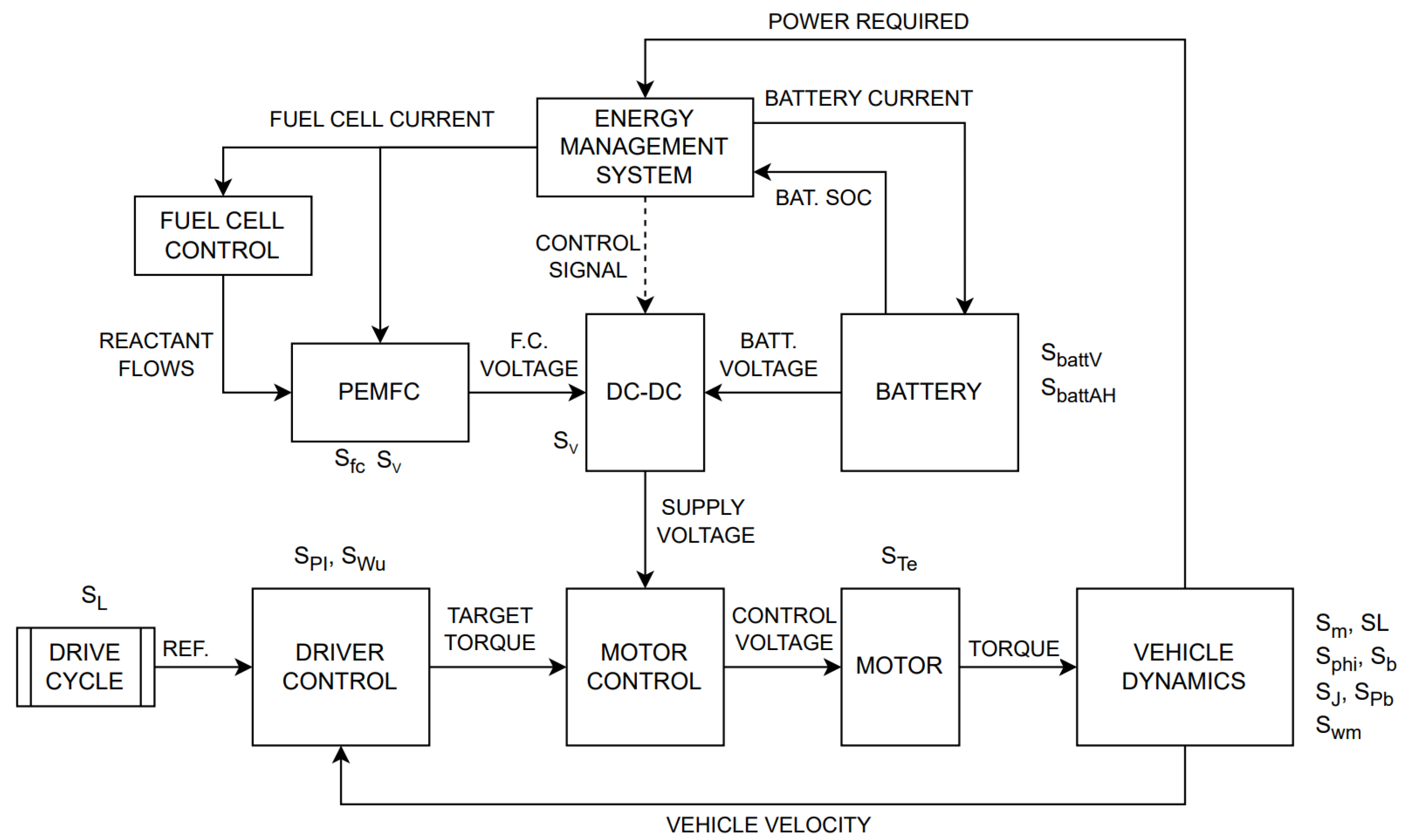
1.2. Powertrain Model

The vehicle model is comprised of vehicle, motor, fuel cell, and battery dynamics. Figure 1 shows the model architecture.

The fuel cell model is described in [1]. Individual fuel cells in the stack are modeled using the Dicks–Larminie equivalent circuit with flow model [9]. The design of the fuel cell controller is outside the scope of this paper. Relevant to the scaling methodology, the PEMFC is comprised of a stack of individual fuel cells in series with identical dynamics. The number of cells in the fuel cell stack is the only variable in the fuel cell block that will change as the system scales.

The PEMFC has a low-level ${\mathrm{H}}_{\infty }$ controller that maintains the fuel cell output voltage. Power is supplied by the fuel cell by supplying current to the vehicle; this current is considered a disturbance by the low-level controller, which subsequently manages reactant flows in order to maintain the output voltage. Figure 2 shows the control block diagram for the PEMFC. The details of this control are outside the scope of this paper.

The battery is modeled as a nonlinear RC equivalent circuit with state-of-charge (SOC) dependent parameters, as shown by Hariharan et al. [10], and shown in Figure 3. The voltage outputs of the fuel cell and battery are reconciled by a DC-DC converter before the final voltage is supplied to the motor controller.

The energy management system block represents the strategy for choosing whether to power the vehicle from the fuel cell or the battery, given the current power required by the vehicle, the battery SOC, and the capabilities of the fuel cell. The design of the energy management system is the primary area of active research. Its development, while outside the scope of this paper, is what this paper aims to support.

The driver control block uses the drive cycle reference speed and the vehicle’s actual speed to calculate target torques via proportional–integral (PI) with feedforward, Youla, ${\mathrm{H}}_{\infty }$, or hybrid Youla-H control, all of which will be discussed further.

For the results in this paper, the motor dynamics are assumed to be significantly faster than vehicle dynamics, and so the target torque is immediately applied to the vehicle dynamics if possible. The motor block may saturate the torque output, with the maximum torque available decreasing as the motor rotational speed increases. This is a nonlinear effect that the controllers compensate for by being robust. A 3-phase permanent-magnet synchronous motor (PMSM) model [1] of motor dynamics, developed via a bond graph approach in [1], allows for transient voltage estimates that are more accurate to the actual EV. The PMSM model is omitted in this paper for simplicity but may be added in the future. The PMSM model is mentioned in order to discuss the difficulties it presents in scaling its dynamics.

The vehicle dynamics account for vehicle mass, viscous friction, motor inertia, gearing, air resistance, and tire slip. Future versions of this model will also incorporate series regenerative braking to maximize energy efficiency, using friction braking only when absolutely necessary. In this paper, all braking is done with regenerative braking irrespective of battery SOC limits. Future work will incorporate these limits.

1.3. Dimensional Analysis

The Buckingham Pi (BP) theorem in dimensional analysis [11] is a common approach to developing scale system models. The BP method computes dimensionless parameters from a given set of input variables to the equation being analyzed based on the physical units of those input variables. If the dimensionless parameters are held constant when changing the parameters of the model, then the model is considered to have various potential degrees of similitude and, thus, to be representative of full-scale behavior. This method requires solving systems of linear equations and can be unwieldy when repeatedly applied. It is best suited for equations involving a large number of parameters or when an explicit relationship may not be known.

The vehicle powertrain model in question consists of many simple equations with few relevant parameters rather than fewer equations with more parameters. Rather than repeatedly applying the BP theorem, the model can be systematically scaled with an easy inspection of the governing equations with the method presented in this paper, which could be considered a simplified version of the BP theorem.

1.4. Control Methods

A proportional–integral (PI) controller with reference feedforward is examined, representing the baseline controller performance of traditional methods. The PI gains were initially determined via experimentation and then tuned by considering the closed-loop transfer functions in order to set the controller bandwidth to be the same on each controller described in this paper. In order to keep system performance constant throughout scaling magnitudes, the PI gains have a specific scaling factor to keep the dynamics constant.

Youla parameterization [12] is a technique in neoclassical control theory that provides robust controller performance, where robustness is defined as the insensitivity of system performance to changes in system parameters, such as vehicle mass, friction, etc. The Youla controller can be developed analytically, given a linear model of the plant and the desired closed-loop behavior, which in this paper is a second-order response with a damping ratio of 1.0. With an appropriately scaled model, controller tuning will be independent of the scale of the system and will not need to be performed by the user across scaling magnitudes. Due to the robust nature of Youla parameterization, performance can be maintained despite system nonlinearities that are not captured by the scaling method. Since the controller is calculated by the system parameters directly, it does not require any scaling factors specific to the controller.

${\mathrm{H}}_{\infty }$ control [12] is another neoclassical control technique that provides optimally robust performance, given the designer’s closed-loop response priorities. These priorities are represented as weighting functions on the closed-loop transfer functions, which are provided to an optimization algorithm to produce the controller transfer function that maximizes robustness given the weighting functions. Since the closed-loop sensitivity and complementary sensitivity transfer functions S and T, respectively, are ratios in the frequency domain, they do not change as the system parameters are scaled. However, the Youla transfer function Y, which represents the actuator effort, does scale with the actuator size and so must have a scaling factor applied in order for the optimization algorithm to produce the same dynamics across scaling magnitudes.

Finally, a hybrid Youla and ${\mathbf{H}}_{\infty }$ approach, referred to as the Youla-H method, is performed, which uses the poles and zeros of the Y transfer function produced by the ${\mathrm{H}}_{\infty }$ algorithm as the input to the Youla parameterization method. This allows for performance improvements without sacrificing robustness by making small adjustments to ensure that exact reference tracking is possible. This also allows for the controller to be calculated by the plant parameters without requiring a specific controller scaling factor.

All controllers are selected so that the closed-loop system bandwidth is approximately 24 rad/s. Among the other aspects, the bandwidth corresponds to the reaction speed of the controller, and keeping this metric constant makes the comparisons of tracking error, robustness, and noise attenuation between controllers meaningful when applied to a drive cycle where the reference velocity is rapidly changing. The value of 24 rad/s was found to be a good balance of tracking performance and noise attenuation, given the rate at which common drive cycles change their reference target speed.

2. Scaling Method

The scaling method utilized consists of the following steps:

1.

List equations that define the behavior of the model.

2.

Begin determining what variables and parameters will be scaled.

3.

Determine the scaling relationship for each equation.

4.

Develop the complete list of scaled variables while performing the previous step.

5.

Check for relationships that over-constrain the scaling system and decide which scaling factors are to be considered the “independent” factors input to the system.

Scaling parameters will be denoted $S_x$, where x is the parameter being scaled and are defined as shown in Equation (1).

$$S_x={\displaystyle \frac{x_{new}}{x_{original}}}={\displaystyle \frac{x_n}{x_o}}$$

(1)

Simple Example

A simple model to examine the scaling method is as follows. Suppose a mass-spring-damper system, as shown in Figure 4.

Step 1: Write the governing equation(s):

$$ma=F-kx-bv$$

(2)

Step 2: Determining the variables to be scaled: mass, length, input force, spring constant, and damping constant.

Step 3: Determine the scaling relationship for each equation. First replace each original variable with its new variable, given by $x_n=S_x{x}_o$. Since they are time derivatives of each other, the acceleration, velocity, and position can all be modified by a single length scaling parameter $S_L$. This assumes that the timescale is not being changed, otherwise the velocity and acceleration would need time-scaling factors applied.

$$S_{m}m{S}_{L}a=S_{F}F-S_{k}k{S}_{L}x-S_{b}b{S}_{L}v$$

(3)

Factoring out the length scaling results in:

$$S_{m}ma={\displaystyle \frac{S_F}{S_L}}F-S_{k}kx-S_{b}bv$$

(4)

By inspection, $S_m=S_F/S_L=S_k=S_b$ for the dynamics to remain unchanged. Satisfying this relationship only scales up or down the numerical values of the system variables as if only changing the units of the system, without changing the relationship between each variable.

The more general approach is to determine the scaling relationship required to be able to factor out all of the scalings from the equation and be left only with the variables present in the original equation. The left side $S_m$ can only be canceled out if $S_m=S_F/S_L=S_k=S_b$.

Step 4: Develop a complete list of scaled variables: $S_m,S_F,S_k,S_b$, $S_L$. This step is complete because there was only one equation. The purpose of Step 4 is to allow for the list of scalings to grow as the equations are analyzed.

Step 5: Since there was only one governing equation and that equation is easily solvable, there cannot be over-constraints. An example of a potential conflict would be the introduction of air resistance:

$$ma=F-kx-bv-{\displaystyle \frac{1}{2}}\rho v{C}_{d}A$$

(5)

which becomes:

$$S_{m}m{S}_{L}a=S_{F}F-S_{k}k{S}_{L}x-S_{b}b{S}_{L}v-{\displaystyle \frac{1}{2}}{S}_{\rho }\rho S_L^2{v}^2{S}_{Cd}{C}_d{S}_{A}A$$

(6)

This introduces a complex requirement where $S_{\rho }{S}_L{S}_{Cd}{S}_A=S_m$. The effort that goes into satisfying this requirement relative to its importance to the model determines whether air resistance or other similar aspects should be omitted from the scaling system (though not from the actual simulation model).

If air drag is omitted from the scaling system, then $ma=F-kx-bv$ is the only remaining equation defining system behavior. The resulting scaling relationship $S_m=S_F/S_L=S_k=S_b$ indicates that there are two degrees of freedom (DOFs). One independent scaling is described by $S_m=S_k=S_b$, where any one of these three can be chosen to set the other two. The second independent scaling is either the length or force scaling.

3. System Modeling

With the above example complete, the analysis of the actual EV powertrain model is described in this section. The goal of scaling this model is to preserve the velocity-tracking performance of the vehicle during drive cycles, such as the FTP75 drive cycle, and subsequently estimate the hydrogen consumption performance for different battery management strategies.

3.1. Step 1: Governing Equations

The governing equations are grouped into those relating to the vehicle, controller, and electrical dynamics.

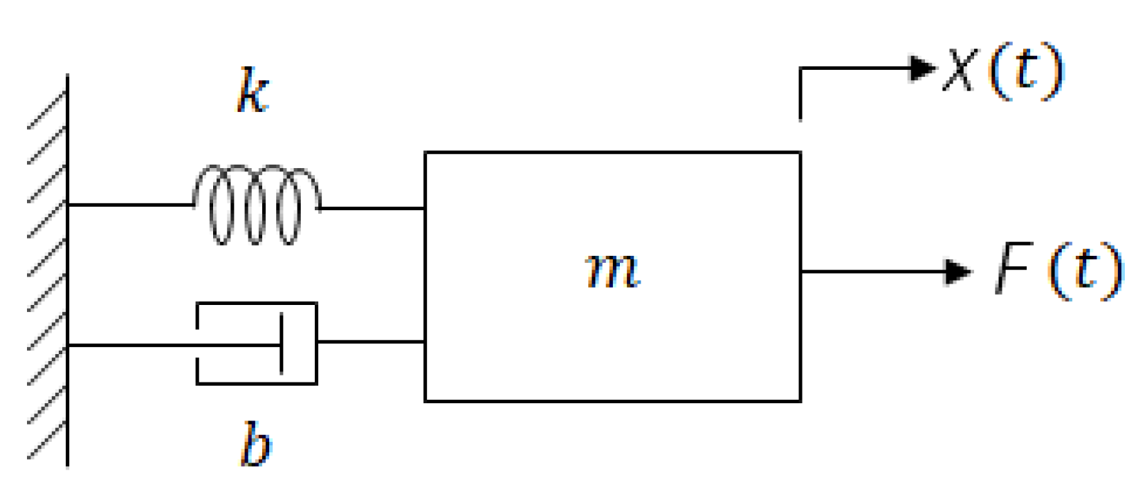
3.1.1. Vehicle Dynamics

Equation (7) represents the mechanical power imparted to the vehicle system. $F_w$ is the force at the wheel and v is the speed of the car.

$$P=F_{w}v$$

(7)

Equation (8) gives the force at the wheel, where m is the total mass of the vehicle, a is the vehicle’s acceleration, and $F_d$ is the drag force due to air resistance.

$$F_w=ma+F_d$$

(8)

Equation (9) provides the drag force, where $\rho$ is air density, v is the vehicle speed, $C_d$ is the drag coefficient, and A is the vehicle cross-sectional area.

$$F_d={\displaystyle \frac{1}{2}}\rho v{C}_{d}A$$

(9)

Equation (10) shows the relationship between the torque at the wheel and the force at the wheel, with r being the wheel radius.

$$T_w=F_{w}r$$

(10)

Equation (11) is the torque at the motor, where $\varphi$ is the gear ratio, $\eta$ is an efficiency factor in converting motor torque to wheel torque, J is the motor moment of inertia, $\alpha$ is the motor angular acceleration, b is the motor viscous friction, and ${\omega }_m$ is the motor angular velocity.

$$T_e={\displaystyle \frac{T_w}{\varphi \eta }}+J\alpha +b{\omega }_m$$

(11)

Equation (12) defines the relationship between the motor rotational velocity ${\omega }_m$ and the vehicle speed v through the gear ratio $\varphi$, where r is the wheel radius.

$${\omega }_m=\varphi {\displaystyle \frac{v}{r}}$$

(12)

Equation (13) gives the braking torque as a function of the braking friction coefficient ${\mu }_b$, the disc brake diameter $D_B$, the number of brake pads $N_B$, and the braking pressure $P_B$.

$$T_b={\mu }_b{\displaystyle \frac{\pi }{8}}{D}_B^3{N}_B{P}_B$$

(13)

3.1.2. Controller Dynamics

Equation (14) describes the output of the baseline PI plus feedforward controller that the Youla controller will be compared against. $K_p$, $K_i$, and $K_{ff}$ represent the proportional, integral, and feedforward gains, respectively. $T_{max}$ is the maximum motor torque, e is the velocity tracking error, and $v_{ref}$ is the current target velocity.

$$T_e=T_{max}(K_{p}e+K_i\int edt+K_{ff}{v}_{ref})$$

(14)

Equation (15) describes the output of ${\mathrm{H}}_{\infty }$ controller transfer function. This is required to determine the scaling factor for the actuator weighting function given to the optimization algorithm.

$$G_{CH}={\displaystyle \frac{T_e}{e}}$$

(15)

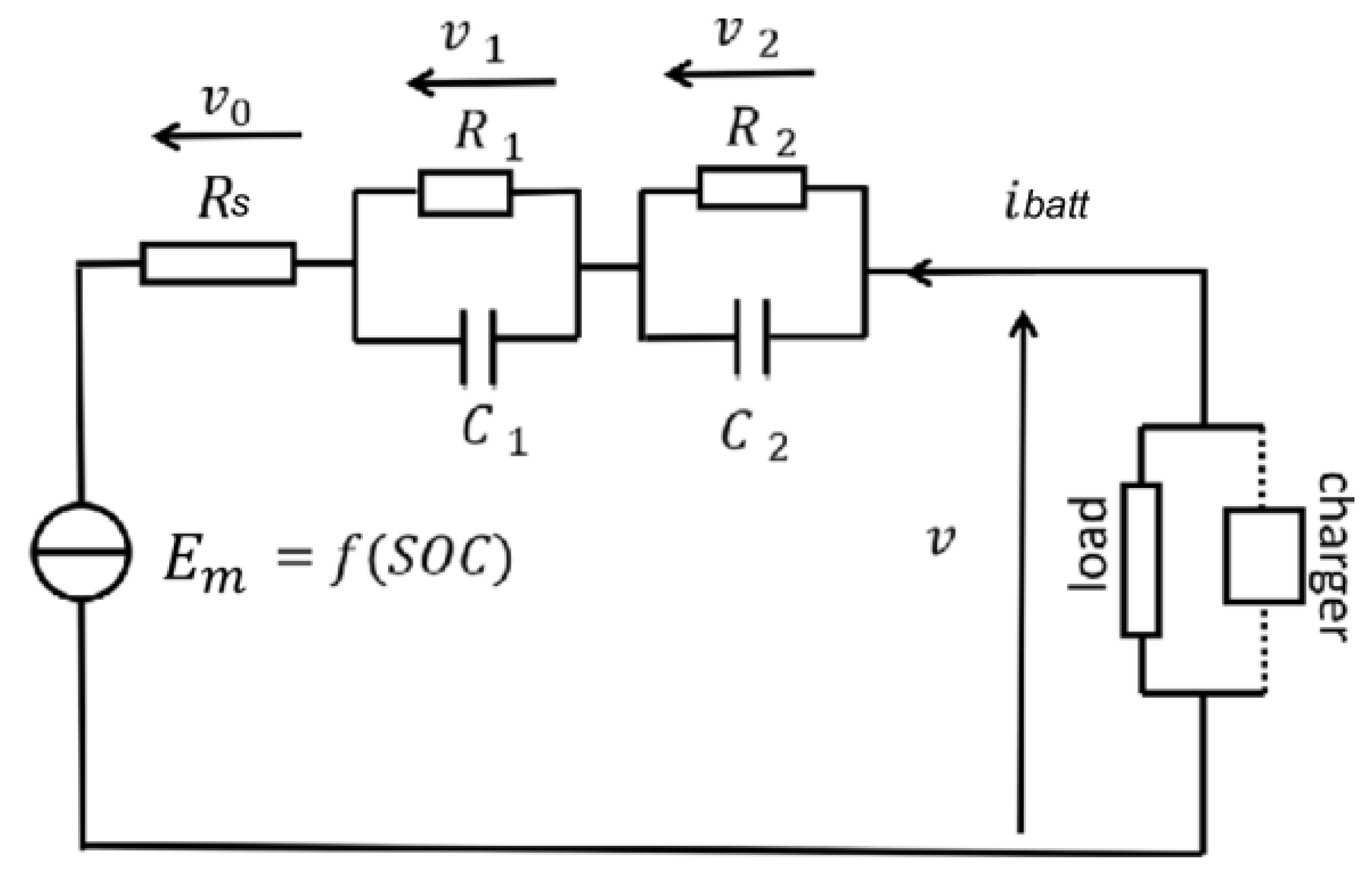
3.1.3. Electrical Dynamics

Equation (16) [1] provides the fuel cell stack voltage $V_{stack}$ in terms of the number of fuel cells N, the fuel cell internal voltage E (determined by reactant partial pressures and electrochemistry), the cell layer capacitive voltage $V_a$, and the ohmic losses $V_{ohm}$. Within the scope of this paper, the internal, capacitive, and ohmic loss voltages will be considered unchanged regardless of scaling, with the fuel cell output voltage scaling only with the number of individual fuel cells.

$$V_{stack}=N(E-V_a-V_{ohm})$$

(16)

The fundamental electrical power equation $P=IV$ can be considered when applied to the fuel cell, shown in Equation (17), where the power, current, and voltage of the fuel cell are shown.

$$P_{fc}=I_{fc}{V}_{stack}$$

(17)

The fuel cell dynamics contained in Equation (16) plus the effect of the fuel cell’s low-level controller causes voltage transients during operation. The fuel cell controller tries to hold the output voltage constant, with the fuel cell current being a disturbance to the system. The closed-loop response of the fuel cell can be abstractly approximated by a transfer function, though the real dynamics are nonlinear and cannot be described with an actual Laplace-domain transfer function. For the purposes of the scaling system, Equation (18) describes the closed-loop dynamics in response to current disturbance.

$$G_{fcVI}={\displaystyle \frac{V_{stack}\left(s\right)}{I_{fc}\left(s\right)}}$$

(18)

The battery has an empirical relationship between its output voltage and its state of charge (SOC). Since the SOC is dimensionless, the battery’s output voltage will simply scale with the overall voltage scaling, as discussed later. The battery’s capacity will scale with the energy scaling of the system.

3.2. Step 2: Determine the Scaling Variables

By inspecting Equations (7)–(16), we can develop the list of scaling variables. To simplify the analysis, the following assumptions are made:

• The vehicle velocity, acceleration, reference velocity, and tracking error all have the same length scaling factor $S_L$.
• The vehicle size parameters, such as the wheel radius, share the length scaling factor $S_L$ used for velocity.

For example, a vehicle sized down 1:10 will use a drive cycle scaled down 1:10. The initial list of scaling variables can be chosen as follows:

• $S_L$—vehicle and drive cycle length;
• $S_E$—energy/power of vehicle system;
• $S_{Fw}$—force at the wheel;
• $S_m$—vehicle mass;
• $S_{Fd}$—drag force;
• $S_{Tw}$—torque at the wheel;
• $S_{Te}$—torque at the motor;
• $S_{\varphi }$—gear ratio;
• $S_{\eta }$—motor to wheel efficiency;
• $S_J$—motor moment of inertia;
• $S_{\omega m}$—motor angular velocity;
• $S_b$—motor friction;
• $S_{Tb}$—braking torque;
• $S_{Pb}$—brake disc pressure;
• $S_{PI}$—PI controller gains;
• $S_{Wu}$—${\mathrm{H}}_{\infty }$$W_u$ weighting;
• $S_V$—system and fuel cell voltage;
• $S_{Ifc}$—fuel cell current;
• $S_{fc}$—fuel cell stack size;
• $S_{GfcVI}$—fuel cell closed-loop voltage-current ratio dynamics;
• $S_{battV}$—battery voltage;
• $S_{battAH}$—battery capacity.

This list was obtained by the following Equations (7)–(16) and writing the scaling factor for each new variable observed. A subset of these variables is shown in Figure 1 located near their respective component of the model architecture diagram and are applied to parameters in their respective blocks. By applying this scaling system, the output signals of each block are, by consequence of how the scaling parameters are defined, scaled to the appropriate degree such that the relationship between each variable in the model is invariant, with only the numerical values being evenly scaled up or down. It is important to recognize that scaling parameters are not applied to any signals between blocks; they are applied to parameters such that the output signals are scaled and shaped correctly.

3.3. Step 3: Develop Scaling Relationships

It is desirable to have the energy and length scalings be independent of each other since the size of the scale car will be determined by the existing radio-control (RC) car chassis, and so that the energy requirements of the system can be chosen separately to fit within available small-scale fuel cell power constraints.

3.3.1. Vehicle Scaling

Starting with Equation (7), the mechanical power imparted to the system, we can determine the scaling relationship by first rewriting Equation (7) and replacing each original variable with their respective new variable, given by $x_n=S_x{x}_o$, as shown in Equation (19).

$$S_{E}P=S_{Fw}{F}_w{S}_{L}v$$

(19)

Equation (19) represents Equation (7) for the “new” version of each variable, with those new variables replaced with $S_x{x}_o$. Since $S_x=x_n/x_o$, dividing the left and right sides of Equation (19) by the left and right sides of Equation (7) results in Equation (20) below, which is the constitutive scaling relationship for Equation (7).

$$S_E=S_{Fw}{S}_L\to S_E=S_m{S}_L^2$$

(20)

The energy scaling of the system (for example, scaling from 40 kW peak power down to 4 W) has to be equal to the scaling of the force at the wheel times the overall length scaling. As shown subsequently in Equation (8), this can be further simplified to the mass scaling times the length scaling squared. On its own, this relationship allows for two of three between energy, mass, and length to be independent degrees of freedom with the third being constrained. For considering the degrees of freedom, the mass scaling $S_m$ can be considered an alternative representation of the energy scaling’s degree of freedom.

For subsequent equations in this section, an abridged version of the process followed above is used. Only the final scaling relationship is described, as determined via analysis and inspection. Each relationship will also be reduced to the core independent scalings $S_L$ and, interchangeably, $S_E$ or $S_m$.

The scaling relationship for Equation (8), the calculation of the force at the wheel, is given by Equation (21).

$$S_{Fw}=S_m{S}_L=S_{Fd}$$

(21)

The scaling relationship for Equation (9), the drag force, is given by Equation (22). This assumes the air density and drag coefficient remain unchanged and that the velocity and frontal area scalings share the same core length scaling.

$$S_{Fd}=S_L^3\to S_m=S_L^2$$

(22)

Note that this presents a constraint to the relationship between length and mass/energy scaling, which is undesirable. This will be discussed in more detail in Step 5 of the process.

In the scaling relationship for Equation (10), the calculation of the torque at the wheel is given by Equation (23).

$$S_{Tw}=S_{Fw}{S}_L\to S_{Tw}=S_E$$

(23)

In the scaling relationship for Equation (11), the calculation of the torque at the motor is given by Equation (24).

$$S_{Te}={\displaystyle \frac{S_{Tw}}{S_{\varphi }{S}_{\eta }}}=S_J{S}_{\omega m}=S_b{S}_{\omega m}$$

(24)

Equation (24) introduces two new degrees of freedom, observable by the fact that Equation (23) gives $S_{Tw}=S_E$, which does not constrain the motor inertia, motor friction, gear ratio, or conversion efficiency scalings. The gear ratio and efficiency scalings $S_{\varphi }$ and $S_{\eta }$ are selected as the independent scalings, since the drivetrain gear ratio may change between the full-scale and scaled-down vehicles and since the conversion efficiency is an empirical adjustment factor to compensate for unmodeled losses.

In the scaling relationship for Equation (12), the motor angular velocity is given by Equation (25). Since the vehicle velocity and tire radius both scale by $S_L$, this simplifies to the motor speed scaling being equal to the gear ratio scaling. When the drive cycle and vehicle dimensional scales are the same, the angular velocity at the wheel (rather than the motor) is held constant.

$$S_{\omega m}=S_{\varphi }{\displaystyle \frac{S_L}{S_L}}\to S_{\omega m}=S_{\varphi }$$

(25)

Considering Equation (25) and the additional gear ratio and efficiency independent scalings, an equivalent form of Equation (24) is given below in Equation (26).

$$S_J=S_b={\displaystyle \frac{S_E}{S_{\varphi }^2{S}_{\eta }}}$$

(26)

The scaling relationship for Equation (13), the friction braking torque, is given by Equation (27). This assumes that the coefficient of friction and the number of brake pads stays constant and that the size of the disc brake scales with the overall length scaling. To relate the braking torque to the rest of the vehicle, the braking torque must additionally scale with the torque at the wheel.

$$S_{Tb}=S_L^3{S}_{Pb}=S_{Tw}\to S_{Pb}=S_m/S_L$$

(27)

3.3.2. Controller Scaling

In the scaling relationship for Equation (14), the PI controller gains is given by Equation (28). Note that in Equation (14), the left and right sides of the equation are both multiplied by a motor torque, so the scalings for the terms inside the parentheses are equal to a scaling of 1 due to the motor torque scaling factors canceling on both sides. Also note that the error, its time integral, and the reference velocity all share the same overall length scaling.

$$S_{PI}={\displaystyle \frac{1}{S_L}}$$

(28)

The Youla controller does not require a specific scaling factor since its controller is determined by the plant model parameters directly.

The ${\mathrm{H}}_{\infty }$ controller is not directly scaled by any factor. Instead, the weighting function $W_u$ that penalizes actuator effort must be scaled to account for the change in the actuator effort relative to input commands as the vehicle parameters are scaled so that the ${\mathrm{H}}_{\infty }$ optimization produces the same controller poles and zeros.

$$S_{Wu}={\displaystyle \frac{S_L}{S_{Te}}}\to S_{Wu}={\displaystyle \frac{S_L{S}_{\varphi }{S}_{\eta }}{S_E}}$$

(29)

3.3.3. Electrical Scaling

In the scaling relationship for Equation (16), the fuel cell stack voltage is given by Equation (30). The terms other than the number of fuel cells in the fuel cell stack are approximated as being constant throughout system scalings.

$$S_V=S_{fc}$$

(30)

Since $S_V$ has not appeared elsewhere, it can be considered a new independent scaling.

In the scaling relationship for Equation (17), the electrical power relationship for the fuel cell is shown in Equation (31).

$$S_E=S_{Ifc}{S}_V\to S_{Ifc}={\displaystyle \frac{S_E}{S_V}}$$

(31)

For Equation (18), the scaling relationship is shown below. Note that since $G_{fcVI}$ is already a ratio, its scaling needs to be equal to 1 if the transient voltage dynamics are to be held constant. This relationship thus creates a constraint between the energy and voltage scalings, which is undesirable.

$$S_{GfcVI}={\displaystyle \frac{S_V}{S_{Ifc}}}\to S_{GfcVI}={\displaystyle \frac{S_V^2}{S_E}}$$

(32)

For the battery, Equations (33) and (34) describe the relationships for the battery voltage and capacity.

$$S_{battV}=S_V$$

(33)

$$S_{battAH}=S_E$$

(34)

3.4. Step 4: Complete List

Auxiliary scalings can be determined in this step if necessary. Because this scaling system was completed prior to the writing of this paper, it is not necessary in this case.

3.5. Step 5: Resolve Constraints and Choose Independent Scalings

Similar to the Simple Example, the drag force equation introduces an overconstraint to the system, even with its simplifications. Equation (22) shows $S_{Fd}=S_L^3$. Combined with Equation (21), this simplifies to $S_m=S_L^2$. This is solvable, but in the context of this simulation model, it is desirable to control the mass (or energy) and the overall length independently, so the scaling relationship defined by Equation (22) will be omitted from the scaling system. Thus, the relative effect of air drag will not exactly scale with the rest of the system. In our case, this is an acceptable approximation, since the modeled air drag will still be scaled down with the frontal area and velocity, and so the change in dynamics is small for reasonable scaling magnitudes.

The second overconstrained relationship is in Equation (32). Since energy and voltage requirements are set by implementation constraints in constructing the actual scale vehicle, the energy and voltage scalings must be independent of each other. Omitting Equation (32) resolves this issue, at the cost of the transient voltage dynamics changing in relative size. This is acceptable as long as the scaling of the hydrogen consumption of the system is still effectively described by the energy scaling, and as long as the voltage transients do not present implementation issues on either the full-scale or scaled vehicles.

By analyzing Equations (20)–(27), the vehicle scalings, it can be observed that there are four degrees of freedom. The controller scalings are entirely dependent on the vehicle scaling factors and so do not introduce any additional DOFs. The electrical scalings introduce only one extra degree of freedom, being the system voltage. Therefore, the selected independent scaling factors are as follows:

• $S_L$—vehicle and drive cycle length;
• $S_E$—energy/power of vehicle system;
• $S_{\varphi }$—gear ratio;
• $S_{\eta }$—motor to wheel efficiency;
• $S_V$—voltage.

The efficiency scaling only affects the motor–wheel efficiency relationship. The length, energy, and gear ratio scalings define every other vehicle and controller scaling not in the above list, such as the mass scaling. To implement in code, Equations (20)–(34) are simply listed prior to running the simulation model, ordered in such a way that the independent scaling factors are defined first and all others are defined in whatever order is most convenient. For example, Equation (20) can be rewritten as $S_{Fw}=S_E/S_L$, and subsequently Equation (21) as $S_m=S_{Fw}/S_L$ or $S_m=S_E/S_L^2$.

Note that the mass could have been selected as the independent variable instead of energy. In the context of this paper, energy is chosen so that the hydrogen consumption can be conveniently selected, which is more important for this model than directly defining the mass. However, the two scenarios are mathematically equivalent.

3.6. Nonlinearities and Simulation Difficulties

This scaling system works very well across a wide range of scaling magnitudes. However, there are some nonlinearities that do not perfectly scale system dynamics. The air resistance mentioned before is one aspect, as well as the voltage, reactant flow, and partial pressure dynamics of individual fuel cells. The fuel cell controller is a robust controller and so is able to compensate for the changes in relative dynamics as the system is scaled. The battery voltage–capacity relationship is also not linear, so the SOC of the battery does not stay exactly the same across scalings.

The PMSM motor model was originally part of the scaling system, with the motor resistances, inductances, and low-level controller gains being scaled along with the model. However, this model was too nonlinear to stably scale to very small values. This results in the loss of transient voltage estimates in the model. Future work may reincorporate the PMSM model by utilizing a linearized version of its dynamics to perform better estimations of voltage transients.

The development of the scaling system required trial and error to discover every required scaling factor. The series regenerative braking system initially was difficult to scale, as the regenerative braking scaled with the motor torque and was affected by the gear ratio, but friction braking was a separate system that bypassed the gear ratio. The input to the regenerative braking system was a single target braking torque at the motor, and so the friction braking system required particular attention to keep its effects on the vehicle dynamics constant.

This model is a stiff system and can run into solver difficulties if a non-optimal solver algorithm is selected. A modified Rosenbrock solver is utilized for the results in this paper, which was found to handle the model stiffness and high degrees of scaling magnitudes well.

4. Controller Design

In this section, the PI, Youla, ${\mathrm{H}}_{\infty }$, and combined Youla plus ${\mathrm{H}}_{\infty }$ (Youla-H) methods are developed utilizing both open-loop and closed-loop analyses. The standard transfer functions [12] used throughout are defined below.

• $G_P$—plant transfer function.
• $G_C$—controller transfer function.
• $L=G_C{G}_P$—open-loop transfer function/return ratio, represents open-loop system response to reference input.
• $T=L/(1+L)$—complementary sensitivity transfer function, relates to closed-loop reference tracking relative to reference input.
• $S=1/(1+L)$—sensitivity transfer function, relates to closed-loop disturbance and plant parameter variation sensitivity.
• $Y=G_C/(1+L)$—Youla transfer function, relates to closed-loop actuator effort relative to reference input.

In loop shaping, there are ideal shapes for each of these transfer functions. These characteristics are the following:

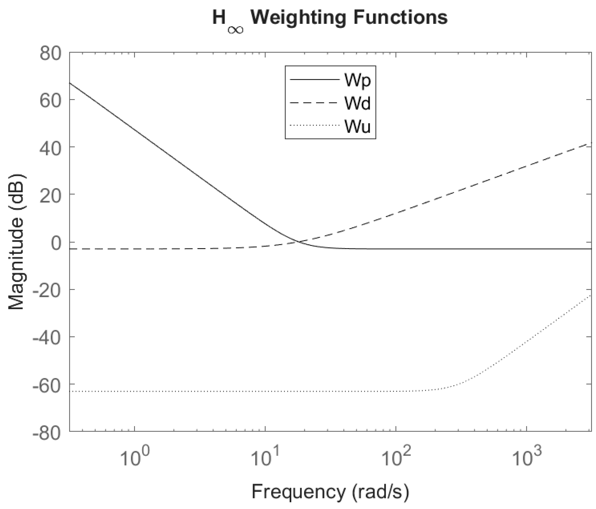
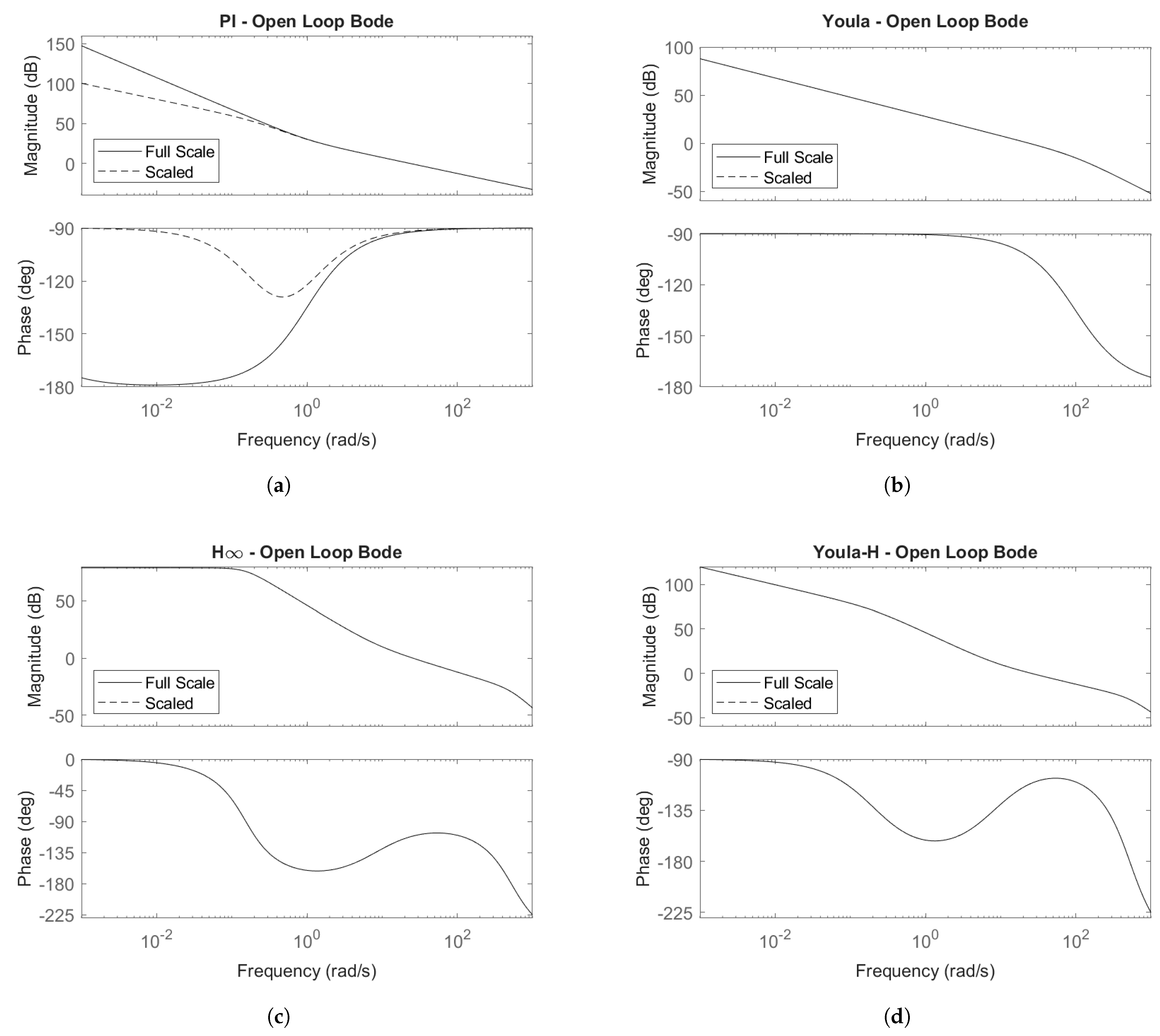
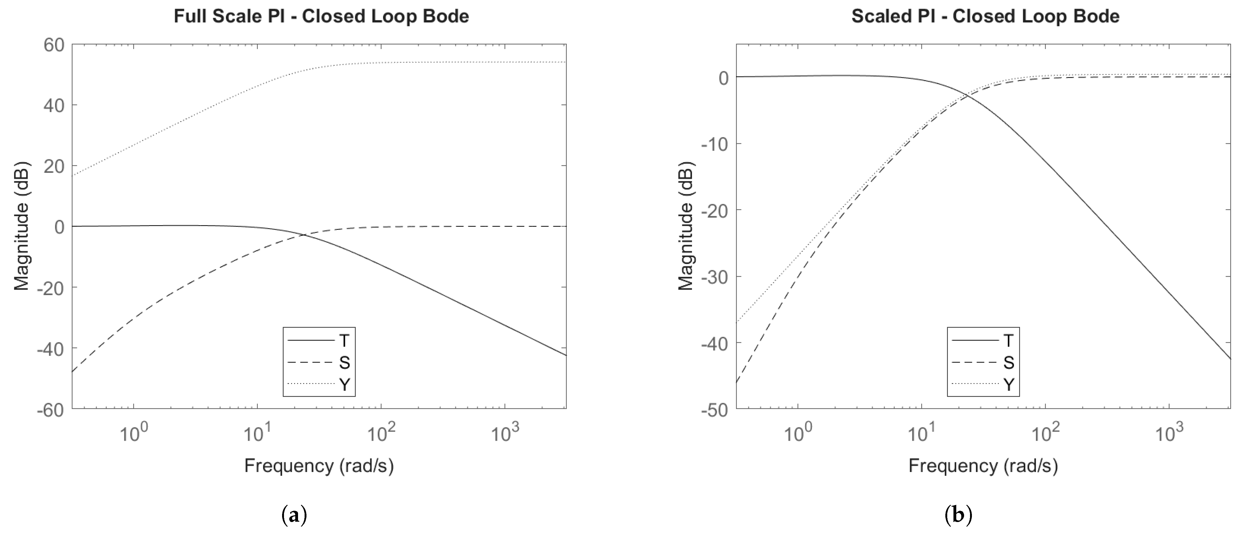
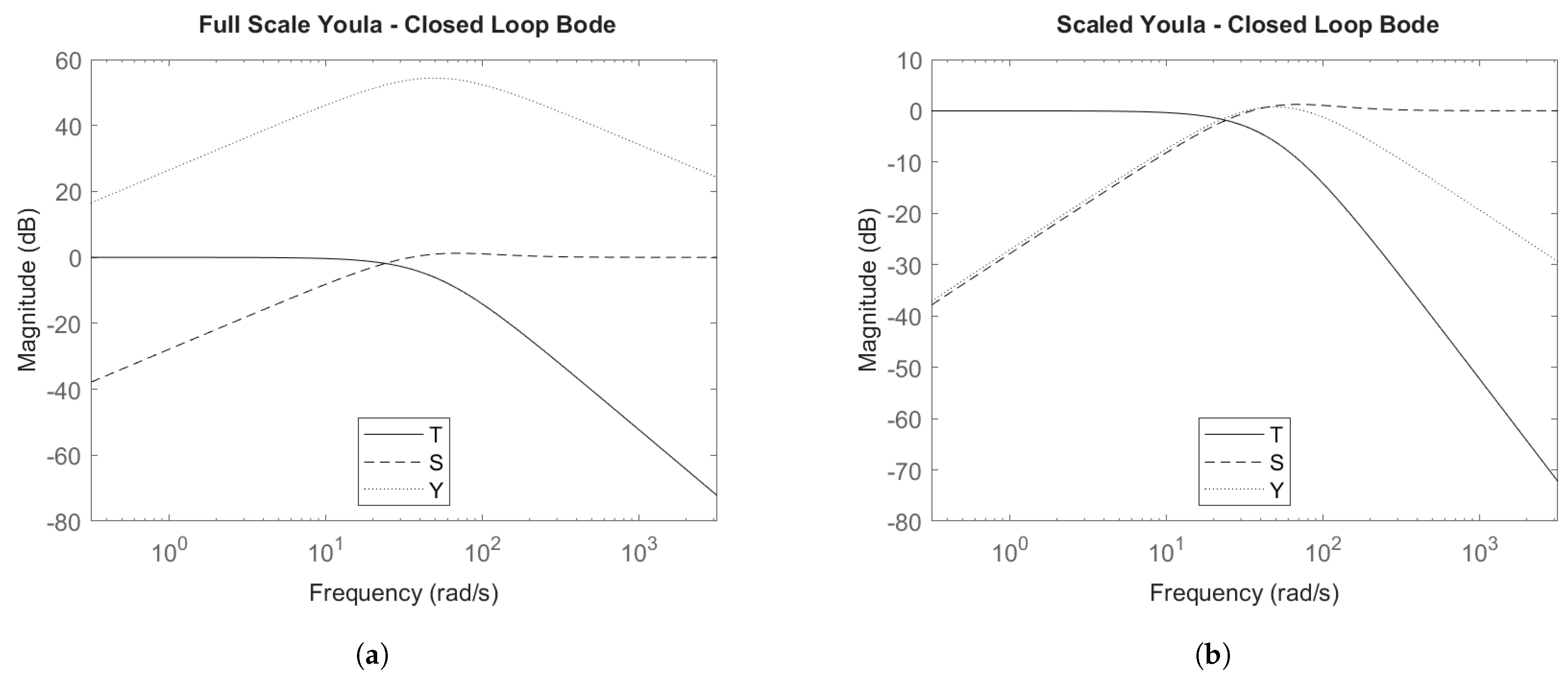
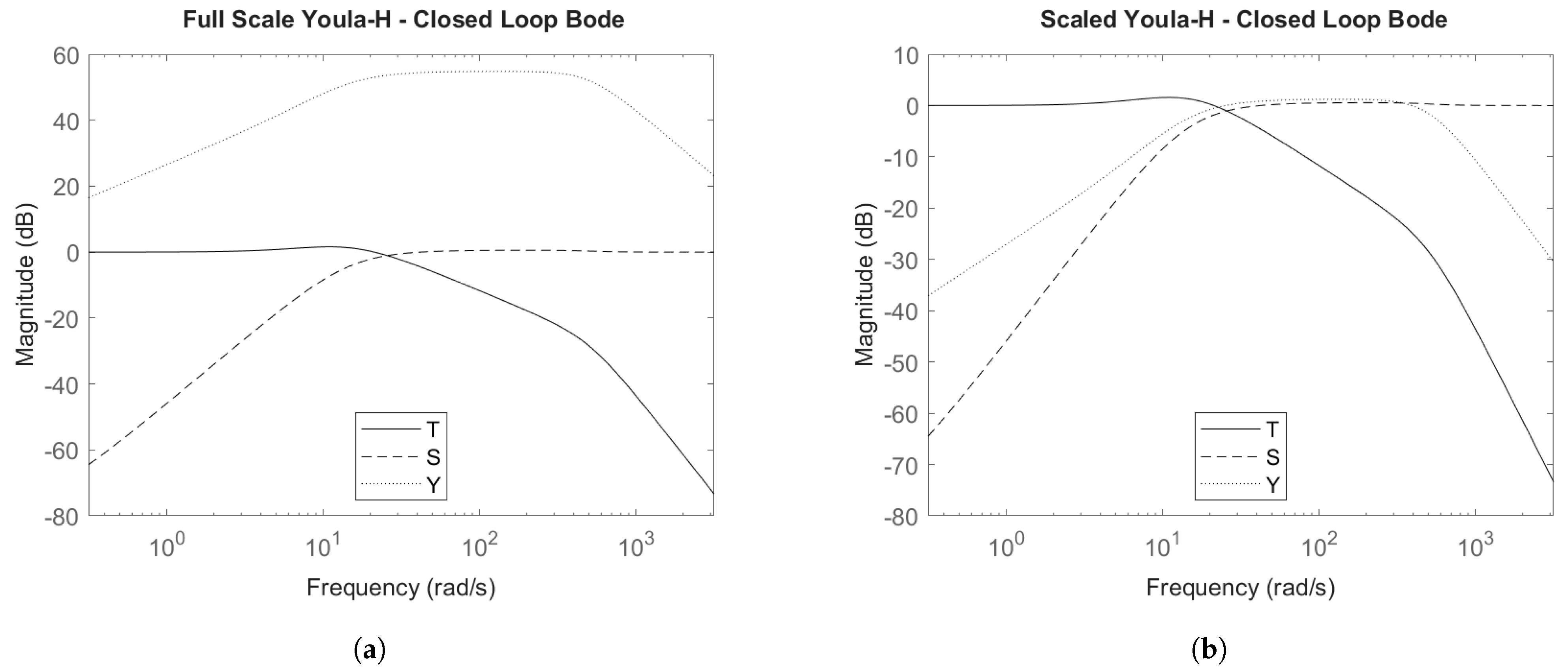
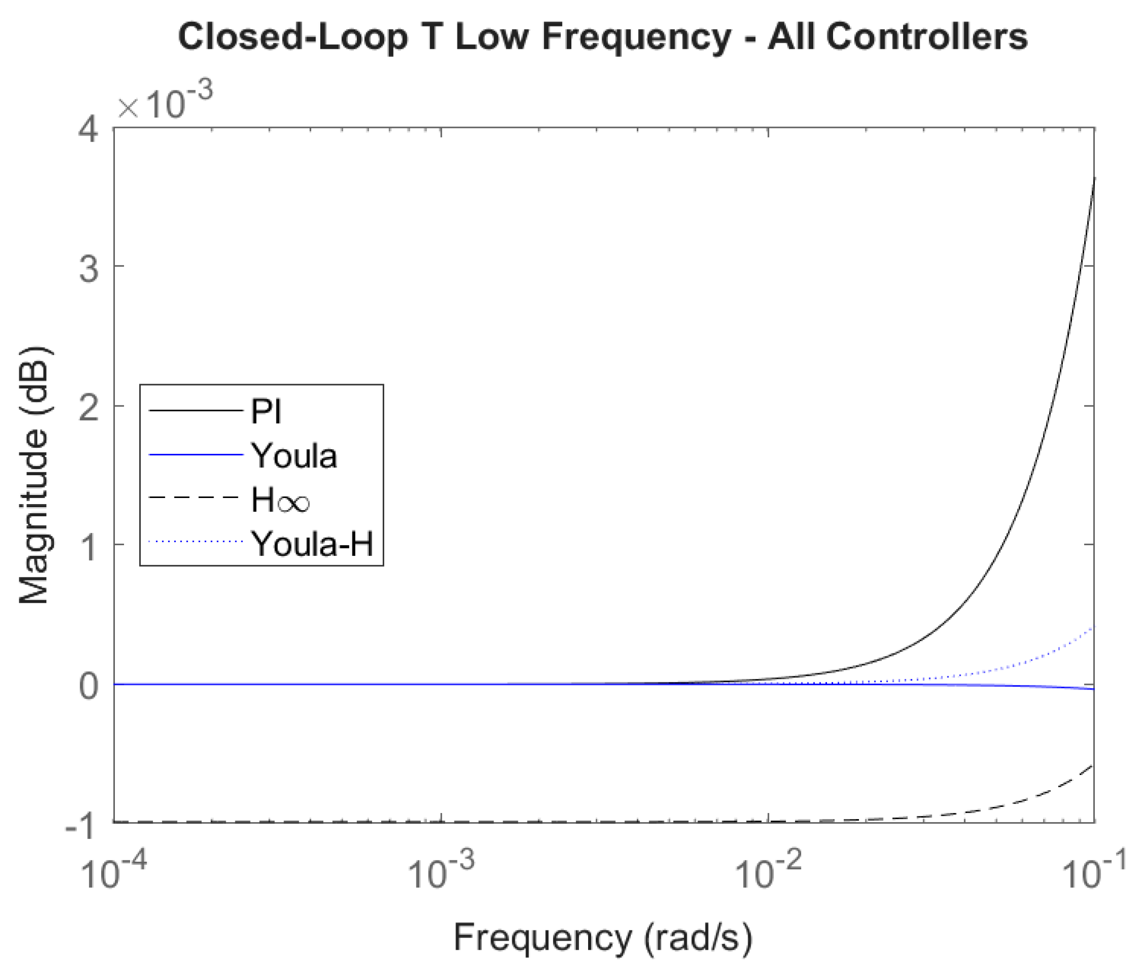
• T is exactly 0 dB in low frequencies to track reference signals and low in high frequencies to attenuate sensor noise.
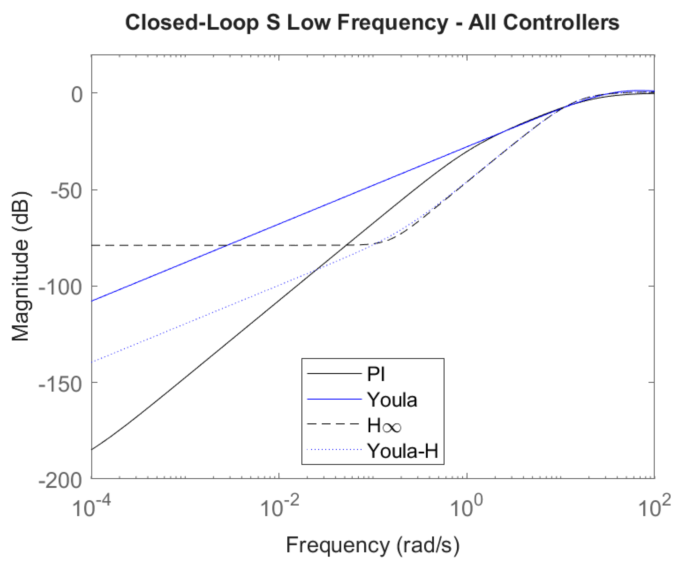
• S is low in low frequencies to attenuate disturbance and parameter variation effects.
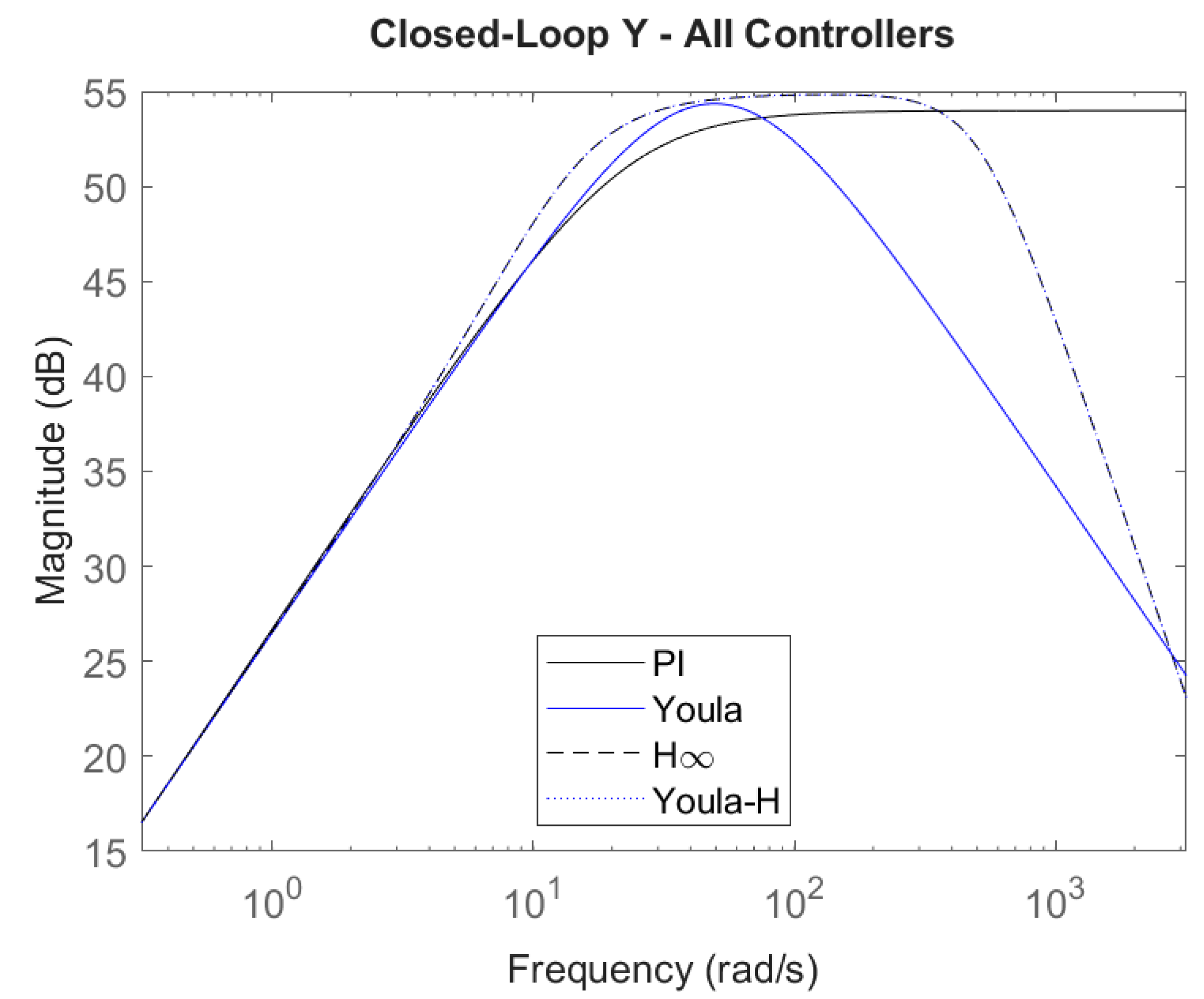
• Y is low in high frequencies to attenuate sensor noise, limiting actuator jitter.
• The maximum magnitude of S is as close to 0 dB as possible, as this relates to system robustness.
• The maximum magnitude of Y is as low as feasible, as this determines the required actuator size.

4.1. Linear Plant Model

A simplified linear model of the vehicle is required to develop the closed-loop transfer functions of each controller and is shown in Figure 5.

This model omits air drag, tire slip, friction braking, and motor electrical dynamics. The plant transfer function $G_P$ equivalent to the block diagram in Figure 5 is shown in Equation (35).

$$G_P={\displaystyle \frac{v}{T_e}}={\displaystyle \frac{\frac{\varphi }{mr}}{s+\frac{b{\varphi }^2}{m{r}^2}}}$$

(35)

where m is given in Equation (36), r is the tire radius, b is the motor friction coefficient, and $\varphi$ is the gear ratio.

$$m=m_v+{\displaystyle \frac{{\varphi }^2}{r^2}}J$$

(36)

The total effective mass m is a function of the vehicle mass $m_v$, $\varphi$, r, and the motor’s moment of inertia J.

$G_P$ is a stable first-order transfer function, making it an easy system to control with a variety of control methods. However, this is the approximate linear representation used only for control design. All simulations are performed on the nonlinear plant and actuator model.

4.2. PI Control

For the PI output torque defined in Equation (14), the controller transfer function $G_{CPI}=T_e/e$ can be described in Equation (37).

$$G_{CPI}=T_{max}(K_p+{\displaystyle \frac{1}{s}}{K}_i+K_{ff}{\displaystyle \frac{v_{ref}}{e}})$$

(37)

However, $v_{ref}$ and e must be factored out. Given that $v_{ref}/e=1-v/e=1-G_C{G}_P$, Equation (38) provides the equivalent $G_C$ for the PI controller.

$$G_{CPI}=T_{max}{\displaystyle \frac{(K_p+K_{ff})s+K_i}{s(1+K_{ff}{G}_P)}}$$

(38)

This $G_{CPI}$ can be used in conjunction with the linear plant $G_P$ to calculate the T, S, and Y transfer functions and, subsequently, the crossover frequency. The full-scale gains of $K_p=1.0$, $K_i=1.0$, and $K_{ff}=0.001$ were experimentally determined to set the crossover frequency close to 24 rad/s, setting the bandwidth to be the same as the other controllers.

4.3. Youla Control

The driver controller was originally implemented as a proportional–integral controller with reference feed-forward. To improve on the robustness and in order to keep the closed-loop system behavior constant throughout scalings, a controller is developed in this section using Youla parameterization.

The form of the Youla transfer function is chosen to cancel the stable plant pole and implement a second-order response, as shown in Equation (39).

$$Y={\displaystyle \frac{K\left(\frac{m{r}^2}{b{\varphi }^2}s+1\right)}{s^2+2\zeta {\omega }_{n}s+{{\omega }_n}^2}}$$

(39)

Additional parameters are the Youla gain K, the second-order natural frequency ${\omega }_n$, and the second-order damping ratio $\zeta$. The gain K will be determined analytically in Equation (41) to ensure exact reference tracking, while the natural frequency ${\omega }_n$ will be set as a function of the desired bandwidth crossover frequency ${\omega }_c$ and damping ratio. The chosen form of Youla has a zero to cancel the plant stable pole of $G_P$ in addition to the desired second-order pole, which will become the system’s reference tracking response behavior.

Second-order dynamics are the desired closed-loop behavior so that the Y transfer function is strictly proper. This ensures that Y rolls off and has a very low magnitude in high frequencies, ensuring good noise attenuation on the actuator.

The closed-loop complementary sensitivity transfer function is given by $T=Y{G}_P$, as shown in Equation (40).

$$T={\displaystyle \frac{Kr}{b\varphi \left(s^2+2\zeta {\omega }_{n}s+{{\omega }_n}^2\right)}}$$

(40)

To ensure reference tracking at low frequencies, $T\left(s\right)$ at $s=0$ must equal 1. Solving $T\left(0\right)$ for K results in Equation (41).

$$K={\displaystyle \frac{b\varphi }{r}}{\omega }_n^2$$

(41)

Inserting Equation (41) into Equation (40) results in Equation (42), describing the simple linear system’s closed-loop behavior from reference input r to the vehicle speed v for a step input.

$$T={\displaystyle \frac{{\omega }_n^2}{s^2+2\zeta {\omega }_{n}s+{\omega }_n^2}}$$

(42)

The closed-loop sensitivity transfer function is given by $S=1-T$, which is analytically shown in Equation (43).

$$S={\displaystyle \frac{s(s+2\zeta {\omega }_n)}{s^2+2\zeta {\omega }_{n}s+{\omega }_n^2}}$$

(43)

Inserting Equation (41) into Equation (39) results in Equation (44), describing the linearized system’s closed-loop behavior from reference input r to the controller’s command effort $T_e$ for a step input.

$$Y={\displaystyle \frac{{\omega }_n^2\frac{b\varphi }{r}(\frac{m{r}^2}{b{\varphi }^2}s+1)}{s^2+2\zeta {\omega }_{n}s+{\omega }_n^2}}$$

(44)

Finally, the controller transfer function is given by $G_{CY}=Y/S$, as shown in Equation (45).

$$G_{CY}={\displaystyle \frac{{\omega }_n^2\frac{b\varphi }{r}(\frac{m{r}^2}{b{\varphi }^2}s+1)}{s(s+\sqrt{2}{\omega }_n)}}$$

(45)

In order to set the closed-loop system bandwidth to the desired crossover frequency ${\omega }_c=24$ rad/s, the open-loop transfer function L must have a magnitude of 1 at ${\omega }_c$. L is given in Equation (46) and its magnitude for $s=j{\omega }_c$ in Equation (47).

$$L={\displaystyle \frac{{\omega }_n^2}{s(s+2\zeta {\omega }_n)}}$$

(46)

$$|L\left(j{\omega }_c\right)|={\displaystyle \frac{{\omega }_n^2}{{\omega }_c\sqrt{{\omega }_c^2+4{\omega }_n^2{\zeta }^2}}}$$

(47)

Solving for ${\omega }_n$ when $\left|L\right|=1$ results in Equation (48).

$${\omega }_n={\omega }_c\sqrt{2{\zeta }^2+\sqrt{4{\zeta }^4+1}}$$

(48)

Note that it is not necessary to analytically determine the parameters to set the bandwidth to a particular value. Setting the bandwidth could be completed iteratively by inspecting the Bode magnitude plots of T and S. The analytical solution is demonstrated to provide another option to the designer.

4.4. $H_{\infty }$ Control

The ${\mathrm{H}}_{\infty }$ algorithm requires the linear plant $G_P$ and weighting functions to calculate an optimal controller. The weighting functions can be chosen to describe closed-loop behavior that matches the desirable loop shapes described in the Controller Design section. The cost function weights are $W_p$ applied to S, $W_d$ applied to T, and $W_u$ applied to Y. The optimally robust controller will be the one that minimizes the maximum magnitude of any entry in the vector ${[W_{p}S,W_{d}T,W_{u}Y]}^T$.

The weighting functions require low-frequency and high-frequency gains and a break frequency as inputs. To meet the bandwidth of 24 rad/s, a break frequency for $W_p$ and $W_d$ of 18 rad/s was chosen iteratively in order to make the final T and S functions cross over around 24 rad/s. A break frequency of 300 rad/s was chosen for $W_u$, as it partially defines the frequencies past which the actuator should attenuate sensor noise. Further, the order of the weight functions must be selected, which describes the rate at which the weighting functions rise between their low- and high-frequency gains. The $W_d$ weight has an order of 1, as the T transfer function does not need to roll off particularly quickly. The $W_p$ and $W_u$ weights have an order of 2 in order to force the S transfer function to have a lower gain in low frequencies to better attenuate parameter variations and to force the Y transfer function to lower its gain faster to better attenuate sensor noise. Figure 6 shows these weighting functions for the full-scale model.

Note that $W_p$ and $W_d$ do not change as the system scales, while $W_u$ is multiplied by $S_{Wu}$ to counter the shift in Y as the actuator becomes larger or smaller relative to the reference signal.

The controller output by the ${\mathrm{H}}_{\infty }$ optimization is given in Equation (49) for the full-scale model. Note that scaled versions of this controller will only differ in the static gain value. The pole and zero locations will stay the same across scalings.

$$G_{CH}={\displaystyle \frac{2189.9(s+8.225)(s+4.316\times {10}^{-5})(s^2+5.045\times {10}^{4}s+1.273\times {10}^9)}{(s+1.926\times {10}^4)(s^2+0.2141s+0.02291)(s^2+747.5s+2.795\times {10}^5)}}$$

(49)

This is a high-order controller, which is a natural result of finely optimizing the system and the weighting functions. Using $G_{CH}$ and $G_P$, the T, S, and Y transfer functions can be calculated. For brevity, they will not be written out but can be graphically seen in the relevant Bode plots in the Bode Plot Comparisons section.

However, an important characteristic of the T transfer function that corresponds to this plant and controller is that $T\left(0\right)=0.99989$, which is very slightly below 1.0. Note that $T\left(0\right)$ represents the ratio of the system output to the target reference value for a step input, thus being slightly below 1.0 indicates that the controller may undershoot its reference value. The weights could be tweaked in order to force $T\left(0\right)=1.0$, but a faster way to improve performance without sacrificing robustness would be the hybrid Youla and ${\mathrm{H}}_{\infty }$ method described in the next section.

4.5. Hybrid Youla-H Control

The hybrid “Youla-H” method takes the Y transfer function from the ${\mathrm{H}}_{\infty }$ optimization and applies it to the Youla control design method shown in the Youla Control section. The goal is to perform further tuning to the ${\mathrm{H}}_{\infty }$ output for even better performance and/or robustness. Since the T transfer function for $G_{CH}$ is slightly below 1.0, a very slight change to the static gain of Y while keeping the poles and zeros the same will create a new controller that can exactly track low-frequency reference inputs.

By replacing the static gain of Y from the ${\mathrm{H}}_{\infty }$ controller with the variable K, we get the Youla-H Y shown in Equation (50).

$$Y={\displaystyle \frac{K(s+8.225)(s+4.316\times {10}^{-5})(s^2+5.045\times {10}^{4}s+1.273\times {10}^9)}{(s+1.926\times {10}^4)(s^2+25.89s+216)(s^2+721.8s+2.607\times {10}^5)}}$$

(50)

Using $T=Y{G}_P$ and setting $T\left(0\right)=1$, this allows for the Y gain K to be calculated to achieve precise reference tracking. The value of K will depend on the plant parameters in $G_P$. The resulting controller is described in Equation (51).

$$G_{CYH}={\displaystyle \frac{K(s+8.225)(s+4.316\times {10}^{-5})(s^2+5.045\times {10}^{4}s+1.273\times {10}^9)}{s(s+1.926\times {10}^4)(s+0.2113)(s^2+747.5s+2.795\times {10}^5)}}$$

(51)

One particular distinction between $G_{CYH}$ and $G_{CH}$ is that the Youla-H controller has a pure integrator, caused by requiring exact step reference tracking.

4.6. Controller Transfer Function Comparisons

Controller characteristics can be compared and evaluated prior to considering simulation output data. Note that the comparisons in this section necessarily use the linear plant $G_P$ as the evaluation basis, whereas simulation results use the nonlinear plant. The effect of nonlinearities can be estimated with the linear plant analysis by considering system robustness.

4.6.1. Open-Loop Bode Plots

Using the linearized plant model $G_P$, Bode plots of the loop transfer function L can be plotted in order to explore gain and phase margins. Note that L represents the response of the plant and controller if there is no feedback and is the response of the open-loop system to a reference input.

In Figure 7, the open-loop Bode plots are shown for the PI, Youla, ${\mathrm{H}}_{\infty }$, and Youla-H controllers.

The PI and Youla controllers have an infinite gain margin, while the ${\mathrm{H}}_{\infty }$ and Youla-H controllers have a gain margin of 29.4 dB. The phase margins for the PI, Youla, ${\mathrm{H}}_{\infty }$, and Youla-H controllers are, respectively, 88°, 76°, 69°, and 69°.

The open-loop Bode plots are identical between the full-scale and scaled scenarios for the Youla, ${\mathrm{H}}_{\infty }$, and Youla-H controllers, indicating that the scaling system for both the plant and controllers is correct. Refer to

Table 1. System and control parameters.

Parameters	Scaling	Full Scale Value	Scaled Value	Notes
Energy	1:50,000	-	-	Independent scaling
Length	1:10	-	-	Independent scaling
Gear Ratio	1:10.453	10.453	1	Independent scaling
Efficiency	1:1	95%	95%	Independent scaling
Voltage [V]	8:720	720	8	Independent scaling
Mass [kg]	1:500	2242	4.48	Vehicle mass
Force at Wheel [N]	1:5000	-	-
Torque at Wheel [Nm]	1:50,000	-	-
Torque at Motor [Nm]	1:4784	500	0.105	Maximum value
Motor Speed [rpm]	1:10.453	21,000	2009	Maximum value
Motor Inertia [kg$m^2$]	1:458	3.50 × ${10}^{-2}$	7.65 × ${10}^{-5}$
Motor Friction [Nm s/rad]	1:458	1.10 × ${10}^{-4}$	2.40 × ${10}^{-7}$
Braking Pressure [kPa]	1:50	5000	100	Friction braking only
Proportional Gain [1/kph]	10:1	1.0	10	Outputs normalized torque
Integral Gain [1/kph]	10:1	1.0	10	Outputs normalized torque
Feedforward Gain [1/kph]	10:1	0.001	0.01	Outputs normalized torque
${\mathrm{H}}_{\infty }$ $W_u$ Weighting [m/Nm]	478:1	0.001	0.478	Cost function weight

for the scaling values used in the “Scaled” scenario. For the PI controller, there is a difference in its L transfer function between full-scale and scaled-down models due to the effect of reference feedforward. If feedforward were removed ($K_{ff}=0$), there would not be a difference between full-scale and scaled L Bode plots for the PI controller. The feedforward shifts one of the poles further from the imaginary axis. This could potentially be fixed by scaling the feedforward gain differently than the other controller gains, but this is unnecessary due to the closed-loop response not changing between full-scale and scaled-down scenarios, as shown in the next section.

4.6.2. Closed-Loop Bode Plots

To recap the Controller Design section, the T function describes the ratio of the closed-loop system’s output to an input reference and to sensor noise at the plotted frequencies, among other characteristics. The S plot describes how sensitive the system response is to variations in plant parameters and to unmodeled system dynamics at the given frequencies. The Y plot shows the effort by the actuator when given a reference input at a given frequency.

For our purposes, we want T to be 0 dB in low frequencies to provide accurate reference tracking and to fall off after the bandwidth frequency so as to limit the impact of noise on system performance. S should be as low as possible at low frequencies to improve robustness. Y should be low after the bandwidth frequency to avoid actuator jitter from sensor noise. Note that if the scaling method is working correctly, T and S should be invariant when the system is scaled down. However, Y represents the ratio of the actuator size relative to the scale of the reference input and so while its shape will not change, the magnitude of Y would translate as the system is scaled if the scaling is executed properly. Y would be shifted downwards by the torque-at-motor scaling value divided by the length scaling seen in Table 1, corresponding to the fact that the system energy and mass are being scaled down to a higher degree than the speeds being requested.

Figure 8, Figure 9, Figure 10 and Figure 11 show the closed-loop Bode magnitude plots of the T, S, and Y transfer functions for the PI, Youla, ${\mathrm{H}}_{\infty }$, and Youla-H controllers.

For all controllers, the T and S transfer functions stay constant throughout the scaling, indicating that the scaling system keeps performance constant. In Figure 10, the inverse of the magnitudes of the weighting functions are also plotted. A metric of successful ${\mathrm{H}}_{\infty }$ optimization is whether resultant T, S, and Y transfer functions stay underneath the inverse of their respective weighting functions. The optimization for the weights used actually fails slightly in certain frequencies, which will be discussed subsequently, but the overall shape of the closed-loop transfer functions is still desirable to system performance and robustness.

For all controllers, the Y transfer function is the same shape but lower in magnitude in the scaled-down scenario due to the required motor torque scaling down more than the reference velocity for the chosen parameters. Referring to Table 1, the motor torque scaling divided by the length scaling is 478, approximately 54 dB, matching the downwards shift of Y seen in all scenarios.

Figure 12 compares the Bode magnitude of the Y transfer functions of each controller.

The Y transfer function, which represents actuator effort for a given frequency, is a significant point of comparison between controllers. The PI controller’s Y stays high for high frequencies and does not decrease. This makes the PI controllers susceptible to actuator jitter from high-frequency noise and unmodeled high-frequency dynamics. The other controllers will attenuate these effects. The Youla controller has a very good shape for Y, where it begins to roll off at a rate of −20 dB/decade soon after the system bandwidth. The ${\mathrm{H}}_{\infty }$ and Youla-H controllers have a wide plateau and do not decrease in magnitude until a higher frequency, but the rate at which these Y functions roll off is higher, at −40 dB/decade due to the $W_u$ weighting function being a second-order function. Whether the plateau is an issue depends on the expected noise frequencies. After approximately 2000 rad/s, the ${\mathrm{H}}_{\infty }$ and Youla-H controllers will attenuate noise better than the Youla controller.

Note that Y is almost exactly coincident for the ${\mathrm{H}}_{\infty }$ and Youla-H controllers. This is due to the Youla-H method taking the same poles and zeros for Y, as produced by ${\mathrm{H}}_{\infty }$, but just using a different constant gain.

Figure 13 compares the Bode magnitude of the T transfer functions of each controller at low frequencies.

All controllers except the ${\mathrm{H}}_{\infty }$ controller have T values of exactly 0 dB in frequencies up to roughly a decade prior to the crossover frequency, indicating that the system will be able to exactly track reference signals in those frequencies with no steady-state error. Due to the ${\mathrm{H}}_{\infty }$ optimization slightly failing, the value of T for ${\mathrm{H}}_{\infty }$ is very slightly below 0 dB in low frequencies, with a value of 0.999886. This is very close to 1.00 (0 dB), and so the ${\mathrm{H}}_{\infty }$ controller still provides good reference tracking in these frequencies. However, since the drive cycle is more similar to a ramp input than a step input, the very small undershoot due to T being less than 0 dB would become integrated over the drive cycle, resulting in accumulating undershoot towards the latter part of the cycle. This is shown in the actual tracking error plots in the Results section. A benefit of the Youla-H controller is that it creates almost identical performance as the ${\mathrm{H}}_{\infty }$ controller but with the accumulating undershoot removed since the value of T can be exactly set to 0 dB in low frequencies. A similar result could be achievable by tweaking the ${\mathrm{H}}_{\infty }$ weights, but the Youla-H is a faster implementation that does not introduce any tradeoffs in shaping the closed-loop transfer functions that changing the weights could cause.

Figure 14 compares the Bode magnitude of the S transfer functions of each controller at low frequencies.

The left edge in Figure 14 shows the ranking of robustness to parameter variation between controllers, with controllers that have the lowest S magnitude being more robust to parameter variation. The PI controller has the highest robustness, followed by the Youla-H controller, then Youla, then ${\mathrm{H}}_{\infty }$, with the highest low frequency S magnitude. Notably, the Youla-H has significantly better robustness than the ${\mathrm{H}}_{\infty }$ controller it originates from. This is due to the algebraic constraint that $T+S=1$ in terms of both magnitude and phase and the fact that T is exactly 0 dB for Youla-H but is slightly below for ${\mathrm{H}}_{\infty }$. This algebraically requires that S be lower for Youla-H than for ${\mathrm{H}}_{\infty }$. The Youla-H S is lower than the ${\mathrm{H}}_{\infty }$S by a significantly higher margin than the difference in T due to the phase difference between controllers, which is not shown. The actual tracking error results when under parameter variations are shown in the Results section.

4.6.3. Open-Loop Nyquist Plots

Nyquist polar plots of the open-loop transfer function L graphically show the magnitude and phase of the open-loop system response for all input frequencies, with the direction of the arrows indicating the response for increasing frequency.

A measure of closed-loop system robustness is the M2 margin, defined as $M_2=1/{\left|S\right|}_{\infty }$, one over the maximum magnitude of the S transfer function, and is the closest distance the Nyquist plot of L gets to the instability point of -1 on the real axis. This is a more comprehensive metric of robustness than the gain or phase margins on their own, as it accounts for combinations of gain and phase changes affecting system stability. The $M_2$ margins for the PI, Youla, ${\mathrm{H}}_{\infty }$, and Youla-H controllers, respectively, are 1.00, 0.87, 0.94, and 0.94. This indicates that the PI controller has the highest stability margin with this metric, though its performance under parameter variation conditions is lower than the ${\mathrm{H}}_{\infty }$ and Youla-H controllers since the robust performance correlates with the value of S in low frequencies rather than the maximum magnitude of S.

Figure 15 shows the Nyquist plots of L for each controller for the nominal scaled scenario, as well as the parameter increase (“+”) and parameter reduction (“−”) scenarios. Corresponding with its high M2 margin, the PI controller’s Nyquist plot has the minimum variation when applying the linear plants with varied parameters.

Another characteristic of Nyquist plots of L is that the loops in the plot can be correlated with the stability regions for increasing controller gain. For this plant, the small loop near the origin for the ${\mathrm{H}}_{\infty }$ and Youla-H controllers correspond with their finite gain margin, while the lack of a loop on the PI and Youla controllers corresponds with their infinite gain margin.

4.7. Controller Implementation

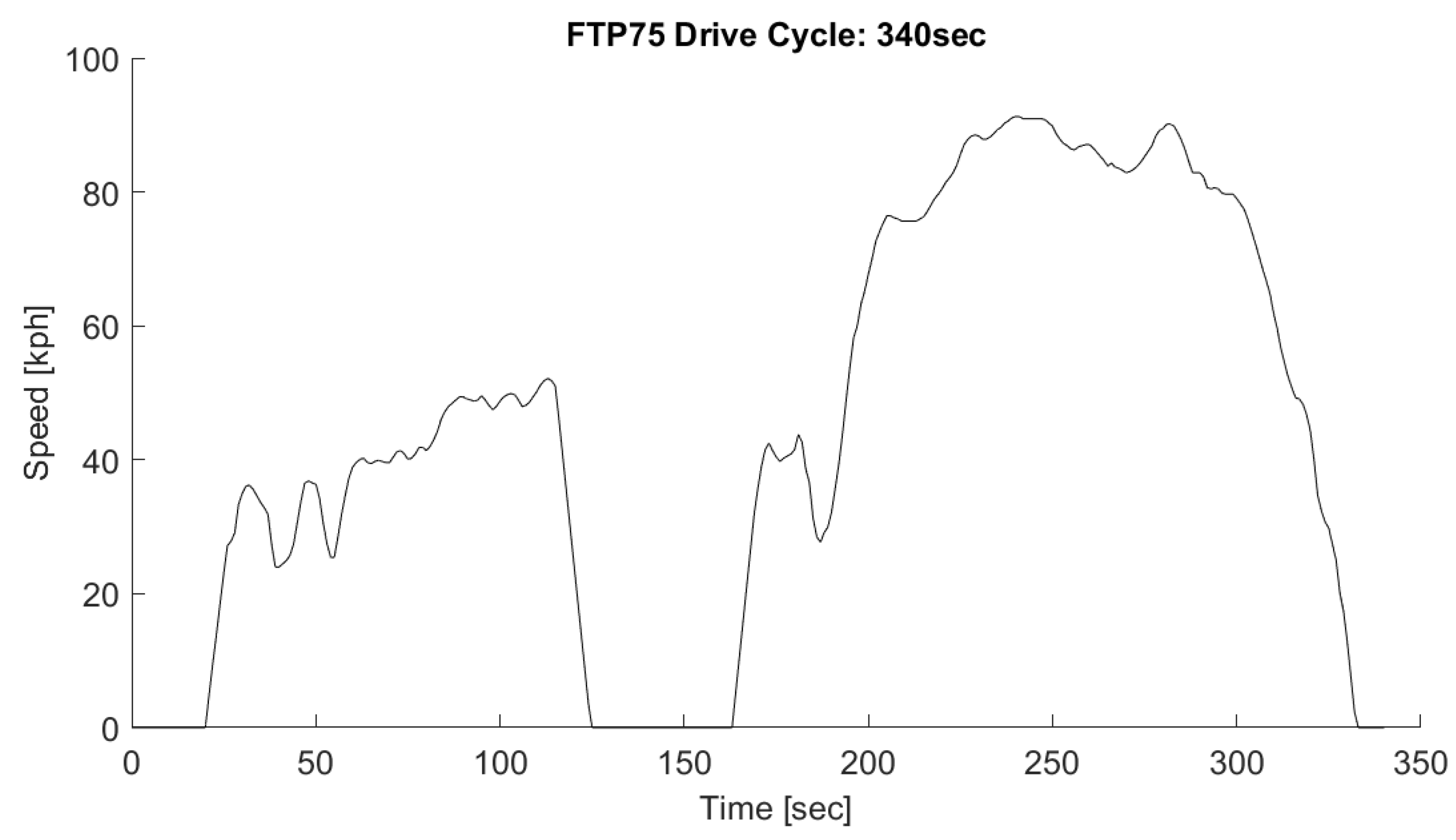
The overarching purpose of this paper is to support the collection of PEMFC experimental data under various drive cycles. A controller that is robust, consistent, and provides reference tracking with small errors will mitigate the controller’s contribution to variability in the experimental data. Since the driver controller will be implemented on actual hardware, having the computational resources to execute the controller on embedded hardware may be a nontrivial issue. High-performance microcontrollers are widely available and will be used in the eventual construction of the scale car to increase the chance that higher order controllers such as the ${\mathrm{H}}_{\infty }$ and Youla-H controllers can be used.

If the selected hardware is found to be insufficient, order reduction methods [13] will be used in order to simplify the controller transfer function. There are a wide variety of order reduction methods and the exploration of such is outside the scope of this paper. Order reduction will only be undertaken if necessary. If the required degree of reduction in order to implement the controller significantly reduces the system performance, then alternate controllers with lower order will be selected, such as the PI or Youla controllers.

In addition to managing the complexity of the implemented controller, it must be converted from a continuous-time representation to a discrete-time representation. The discretization may further introduce performance losses depending on the method used and the computational speed of the hardware. These implementation details may be the subject of future work if implementation is found to be nontrivial.

5. Results

Table 1 shows the system and controller parameters for the full-scale and scaled-down systems. The full-scale values are representative of an actual hydrogen-powered EV. The five independent scalings are chosen such that the scaled values approximate the expected values for an actual scaled-down EV. Other scalings are calculated in accordance with the scaling system described in the System Modeling section.

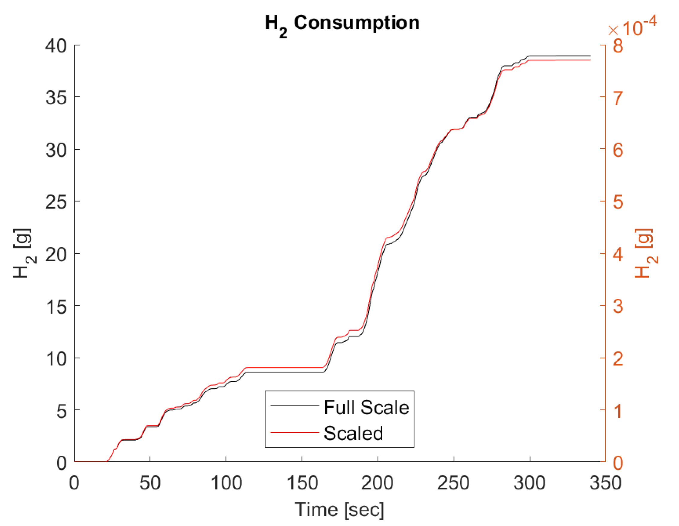
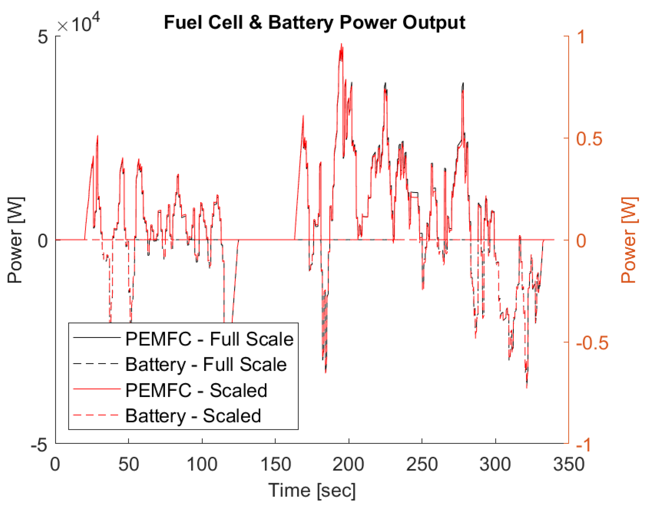
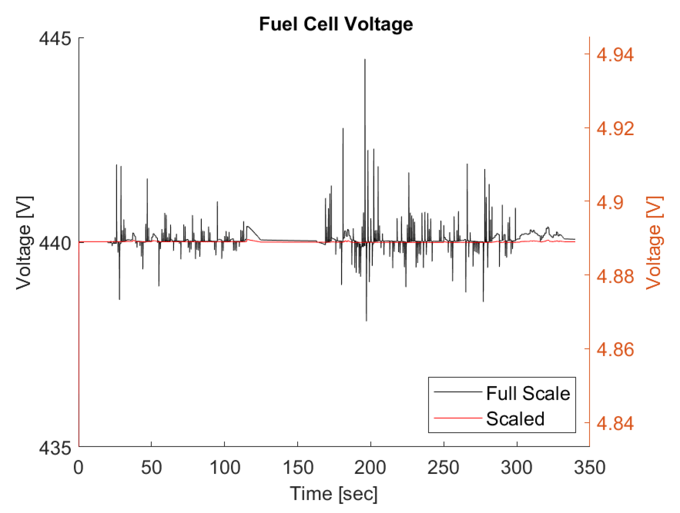
5.1. Fuel Cell Scaling Results

To verify that the scaling system will be useful for correlating experimental data, the hydrogen consumption, power requirements, and voltage behavior shown on the full nonlinear model need to have a ratio equal to the relevant scaling factors when comparing the full-scale and scaled simulation results. The hydrogen consumption and power requirements both scale by the energy scaling $S_E$, and the voltage by $S_V$, which are two of the independent scaling factors. For simplicity, these comparisons will be made on the system using the PI driver controller.

The primary goal of this work is to support research into efficient energy management in an EV, quantified by the total consumption of $H_2$ gas during the drive cycle. Future work will explore the energy management strategies themselves. Within the scope of this paper, the simple strategy utilized is that the fuel cell will provide all power to the motor up to the limit of what it can provide, after which the battery will supplement power to the motor. During regenerative braking, all power coming from the motor goes into the battery. The battery state-of-charge (SOC) is allowed to float for the purposes of this simple validation scenario.

Figure 16 shows the full-scale $H_2$ consumption on the left axis, and the scaled $H_2$ consumption on the right axis. The axes are scaled such that the right axis equals the left axis times the energy scaling factor $S_E$ so that the two curves can accurately be compared graphically.

The total consumptions for executing the full-scale and scaled-down drive cycles are 38.9 g and 770 $\mathrm{\mu }$g, respectively. As can be seen in Figure 16, the scaled consumption is close to the full-scale consumption but not exactly due to nonlinearities. The final consumption of 770 $\mathrm{\mu }$g is only 1.05% below the theoretical value of $S_{E}38.9$ g = 779 $\mathrm{\mu }$g.

Figure 17 shows the power output of both the fuel cell and the battery at full-scale and scaled-down cycles, similar with the axes scaled so that a graphical comparison is meaningful. With the simple energy management strategy used, the fuel cell provides all positive power since the power required never exceeds the maximum output of the fuel cell, while all negative power is absorbed by the battery. The alignment between the power curves of the fuel cell and battery between both scaling scenarios indicates that the scaling system worked correctly.

Figure 18 shows the voltage output of the fuel cell, with the right axis scaled by the voltage scaling $S_V$ so that the curves can be compared.

The average voltage output aligns between the full-scale and scaled-down scenarios, which is as expected since the number of cells in the fuel cell stack is directly scaled by $S_V$. However, as expected from the discussion in the Electrical Scaling section, the voltage transients are larger at full-scale. The scaled voltage transients not being fully representative in the scale system is an acceptable tradeoff as long as the total $H_2$ consumption is comparable.

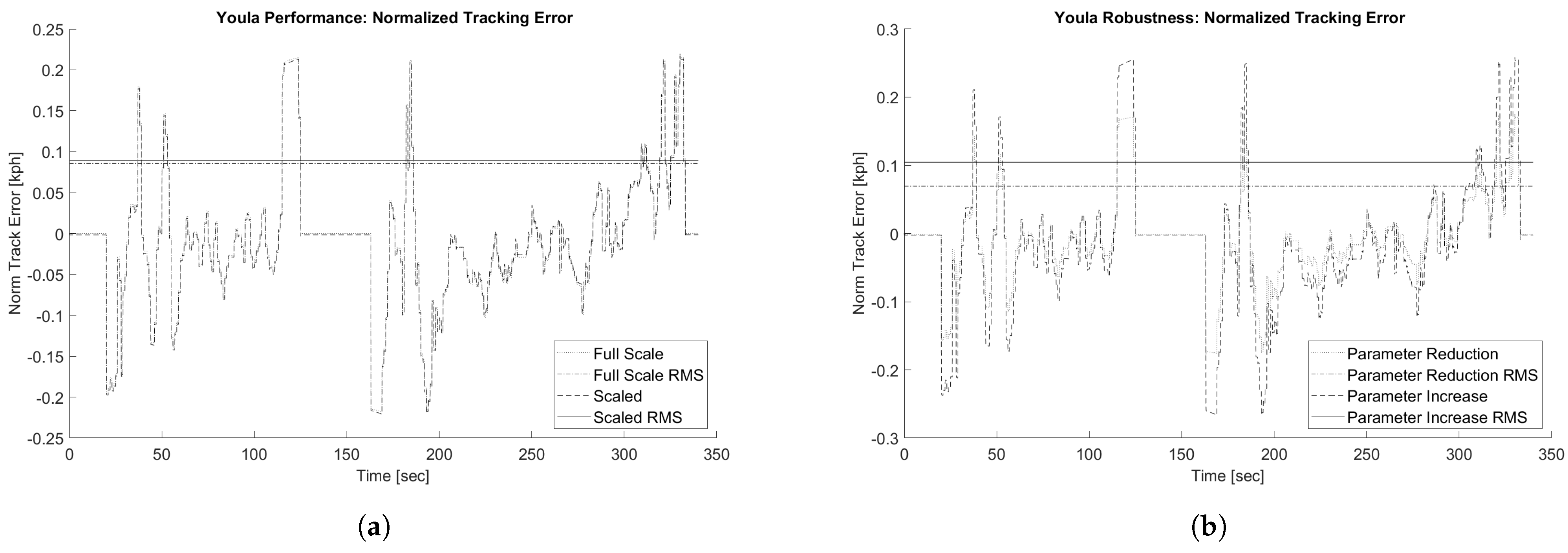
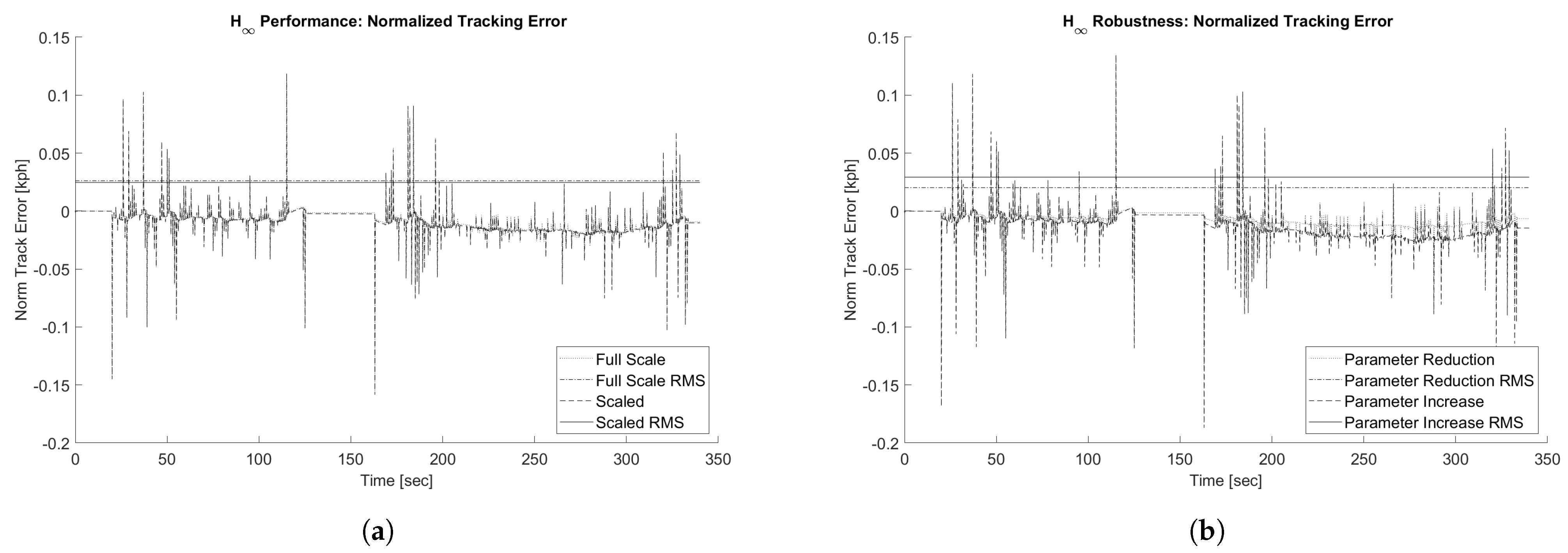
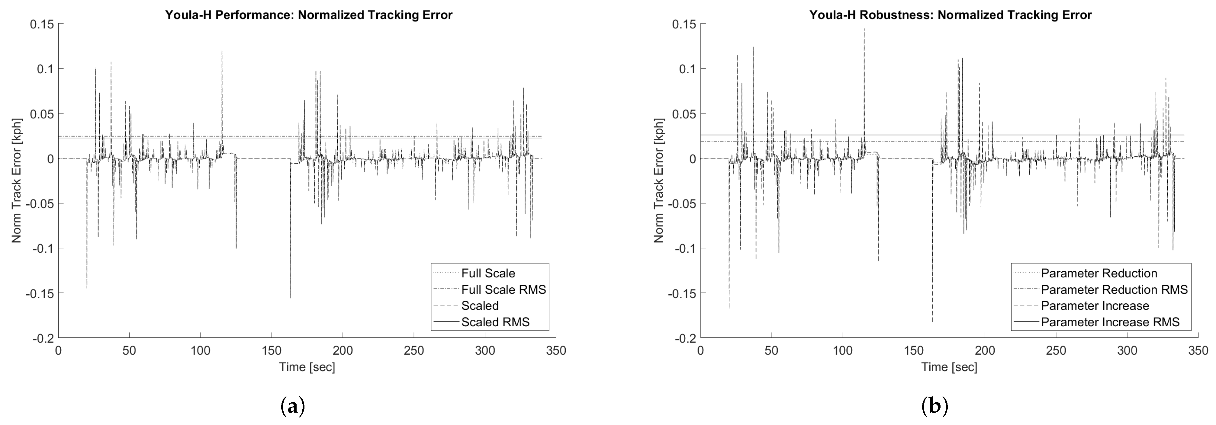
5.2. Tracking Error Results

To compare performance between controllers, reference speed tracking is evaluated on the nonlinear system model with the first 340 s of the FTP75 drive cycle as the input, as shown in Figure 19. For clarity, subsequent figures will show only the normalized tracking error rather than the full drive cycle velocities, as the errors are very small relative to the absolute speed.

All tracking error figures show the normalized tracking error, representing the difference between vehicle and drive cycle reference speeds normalized to full-scale speed values. The tracking errors on the scaled simulations are divided by the length scaling. The root mean square (RMS) error values are also plotted.

To evaluate the controller’s robustness against plant model uncertainty, two additional simulation scenarios are used. The ‘Parameter Reduction’ and ‘Parameter Increase’ scenarios, respectively, reduce and increase the actual plant mass, motor friction, motor inertia, tire radius, and gear ratio by 20% compared to the linear plant $G_P$ that the controllers are designed on.

Figure 20, Figure 21, Figure 22 and Figure 23 plot the normalized tracking errors of the PI, Youla, ${\mathrm{H}}_{\infty }$, and Youla-H controllers during the FTP75 drive cycle for the full-scale, scaled, and parameter variation scenarios. All tracking errors are low, with a maximum observed error of only 0.24 kph throughout the scenarios.

The Youla controller sees periods of consistent error, as it is not able to integrate away ramping input error fast enough, whereas the other controllers quickly recover. The ${\mathrm{H}}_{\infty }$ tracking performance tends to undershoot the drive cycle from 200 s onward. One of the modest improvements of the Youla-H controller over the initial ${\mathrm{H}}_{\infty }$ controller is that Youla-H removes this undershoot, which can be observed by comparing Figure 22 and Figure 23.

Table 2. Maximum absolute tracking errors.

Max Error [kph]	PI	Youla	${\mathbf{H}}_{\mathit{\infty }}$	Youla-H
Full-Scale	0.203	0.220	0.157	0.156
Scaled	0.203	0.221	0.158	0.156
Scaled-Reduction	0.164	0.179	0.135	0.134
Scaled-Increase	0.241	0.264	0.187	0.184

shows the maximum absolute tracking errors for the controllers across scenarios, while

Table 3. Root-Mean-Square Tracking Errors.

RMS Error [kph]	PI	Youla	${\mathbf{H}}_{\mathit{\infty }}$	Youla-H
Full-Scale	0.045	0.086	0.026	0.024
Scaled	0.045	0.089	0.025	0.023
Scaled-Reduction	0.037	0.069	0.020	0.019
Scaled-Increase	0.054	0.105	0.029	0.026

shows the root-mean-square (RMS) tracking errors.

The Youla controller has the highest maximum and RMS errors, followed by the PI controller, then ${\mathrm{H}}_{\infty }$, then Youla-H. The Youla-H controller has only a slight improvement in maximum absolute error over ${\mathrm{H}}_{\infty }$, but percentage-wise has a more modest improvement in RMS error. This is due to the ${\mathrm{H}}_{\infty }$$T\left(0\right)$ being slightly less than 1.0, and so the ${\mathrm{H}}_{\infty }$ controller has small but persistent undershoot during portions of the drive cycle, whereas the Youla-H controller removes this bias.

5.3. Noise and Disturbance Rejection

To simulate sensor noise on vehicle speed estimation, sinusoidal noise is injected into the controller input with an amplitude of 0.1 kph and a frequency of 2000 rad/s. This frequency is selected as it is where the Youla and ${\mathrm{H}}_{\infty }$ controllers have a similar order of magnitude of noise attenuation. For all controllers, this creates very minimal oscillations in vehicle speed and tracking error, as the frequency is too high to affect vehicle dynamics. However, there are large differences in the control signal, as shown in Figure 24.

Due to the PI controller’s Y transfer function staying at a high gain in high frequencies, it will jitter with any measurement noise at any frequency, whereas the other controllers will significantly attenuate this noise.

5.4. Controller Metrics

The controller performance metrics are aggregated in

Table 4. Controller performance metrics.

Metric	PI	Youla	${\mathbf{H}}_{\mathit{\infty }}$	Youla-H
Max Error Nominal [kph]	0.203	0.221	0.158	0.156
Max Error Reduced Param %	−19.0%	−19.0%	−14.7%	−14.4%
Max Error Increased Param %	18.6%	20.6%	18.0%	17.6%
RMS Error Nominal [kph]	0.045	0.089	0.025	0.023
RMS Error Reduced Param %	−19.2%	−22.4%	−18.2%	−16.4%
RMS Error Increased Param %	18.1%	16.9%	18.2%	15.6%
M2 Margin	1.000	0.866	0.937	0.937
Noise Std. Dev. [Nm]	0.0071	0.0005	0.0005	0.0005
Noise Max [Nm]	0.0142	0.0043	0.0063	0.0063

.

The Youla-H controller has the best performance across controllers. It has the longest design process but scales precisely with plant parameters and is adaptable to other plant dynamics. Once the design process is complete, the scaling system calculates this optimal controller without requiring user input.

While the PI controller has the best stability margins (M2, gain, and phase), its actual performance under requirements requiring robustness, in particular, its sensor noise attenuation, is lower than the ${\mathrm{H}}_{\infty }$ and Youla-H controllers due to the shape of the PI controller’s closed-loop transfer functions.

6. Conclusions

This paper has presented a hydrogen fuel cell and electric vehicle (EV) power train model, along with a method for scaling the model to arbitrary sizes and characteristics in support of energy management research on actual scaled test vehicles in order to extrapolate results to full-size vehicles. In addition, various control methods were examined for the driver control aspect of the model and were integrated into the scaling system in order to provide consistent and meaningful simulation results.

The proportional–integral (PI) controller gains were scaled to provide consistent normalized tracking results. The Youla controller was derived from the vehicle parameters and so had inherent dynamic similitude without requiring additional design time. The ${\mathrm{H}}_{\infty }$ controller required a scaling factor on one of its weighting functions but provided robust and high-performance control. The hybrid Youla and ${\mathrm{H}}_{\infty }$ (Youla-H) controller improved on this performance further with less design time than full ${\mathrm{H}}_{\infty }$ tuning and with the inherent ability of the scale, same as the standalone Youla controller. The PI method suffered from high susceptibility to noise, while the other controllers attenuated its effects. Overall, the hybrid Youla-H method achieved the best robustness and performance while being easy to scale with model parameters.

The performance of this powertrain model and of the controllers were nearly identical when simulated on the full-scale and scaled-down nonlinear models. This framework will thus provide a good foundation for research into energy management strategies.

References

1. Yadav, S.; Assadian, F. Robust Energy Management of Fuel Cell Hybrid Electric Vehicles Using Fuzzy Logic Integrated with H-Infinity Control. Energies 2025, 18, 2107. [Google Scholar] [CrossRef]
2. Hyundai Motor Company. The All-New NEXO. Available online: https://www.hyundai-n.com/en/models/rolling-lab/n-vision-74 (accessed on 30 May 2025).
3. Hyundai Motor Company. N Vision 74. Available online: https://www.hyundai.com/worldwide/en/eco/nexo/highlights (accessed on 30 May 2025).
4. Fathabadi, H. Combining a proton exchange membrane fuel cell (PEMFC) stack with a Li-ion battery to supply the power needs of a hybrid electric vehicle. Renew. Energy 2019, 130, 714–724. [Google Scholar] [CrossRef]
5. Petersheim, M.D.; Brennan, S.N. Scaling of hybrid-electric vehicle powertrain components for Hardware-in-the-loop simulation. Mechatronics 2009, 19, 1078–1090. [Google Scholar] [CrossRef]
6. Gao, Z. Scaling and bandwidth-parameterization based controller tuning. In Proceedings of the 2003 American Control Conference, Denver, CO, USA, 6 June 2003; pp. 4989–4996. [Google Scholar] [CrossRef]
7. Baek, W.; Song, B.; Song, H. Development of a Longitudinal Vehicle Controller via Hardware-in-the-Loop Simulation. In Proceedings of the ASME 2007 International Mechanical Engineering Congress and Exposition. Volume 16: Transportation Systems, Seattle, WA, USA, 11–15 November 2007; pp. 87–95. [Google Scholar] [CrossRef]
8. Qu, T.; Wang, Q.; Cong, Y.; Chen, H. Modeling driver’s longitudinal and lateral control behavior: A moving horizon control modeling scheme. In Proceedings of the 2018 Chinese Control And Decision Conference (CCDC), Shenyang, China, 9–11 June 2018; pp. 3260–3264. [Google Scholar] [CrossRef]
9. Bara’c, B.; Krpan, M.; Capuder, T. Modelling of PEM fuel cell for power system dynamic studies. IEEE Trans. Power Syst. 2024, 39, 3286–3298. [Google Scholar] [CrossRef]
10. Hariharan, K.S.; Senthil Kumar, V. A nonlinear equivalent circuit model for lithium ion cells. J. Power Sources 2013, 222, 210–217. [Google Scholar] [CrossRef]
11. Pritchard, P.J.; Mitchell, J.W. Fox and McDonald’s Introduction to Fluid Mechanics, 9th ed.; John Wiley & Sons: Hoboken, NJ, USA, 2015. [Google Scholar]
12. Assadian, F.; Mallon, K.R. Robust Control: Youla Parameterization Approach; John Wiley & Sons: Hoboken, NJ, USA, 2022. [Google Scholar]
13. Dehkordi, V.R.; Boulet, B. Robust controller order reduction. Int. J. Control 2011, 84, 985–997. [Google Scholar] [CrossRef]
Figure 1. System model architecture.
Energies 18 03126 g001
Figure 2. PEMFC low-level H control.
Energies 18 03126 g002
Figure 3. Battery model.
Energies 18 03126 g003
Figure 4. Example system.
Energies 18 03126 g004
Figure 5. Linear plant model.
Energies 18 03126 g005
Figure 6. H weighting functions.
Energies 18 03126 g006
Figure 7. Full-scale and scaled Bode magnitude and phase plots of the open-loop transfer function L for (a) PI controller; (b) Youla controller; (c) H controller; (d) Youla-H controller.
Energies 18 03126 g007
Figure 8. Bode magnitude plots of the closed-loop transfer functions T, S, and Y for (a) full-scale PI controller and (b) scaled PI controller.
Energies 18 03126 g008
Figure 9. Bode magnitude plots of the closed-loop transfer functions T, S, and Y for (a) full-scale Youla controller and (b) scaled Youla controller.
Energies 18 03126 g009
Figure 10. Bode magnitude plots of the closed-loop transfer functions T, S, and Y, and the inverse of the weighting functions 1 / W p , 1 / W d , and 1 / W u for (a) full-scale H controller and (b) scaled H controller.
Energies 18 03126 g010
Figure 11. Bode magnitude plots of the closed-loop transfer functions T, S, and Y for (a) full-scale Youla-H controller and (b) scaled Youla-H controller.
Energies 18 03126 g011
Figure 12. Y for all controllers.
Energies 18 03126 g012
Figure 13. T for all controllers at low frequencies.
Energies 18 03126 g013
Figure 14. S for all controllers at low frequencies.
Energies 18 03126 g014
Figure 15. Nyquist plots for (a) PI controller, (b) Youla controller, (c) H controller, and (d) Youla-H controller.
Energies 18 03126 g015
Figure 16. Hydrogen consumption over drive cycle.
Energies 18 03126 g016
Figure 17. Fuel cell and battery power output over drive cycle.
Energies 18 03126 g017
Figure 18. Fuel cell output voltage over drive cycle.
Energies 18 03126 g018
Figure 19. FTP75 drive cycle, reference velocity input for all controllers.
Energies 18 03126 g019
Figure 20. Normalized tracking errors for (a) PI controller, full-scale vs scaled and (b) PI controller with parameter variations.
Energies 18 03126 g020
Figure 21. Normalized tracking errors for (a) Youla controller, full-scale vs scaled and (b) Youla controller with parameter variations.
Energies 18 03126 g021
Figure 22. Normalized tracking errors for (a) H controller, full-scale vs scaled and (b) H controller with parameter variations.
Energies 18 03126 g022
Figure 23. Normalized tracking errors for (a) Youla-H controller, full-scale vs scaled and (b) Youla-H controller with parameter variations.
Energies 18 03126 g023
Figure 24. Actuator effort with noise on the scaled-down plant for (a) PI controller, (b) Youla controller, (c) H controller, and (d) Youla-H controller.
Energies 18 03126 g024