Article

Damping Characteristic Analysis of LCL Inverter with Embedded Energy Storage

State Grid Jiangsu Electric Power Co., Ltd., Research Institute, Nanjing 211103, China
*
Author to whom correspondence should be addressed.
Energies 2025, 18(12), 3127; https://doi.org/10.3390/en18123127 (registering DOI)
Submission received: 7 May 2025 / Revised: 2 June 2025 / Accepted: 3 June 2025 / Published: 13 June 2025
(This article belongs to the Topic Power System Dynamics and Stability, 2nd Edition)

Abstract

:
This paper investigates the system architecture and circuit topology of grid-connected inverters with embedded energy storage (EES), encompassing their modulation strategies and control methodologies. A mathematical model for an EES grid-connected inverter is derived based on capacitor current feedback control, from which the expression for the inverter’s output impedance is obtained. Building on this foundation, this study analyzes the influence of control parameters—such as the proportional coefficient, resonant coefficient, and switching frequency—on the inverter’s output impedance. Subsequently, the stability of single and multiple inverter grid-connected systems under various operating conditions is assessed using impedance analysis and the Nyquist criterion. Finally, the validity of the stability analysis based on the established mathematical model is verified through simulations conducted on the Matlab/Simulink platform, where models for both a single inverter and a two-inverter grid-connected system are constructed.

1. Introduction

With the rapid expansion of renewable energy sources, the pressure from the fossil fuel crisis has been reduced. However, the widespread adoption of renewable energy has transformed the nature of traditional power systems, resulting in a dual trend: increased renewable energy penetration and a higher proportion of power electronic devices in the system [1,2,3]. Within modern power systems, the interplay between power electronic devices and the grid has made system stability more complex. A large presence of power electronic devices in the grid can often lead to broadband oscillations, which may hinder the stable operation of the grid-connected system [4]. For example, in 2009, a sub-synchronous oscillation occurred in a renewable energy grid system in Texas, USA, leading to the disconnection of many wind turbines [5]. Between 2012 and 2016, sub-synchronous oscillations repeatedly affected wind farms in Guyuan, Hebei Province, China, with oscillation frequencies between 4 and 10 Hz, posing a threat to the grid’s stable and safe operation [6,7]. In 2015, a sub-synchronous oscillation with a frequency of 34 Hz took place in the Hami region of Xinjiang, China, due to the integration of permanent magnet direct-drive turbines in a weak grid. This issue resulted in high-frequency oscillations caused by the connection of multiple renewable energy power plants to the grid through long-distance transmission lines [8,9,10].
Wide-range-frequency oscillations fundamentally differ from the instabilities observed in traditional power systems, making it challenging to apply the stability analysis methods used in traditional power systems to study the stability issues of systems characterized by the high penetration of renewables and a high proportion of power electronic devices. Consequently, the stability of such dual-high systems has become a current research hotspot both domestically and internationally. Among the components of these systems, grid-connected inverters, as crucial interface devices for new energy grid-connected power generation, have received widespread attention [11]. Common research methods for analyzing the stability of inverter systems include eigenvalue analysis and impedance analysis. The former involves establishing a state-space model based on the grid-connected system, linearizing the system’s state equations using the small signal method, and then determining the system’s stability by calculating the eigenvalues and eigenvectors of the state space. However, any changes in the system structure or control parameters necessitate re-establishing the system’s state equations, complicating the modeling process. With the integration of new energy sources, grid impedance varies widely, further complicating stability analysis and reducing the method’s generality [12,13]. Currently, the commonly used method is impedance analysis [14]. This approach divides the grid-connected inverter and the grid into two independent systems, modeling their impedances separately. Changes in the parameters of one system do not affect the model of the other, allowing for stability analysis based on impedance stability criteria. When grid impedance changes, there is no requirement to rebuild the model of the grid-connected inverter. This method is widely applicable, and many studies have employed it to perform detailed analyses of the stability of voltage source inverter–grid coupled systems, resulting in several valuable conclusions.
As a crucial interface device between new energy systems and the power grid, grid-connected inverters require appropriate filters to suppress switching harmonics generated by switching devices during operation, ensuring that the output grid-connected current meets harmonic requirements. The main types of filters are L-type and LCL-type. Under the same filtering effect, LCL-type filters offer lower costs and smaller sizes, making them commonly used [15,16]. However, LCL-type inverters exhibit resonance peaks, where the phase undergoes a −180° shift at the resonant frequency [17], making the system prone to resonance and instability. Therefore, damping of these resonance peaks is necessary [18]. Current damping methods are categorized into passive damping, which involves series or parallel resistors in the circuit [19], and active damping, which introduces state variable feedback control [20,21]. The literature [22,23] analyzes passive damping methods for LCL, LLCL, and LLCCL filters, comparing the suppression effects of the Rd damping method and the Rd-Cd hybrid resistor–capacitor passive damping method. The former can dampen resonance but affects the gain characteristics in the high-frequency range, reducing high-frequency harmonic attenuation. The latter, with the addition of capacitance, can dampen resonance without affecting high-frequency harmonic attenuation. Passive damping methods are simple and effective but introduce losses. In weak grids, when grid impedance varies widely, these methods cannot adjust damping levels in a timely manner, limiting their suppression effectiveness. Active damping methods, on the other hand, do not introduce additional losses and offer more flexible damping implementation. Currently, there are multiple active damping methods, mainly divided into two approaches: one that does not require additional sensors, achieving damping through grid-connected current feedback or filter parameter estimation; and another that requires additional sensors, feeding back electrical quantities such as voltage or other currents to achieve virtual damping control. The literature [24] examines the core principles of active damping methods, demonstrating the feasibility of control techniques, including inverter-side and grid-side current feedback. The literature [25] proposes an active damping control method based on a band-pass filter, which does not require additional sensors and analyzes the damping effects of introducing the band-pass filter at different locations. The literature [26] proposes an improved active damping control method based on traditional grid-connected current feedback active damping, expanding the frequency range of positive damping. The literature [27] analyzes the damping characteristics and parameter selection based on capacitor current feedback under PI control. The literature [28] proposes an improved active damping method using differential feedback of the filter capacitor voltage, achieving resonance peak suppression without affecting filter performance. In summary, the most widely used method is active damping based on proportional feedback of capacitor current, which is equivalent to the passive damping method of paralleling a resistor across the capacitor. This method can provide virtual resistance for damping, and proportional feedback is easy to implement without introducing additional losses. The above comparisons of different methods are also presented in the following Table 1.
In recent years, the modular multilevel converter with embedded energy storage has emerged as a significant development direction in storage transmission. In this configuration, battery energy storage units are decentralized and integrated into the submodules within the converter arms, offering advantages such as multi-dimensional coordination and rapid response. However, to date, there has been a lack of relevant literature analyzing its impedance characteristics. To address these concerns, this paper studies this type of converter’s characteristics and the contributions are as follows:
(1)
The impedance model of BESS-MMC has been established, where the control and grid system parts are considered, which is realized through a Quasi-Proportional–Resonant (QPR) controller.
(2)
The key factors influencing the inverter’s impedance and its stability characteristics are investigated, and the recommendations for enhancing stability are also provided.
The organization of this paper is as follows: Section 2 introduces the operating principle of an LCL inverter with embedded energy storage, Section 3 analyzes the stability mechanism, Section 4 conducts simulation verifications, and Section 5 concludes the paper.

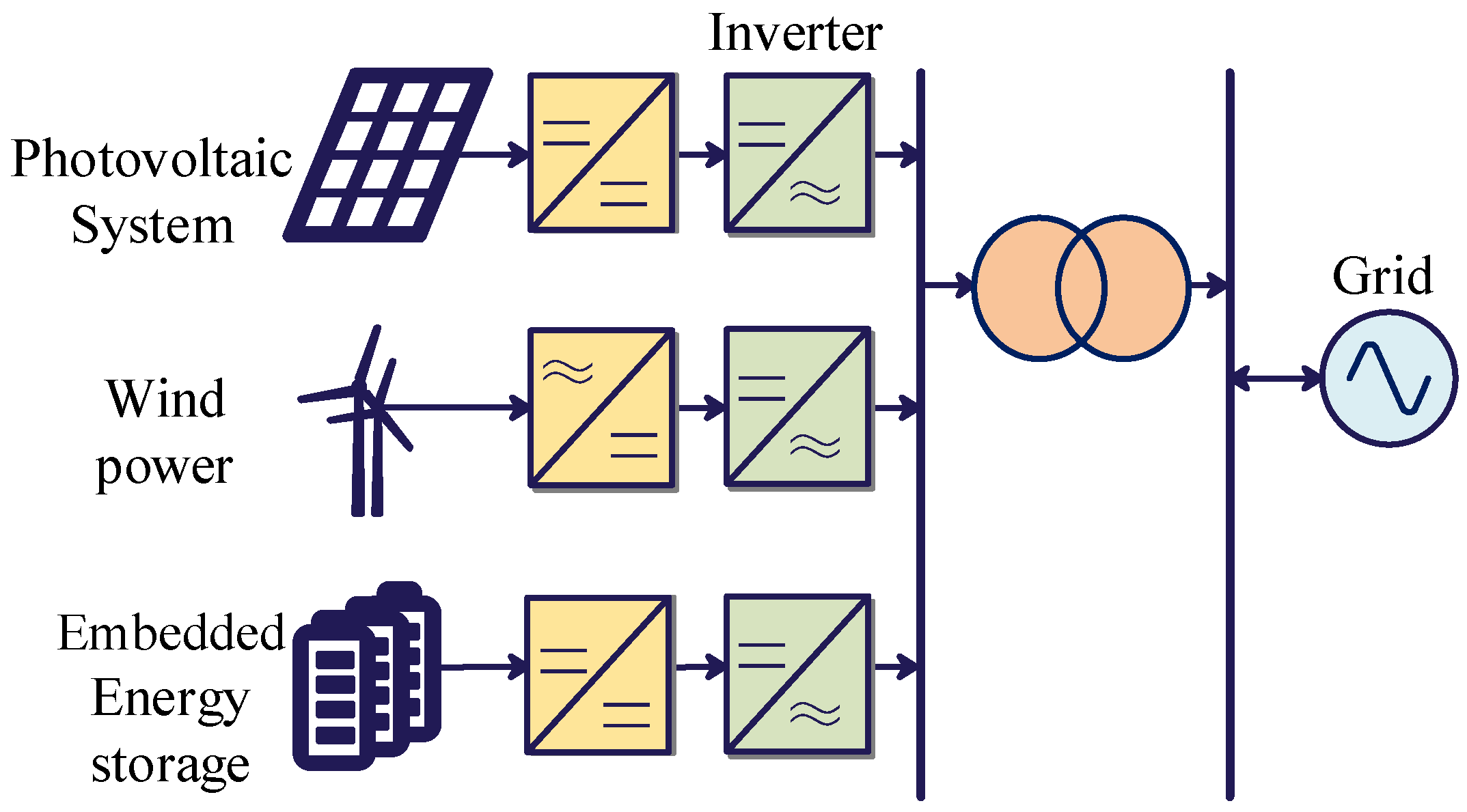
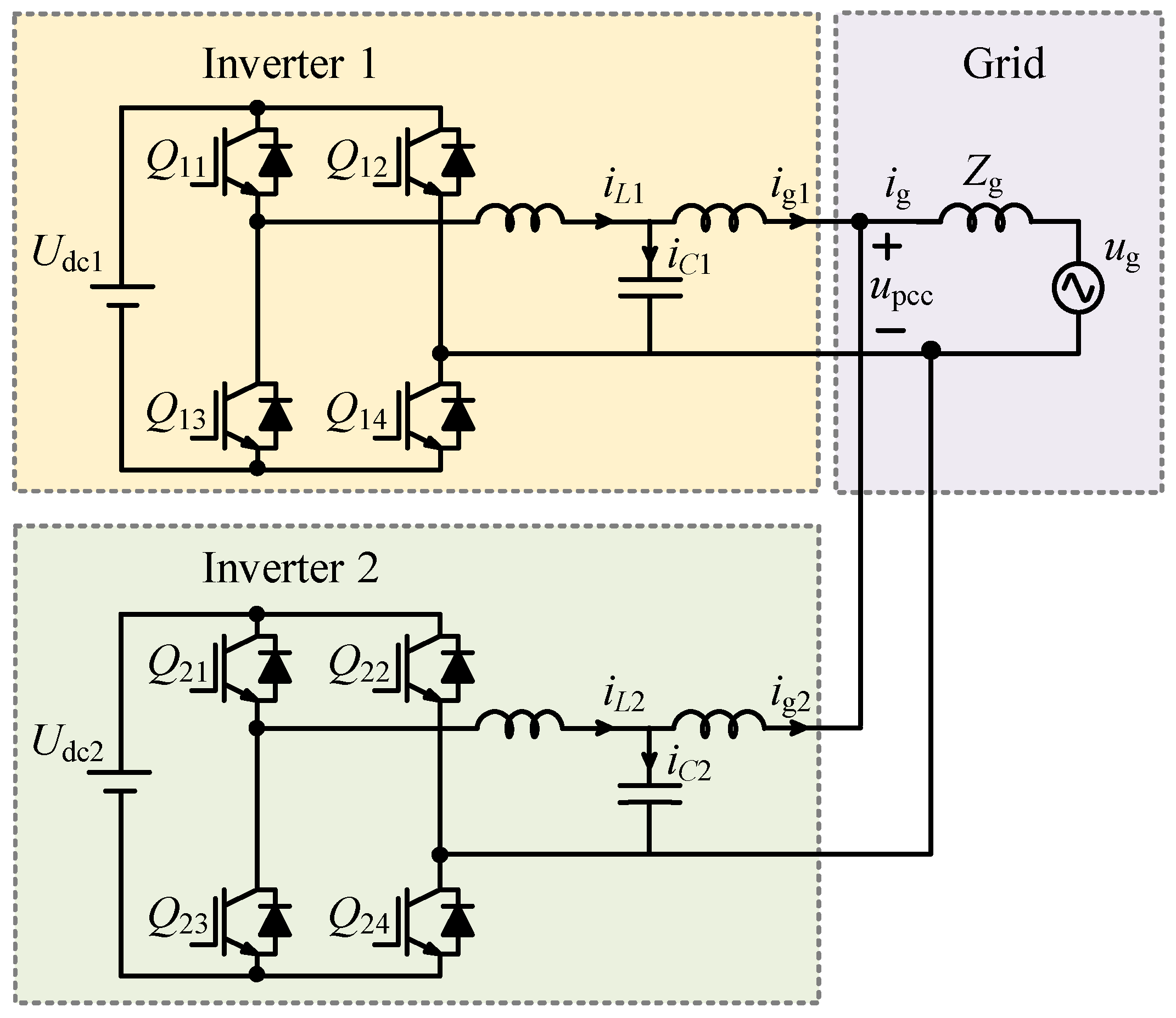
2. Operating Principle of LCL Inverter with Embedded Energy Storage

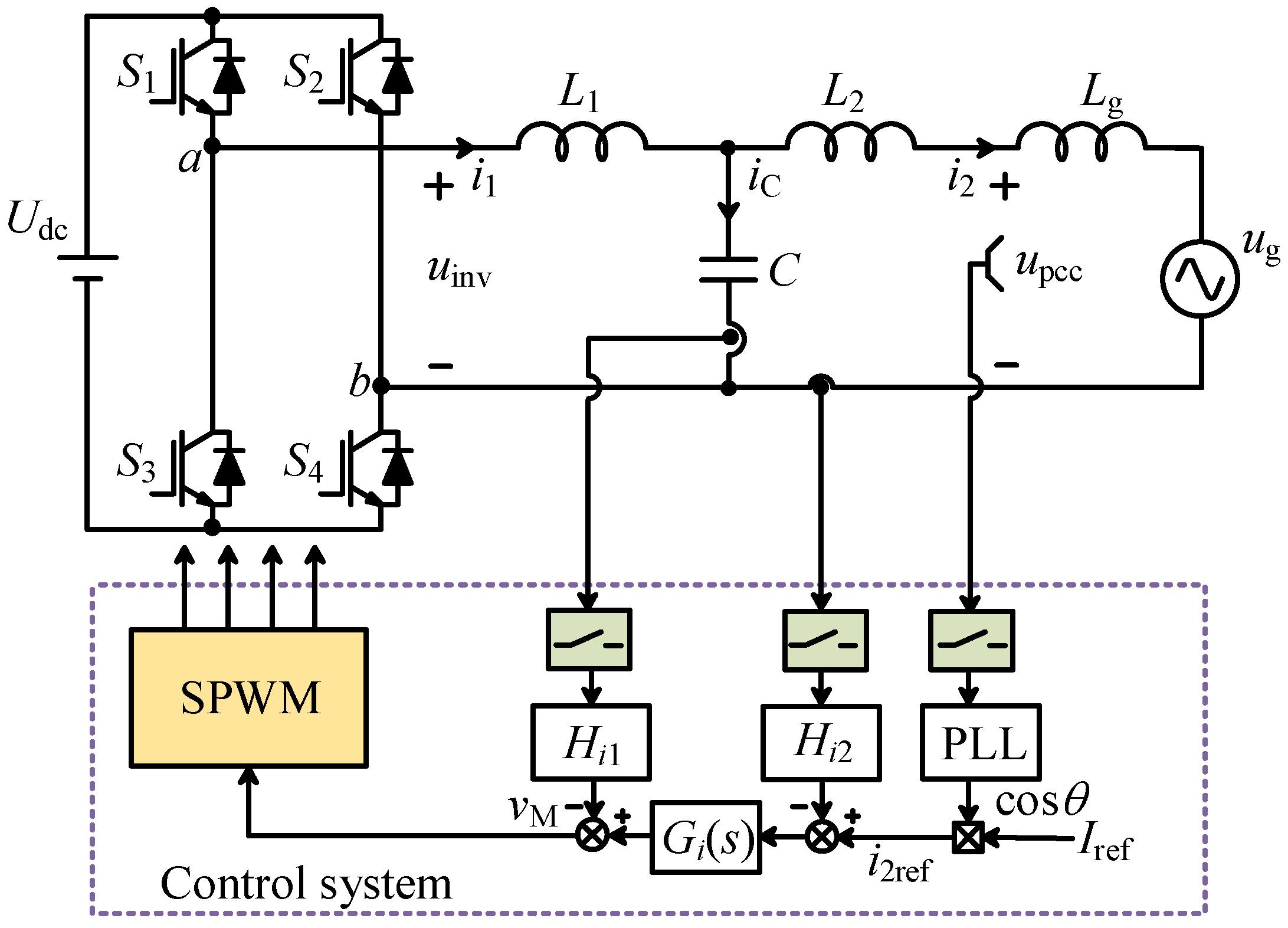
2.1. System Structure and Control Strategy

In analyzing the characteristics of Modular Multilevel Converters (MMCs), common assumptions are made to simplify the models and highlight the key phenomena. These include assuming ideal switching devices (neglecting losses and delays), a constant DC-side voltage, balanced capacitor voltages across sub-modules, negligible circulating currents, linear system behavior in steady-state or small signal analyses, negligible parasitic parameters, and steady-state operating conditions. These assumptions provide a foundational framework, though their application may require adjustments based on specific system needs and operational contexts.
The topological structure of a photovoltaic–wind complementary power generation system equipped with BESS-MMC is shown in Figure 1. It mainly consists of photovoltaic panels, wind turbines, energy storage batteries, grid-connected inverters, transformers, and other components. The relevant new energy sources and the BESS-MMC system adopt a grid-side inductor current feedback control strategy and are connected to the grid through an LCL-type grid-connected inverter.
Figure 2 illustrates the circuit and control diagram of a single-phase grid-connected inverter for embedded energy storage when digital control is employed. S1S4 represent the switching devices. L1 and L2 represent the inductors on the inverter and grid sides, respectively. Lg is the inductive grid impedance, and C is the filter capacitor. Udc is the DC-side voltage, ug is the grid voltage, uinv is the output voltage of the inverter, upcc is the voltage at the point of common coupling (PCC) between the inverter and the grid, i1 is the inductor current on the inverter side, iC is the filter capacitor current, and i2 is the grid-side current. Hi1 and Hi2 are the feedback coefficients for the capacitor current and the grid current sampling, respectively, and Gi(s) is the current regulator.
Firstly, the phase of the voltage at the point of common coupling is obtained by the Phase-Locked Loop (PLL) to ensure that the grid-connected current is in phase with the voltage. Iref is the amplitude of the reference current, and the current regulator is used to make the output grid-connected current track the reference current i2ref. In addition, to mitigate the resonance of the LCL filter, the Capacitor Current Feedback Active Damping (CCF-AD) control method is utilized. The feedback is applied to the output of the current regulator to obtain the modulation wave vM, which is then used to generate pulse signals through the modulation process to drive the switching devices.
The proper selection of a current regulator ensures that the output grid-connected current complies with the grid connection standards. Currently, commonly used current regulators in engineering include the Proportional–Integral (PI) controller and the Proportional–Resonant (PR) controller, and the Quasi-Proportional–Resonant (QPR) controller. Due to its excellent performance and simple control structure, the PI controller is widely used in practical engineering applications. However, it can only achieve zero steady-state error tracking for DC quantities, so it is often used in the dq coordinate system. The ideal PR controller has infinite gain at the fundamental frequency, but it is difficult to adapt to grid frequency fluctuations in practical engineering applications. The QPR controller, on the other hand, has better robustness than the PR controller and can adapt to grid frequency fluctuations, achieving nearly zero steady-state error tracking for AC quantities. It is often used in the αβ coordinate system. The Bode plots of these two controllers are shown in Figure 3. To conduct a quantitative analysis, we added the frequency drift tolerance comparison based on 0 dB-cross bandwidth, namely, the bandwidth covered 0 dB. It can be seen from Figure 3 that the frequency drift tolerance of QPR control is 43 rad/s, while PR control is only 7 rad/s, thus, the frequency drift tolerance of QPR control is about 6 times of PR control.
In summary, this paper selects the Quasi-Proportional–Resonant (QPR) controller, whose expression is given by
G i ( s ) = K p + 2 K r ω i s s 2 + 2 ω i s + ω 0 2
where Kp and Kr represent the proportional coefficient and the resonant coefficient, respectively; wi is the bandwidth of the resonant term; and w0 is the fundamental angular frequency.

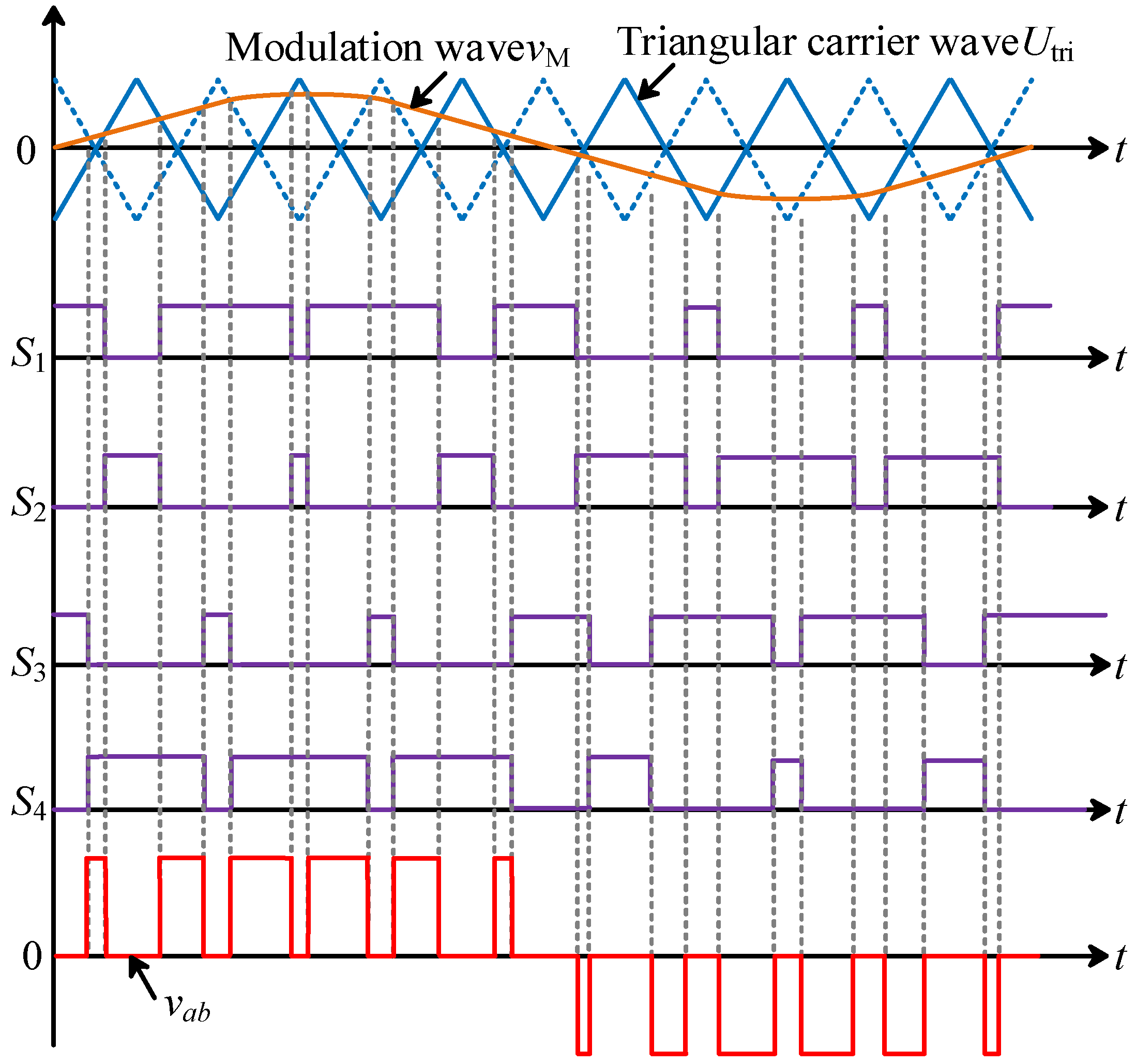
2.2. Modulation Strategy

The main circuit of the inverter consists of a DC power supply, an inverter bridge, and a filter. In this paper, the inverter adopts unipolar double frequency sinusoidal pulse width modulation (SPWM). The inverter bridge is composed of IGBT switches and antiparallel diodes. The schematic diagram of unipolar double frequency modulation is shown in Figure 4, where vM represents the modulation wave, ±Utri represent the triangular carrier waves, S1 and S2 are switches on the same leg, and S3 and S4 are switches on the other leg. The pulse signals for the left leg are obtained by comparing vM with Utri, and the pulse signals for the right leg are obtained by comparing vM with −Utri. The specific process is as follows: When vM > Utri, S1 is turned on and S2 is turned off; when vM < Utri, S1 is turned off and S2 is turned on. Similarly, when vM > −Utri, S3 is turned off and S4 is turned on; when vM < −Utri, S3 is turned on and S4 is turned off. From the schematic diagram, it can be seen that during the positive half-cycle of the modulation wave, the voltage vab between the legs has two levels: +Udc and 0. Similarly, during the negative half-cycle of the modulation wave, the voltage vab between the legs also has two levels: −Udc and 0. The frequency of vab is twice that of the triangular carrier wave. According to the literature [27], the Fourier series expression for the inverter output voltage vab under unipolar double frequency modulation is given by
v a b ( t ) = M U d c sin ω 0 t + 4 U d c π m = 2 , 4 , n = ± 1 , ± 3 , ± J n ( m M π / 2 ) m cos m π 2 sin ( m ω sw t + n ω 0 t )
where M denotes the modulation index, w0 represents the fundamental angular frequency, ωsw is the angular frequency of the triangular carrier wave, m and n are the multiples of the frequencies of the triangular carrier wave and the modulation wave, respectively, and Jn(x) is the Bessel function, expressed as
J n ( x ) = k = 0 ( 1 ) k k ! k + n ! x 2 2 k + n

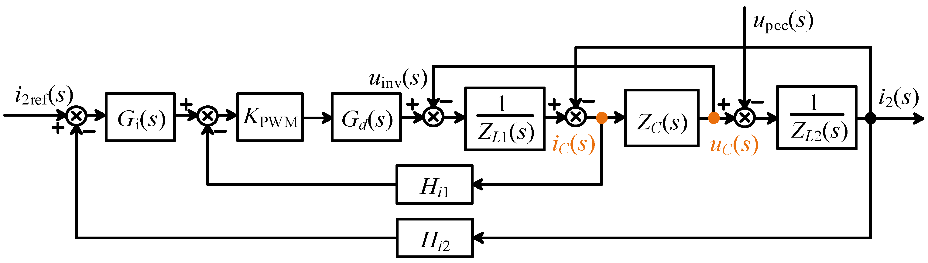
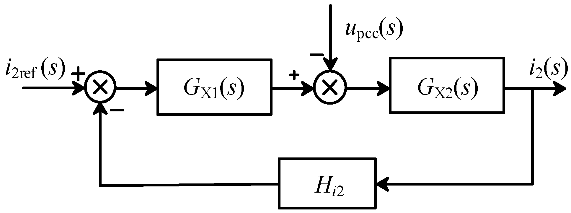
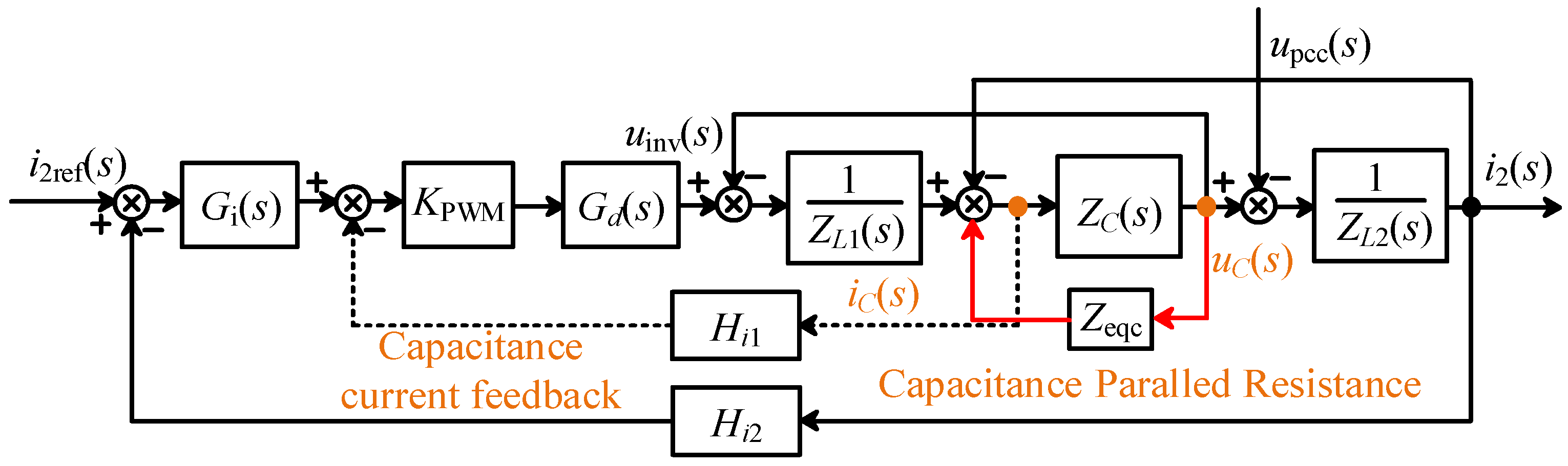
2.3. Mathematical Model

Based on the circuit and control structure of the embedded energy storage LCL grid-connected inverter shown in the figure, the mathematical model of the single-phase LCL grid-connected inverter is derived, as illustrated in Figure 5.
Where ZL1, ZC, and ZL2 represent the impedances corresponding to the inverter-side inductance, filter capacitor, and grid-side inductance, respectively. KPWM is the transfer function from the modulation wave to the inverter output voltage uinv. Gd(s) accounts for the one-sample calculation delay and the 0.5-sample modulation delay introduced by digital control, with its expression given as
G d ( s ) = e 1.5 s T s
Through block diagram transformation, Figure 5 can be further simplified into Figure 6. The expressions for GX1(s) and GX2(s) are presented in Equations (5) and (6), respectively.
G X 1 ( s ) = K PWM G d ( s ) G i ( s ) s 2 L 1 C + s C H i 1 K PWM G d ( s ) + 1
G X 2 ( s ) = s 2 L 1 C + s C H i 1 K PWM G d ( s ) + 1 s 3 L 1 L 2 C + s 2 L 2 C H i 1 K PWM G d ( s ) + s ( L 1 + L 2 )
As shown in Figure 6, the system’s loop gain can be expressed as:
T ( s ) = G X 1 ( s ) G X 2 ( s ) H i 2 = H i 2 K PWM G i ( s ) s 3 L 1 L 2 C + s 2 L 2 C H i 1 K PWM + s ( L 1 + L 2 ) = H i 2 K PWM ( K p + 2 K r ω i s / s 2 + 2 ω i s + ω 0 2 ) s 3 L 1 L 2 C + s 2 L 2 C H i 1 K PWM + s ( L 1 + L 2 )
Therefore, the grid-connected current i2(s) can be expressed as:
i 2 ( s ) = 1 H i 2 T ( s ) 1 + T ( s ) i 2 ref ( s ) G X 2 ( s ) 1 + T ( s ) u p c c ( s ) = i s ( s ) u p c c ( s ) Z o ( s )
The first part, is(s), in Equation (8) represents the equivalent ideal current source of the grid-connected inverter, while the second part, Zo(s), denotes the output impedance of the inverter, which can be expressed as:
Z o ( s ) = 1 + T ( s ) G X 2 ( s )

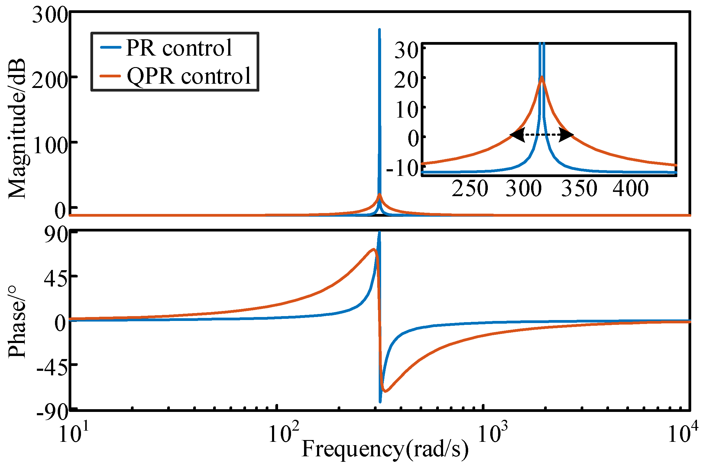
2.4. Impedance Characteristic Analysis

By substituting Equations (6) and (7) into Equation (9), the output impedance expression of the inverter using the CCF-AD control method is derived as
Z o ( s ) = s 3 L 1 L 2 C + s 2 L 2 C H i 1 K PWM G d ( s ) + s ( L 1 + L 2 ) + K PWM G d ( s ) G i ( s ) H i 2 s 2 L 1 C + s C H i 1 K PWM G d ( s ) + 1 = s 3 L 1 L 2 C + s 2 L 2 C H i 1 K PWM e 1.5 s T s + s ( L 1 + L 2 ) + K PWM e 1.5 s T s G i ( s ) H i 2 s 2 L 1 C + s C H i 1 K PWM e 1.5 s T s + 1
From Equation (10), it can be observed that the output impedance of the inverter is related to the circuit parameters, control parameters, sampling coefficients, capacitor current feedback coefficients, and switching frequency. It can also be noticed that the time delay appears in the equation, where the delays may reduce the system’s stability margin and shrink the stable operating region of the system.
Below, we will analyze the influence of each parameter on the output impedance. The parameters of the circuit are provided in Table 2.
(1)
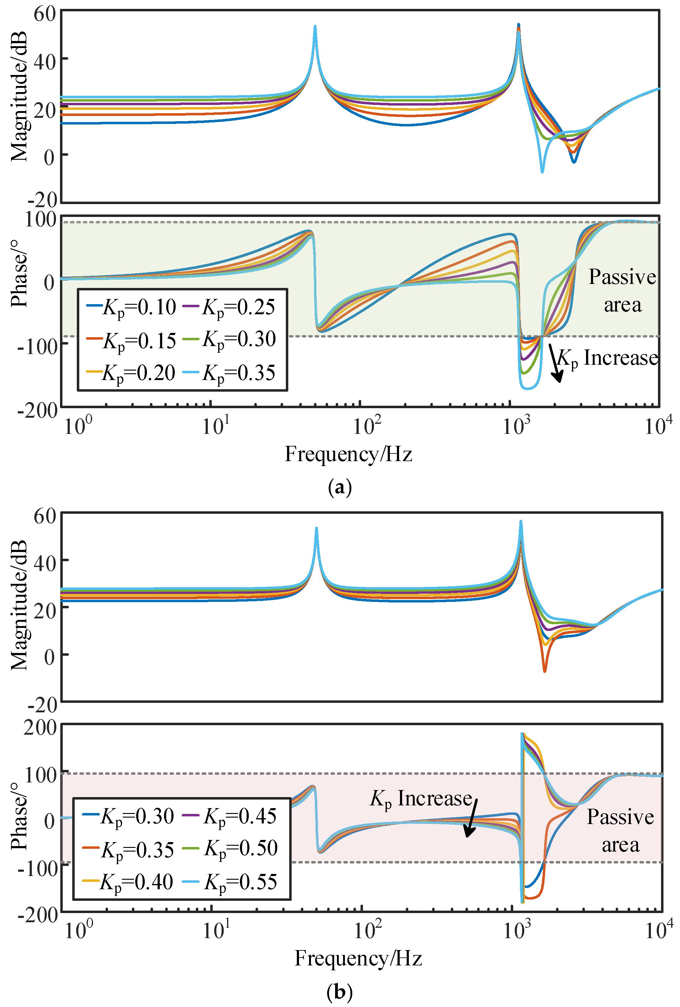
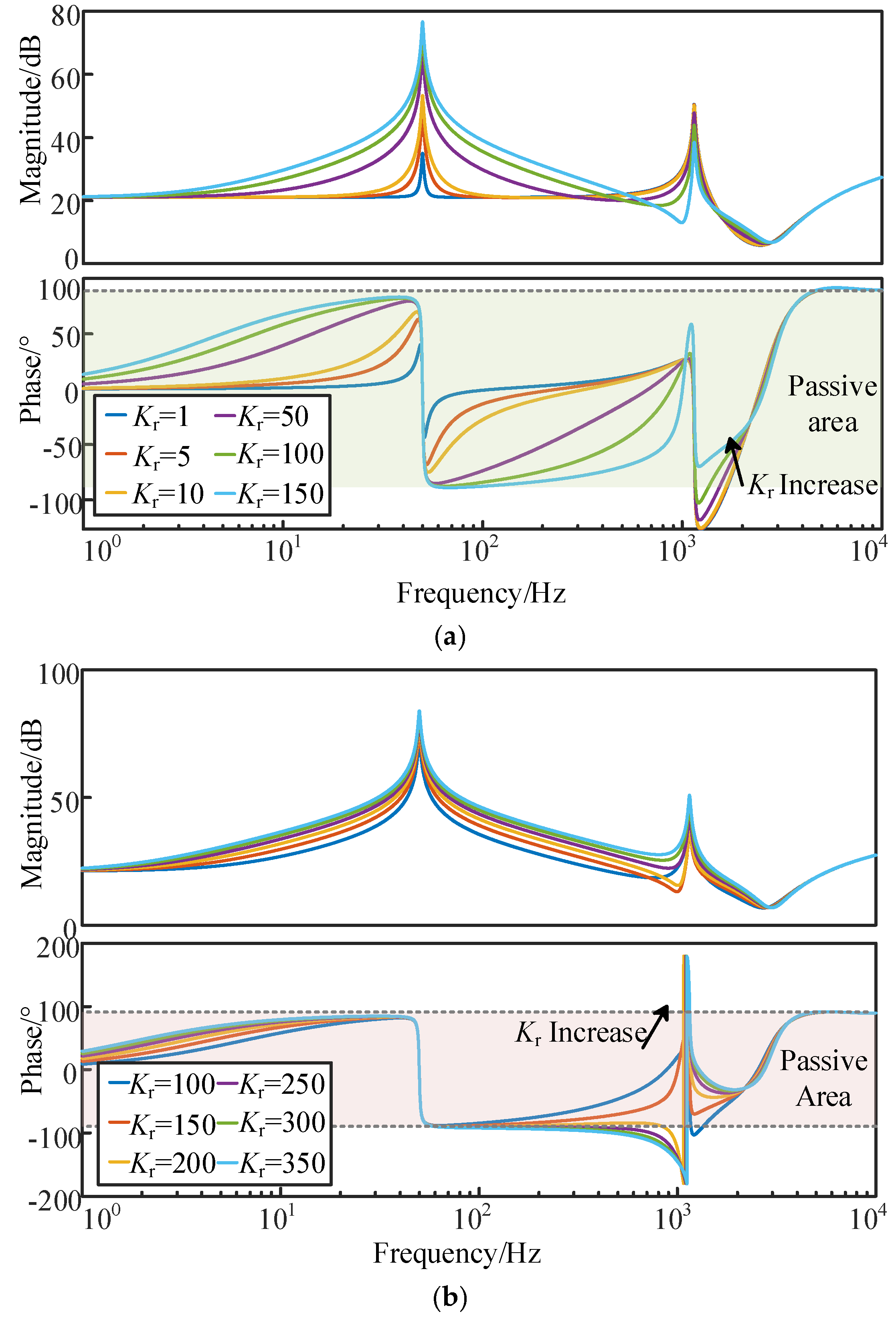
Influence of Control Parameters
The output impedance of the inverter is influenced by the control parameters, including Kp and Kr. This section analyzes the impact of varying these control parameters on the output impedance.
Figure 7 and Figure 8 present the Bode plots of the inverter’s output impedance for different values of the control parameters. When the resonant coefficient Kr is fixed and the proportional coefficient Kp is increased, the passive region of the output impedance gradually decreases. As Kp continues to increase to a critical value, the system resonates and loses stability. Similarly, when the proportional parameter Kp is fixed and the resonant coefficient Kr is increased, the passive region of the output impedance initially increases. However, as Kr continues to increase beyond a certain value, the passive region of the output impedance begins to decrease. When Kr reaches a sufficiently high value, the system resonates and loses stability.
(2)
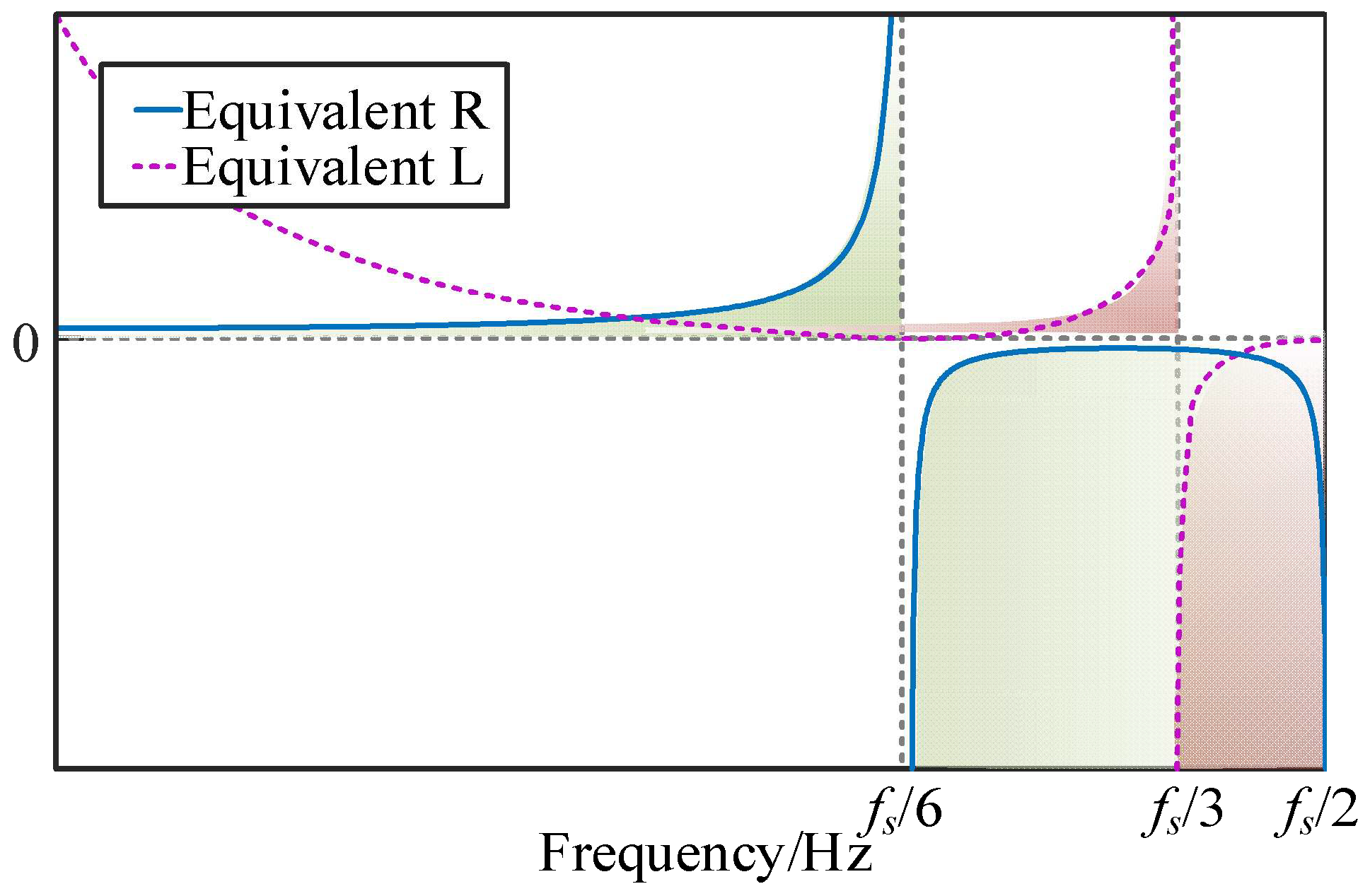
Influence of Switching Frequency
The delay resulting from digital control can influence the inverter’s output impedance. The magnitude of this delay is correlated with the switching frequency (fsw). Below is an analysis of how the switching frequency impacts the output impedance characteristics. Through block diagram transformation, it can be observed that the effect of the CCF-AD control strategy is equivalent to the passive damping method that involves paralleling a resistor across the terminals of the filter capacitor, as illustrated in Figure 9.
The delay introduced by digital control causes the equivalent resistance to become a frequency-dependent impedance, Zeqc, which can be expressed as:
Z eqc ( s ) = Z L 1 ( s ) Z C ( s ) H K i 1 PWM G d ( s ) = L 1 C H K i 1 PWM e 1.5 s T s
Based on the expressions for the equivalent resistance and equivalent reactance, their frequency characteristic curves are plotted. As shown in Figure 10, the equivalent resistance is no longer constant but varies with changes in the switching frequency and sampling frequency. It becomes negative damping at the frequency of fs/6. The equivalent reactance exhibits capacitive behavior at the frequency of fs/3. When the grid impedance varies over a wide range, the system’s resonant frequency shifts.
As the frequency approaches fs/6, the system becomes unstable. To reduce the effects of digital control delay, optimizing the delay is essential to improve system stability.
In summary, to ensure the stability of the inverter itself and its interaction stability under a strong grid, the control parameters for the inverter adopting capacitor current feedback control are selected as follows: Kp = 0.25, Kr = 10, and fsw = 5 kHz.

3. Stability Mechanism Analysis

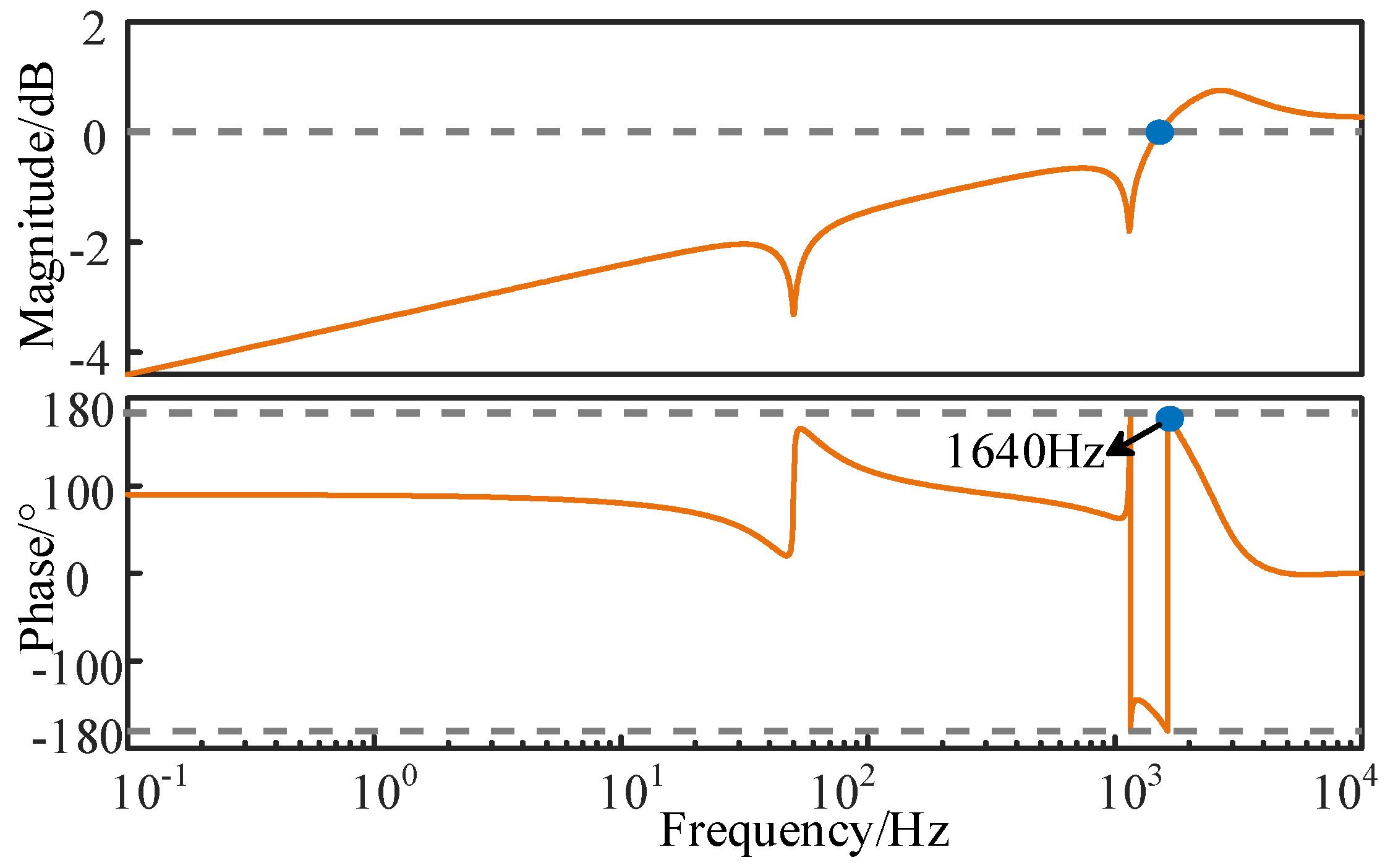
3.1. Stability Analysis of a Single Inverter

The fluctuations in grid impedance under weak grid circumstances can influence the stability of the system’s interaction. Figure 2, Figure 3, Figure 4, Figure 5, Figure 6, Figure 7, Figure 8, Figure 9, Figure 10 and Figure 11 illustrate the Nyquist curves of the equivalent loop gain of the system under different grid impedances. As the grid impedance changes from Lg = 100 mH to Lg = 700 mH, the Nyquist curve of the equivalent loop gain of the grid-connected system shifts from being far away from the (−1, j0) point to asymptotically encircling and then completely encircling the (−1, j0) point. As grid impedance increases, the grid becomes weaker, and the system’s stability deteriorates. When Lg = 400 mH, the system approaches critical stability.
When the grid impedance Lg is 700 mH, the loop gain Zg(s)/Zinv(s) of the system does not satisfy the Nyquist criterion. Figure 12 illustrates the magnitude–frequency characteristic curve, where the zero-crossing point—indicating the interaction between the inverter and grid impedances—occurs at the crossover frequency of 1650 Hz. At this frequency, the phase exceeds 180°, violating the Nyquist criterion and rendering the system unstable. In other words, the resonant frequency is 1650 Hz.

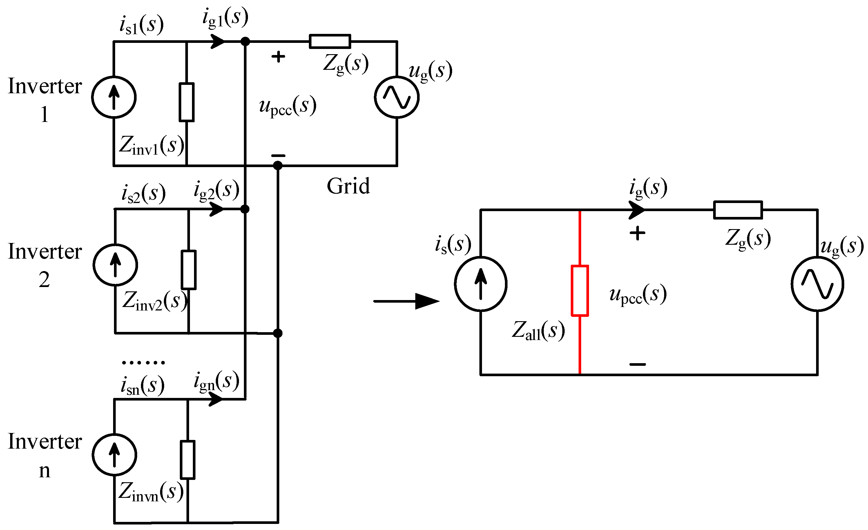
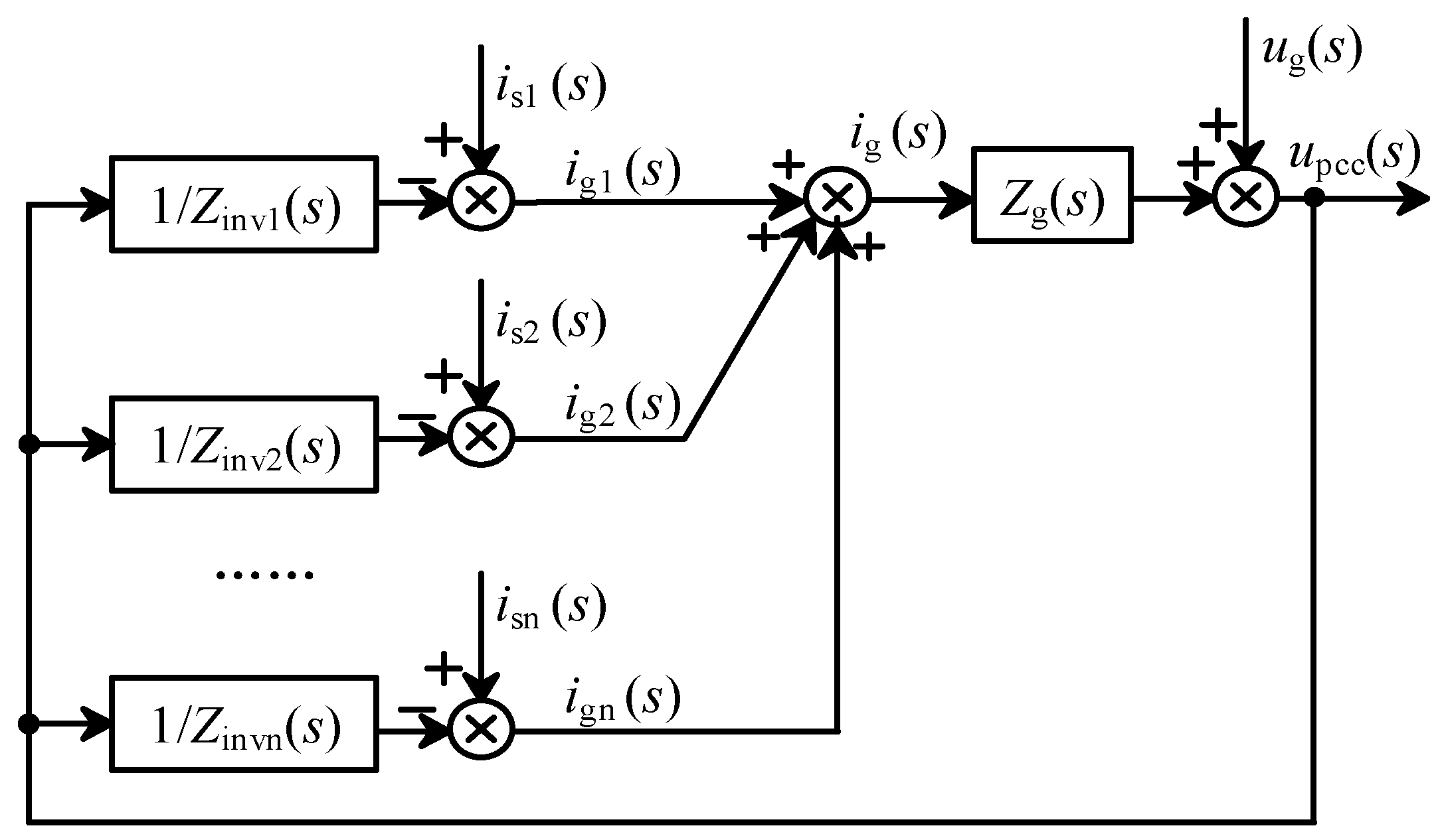
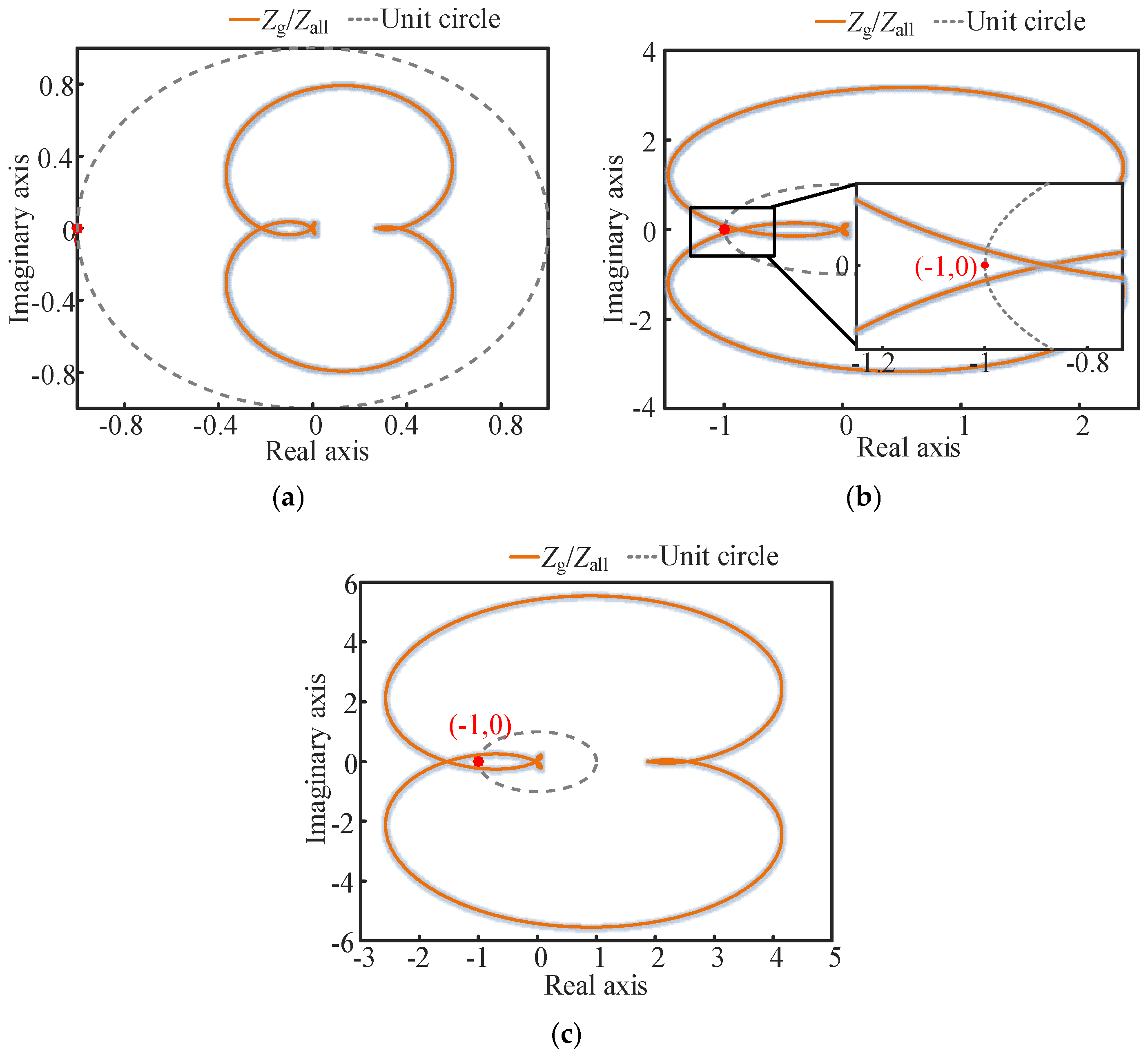
3.2. Stability Analysis of Multiple Inverters

When several inverters are connected to the grid at the same time, each can be represented at the Point of Common Coupling (PCC) by a Norton equivalent circuit, which consists of a current source isn(s) in parallel with an impedance Zinvn(s). The corresponding equivalent circuit is shown in Figure 13.
Zall(s) represents the total parallel impedance at the port. According to the superposition theorem, the voltage expression at the Point of Common Coupling (PCC) can be derived as follows:
u pcc ( s ) = Z all ( s ) Z g ( s ) Z all ( s ) + Z g ( s ) m = 1 n i sm ( s ) + Z all ( s ) Z all ( s ) + Z g ( s ) u g ( s ) = 1 1 + Z g ( s ) Z all ( s ) m = 1 n i sm ( s ) Z g ( s ) + u g ( s )
The mathematical model is derived from the equivalent circuit diagram of multiple inverters connected to the grid, as shown in Figure 14.
The expressions for the grid-connected current igm(s) of each inverter and the total grid-connected current ig(s) at the Point of Common Coupling (PCC) are given by:
i gm ( s ) = i sm ( s ) u pcc ( s ) Z invm ( s ) m = 1 , 2 , , n
i g ( s ) = u pcc ( s ) u g ( s ) Z g ( s )
Similar to the analysis of a single inverter connected to the grid as mentioned above, the stability conditions for multiple inverters connected to the grid are as follows:
  • Under a strong grid condition, each inverter ensures its own stability.
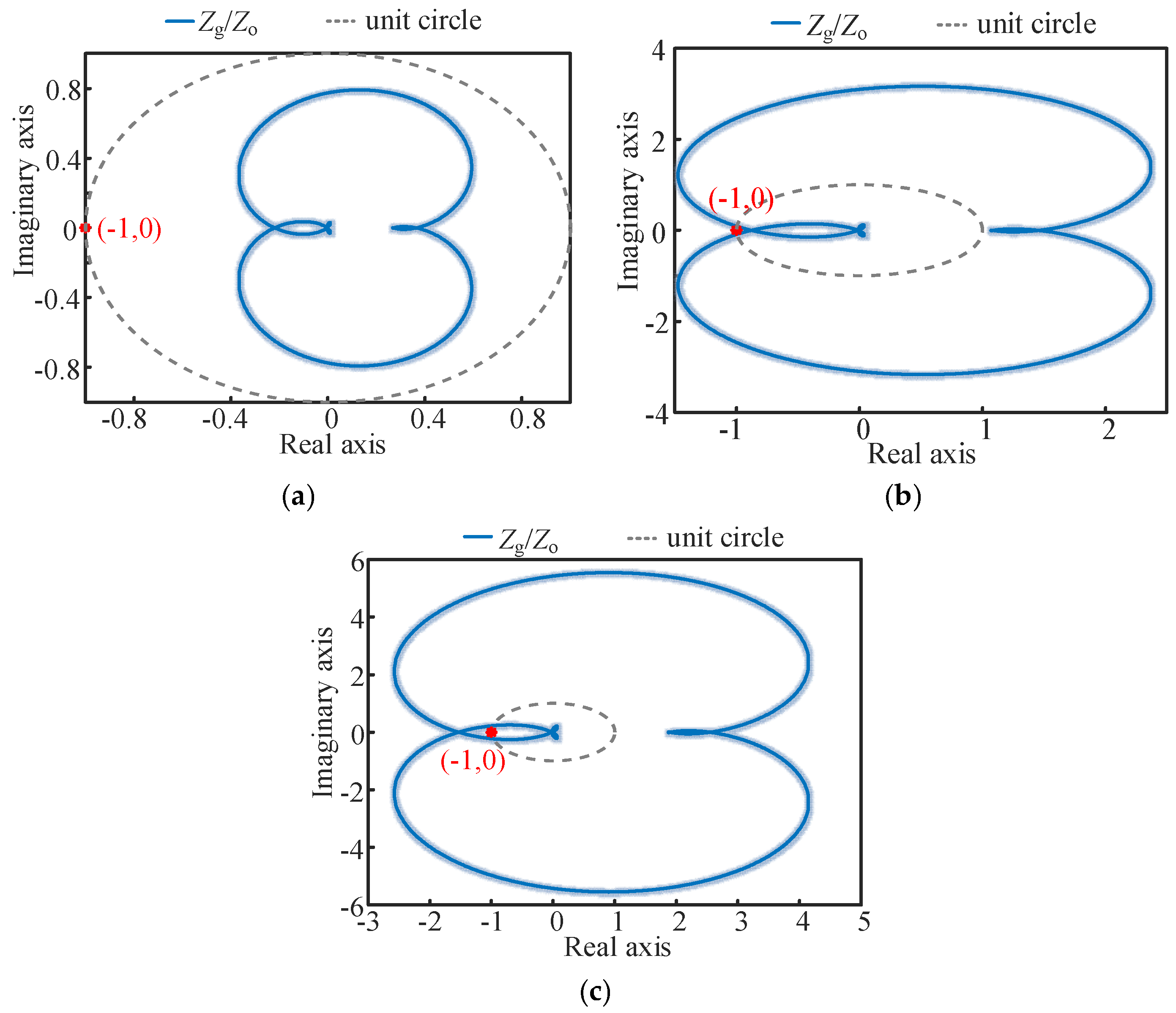
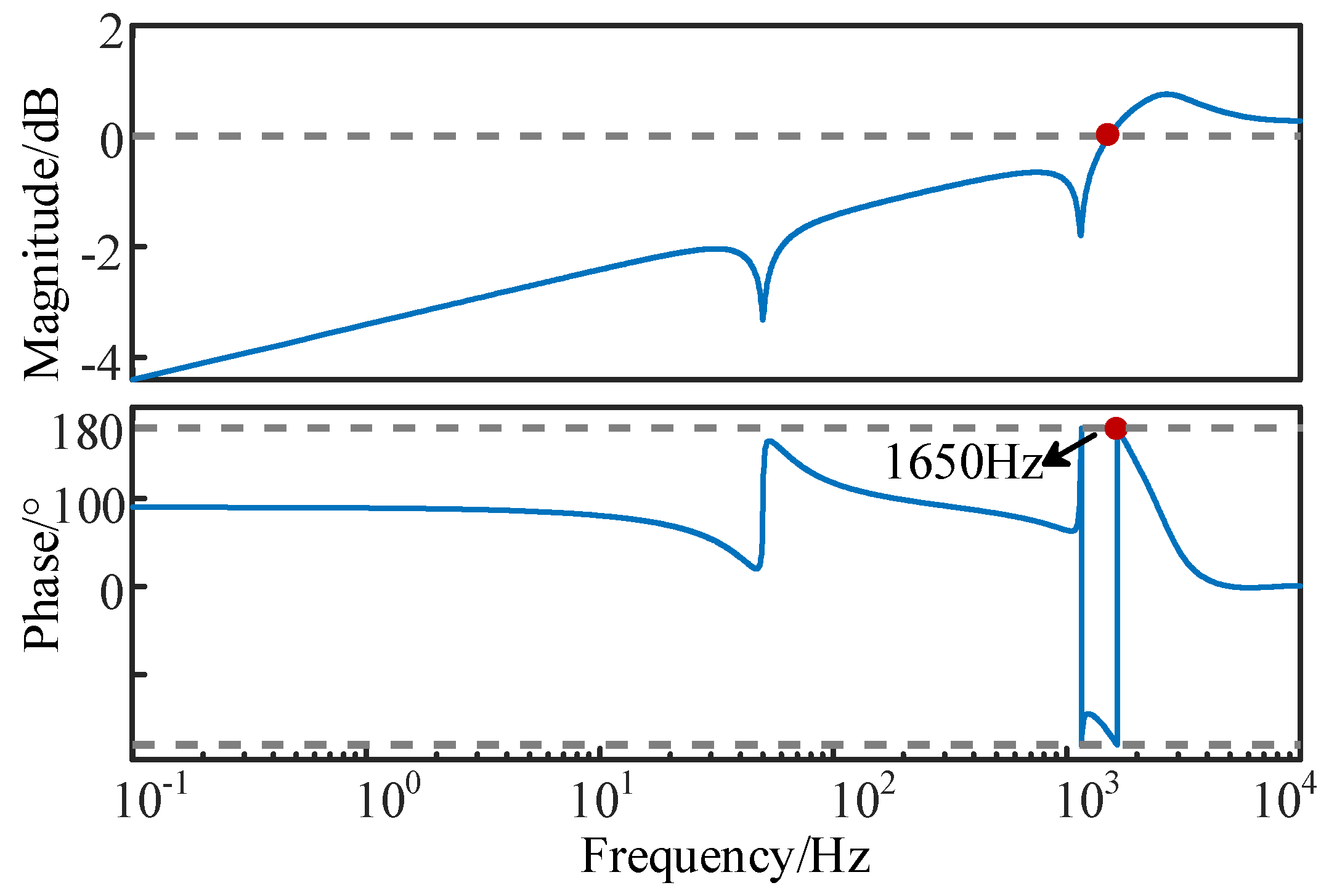
  • The equivalent loop gain Zg(s)/Zall(s) for multiple inverters connected to the grid meets the Nyquist criterion. The magnitude–frequency characteristic curve of the equivalent parallel impedance Zall(s) at the port does not intersect with that of the grid impedance. If they do intersect, the phase at the crossover frequency fc must be positive, meaning that the phase margin is satisfied.
PM = 180 ° ( Z g ( 2 π f c ) Z all ( 2 π f c ) ) > 0
A verification analysis is conducted based on two grid-connected inverters.
Figure 15 demonstrates the functioning of two inverters when linked to the grid, employing the traditional CCF-AD control strategy. Inverter 1 is a photovoltaic (PV) grid-connected inverter, while inverter 2 is an embedded energy storage grid-connected inverter. The circuit and control parameters of the inverters are listed in Table 3.
Figure 16 presents the Nyquist plots of the system’s equivalent loop gain for various grid impedances. As the grid impedance varies from Lg = 50 mH to Lg = 350 mH, the Nyquist curve of the equivalent loop gain of the grid-connected system shifts from being far away from the point (−1,j0) to gradually encircling and then completely encircling the point (−1,j0). As grid impedance increases, the grid weakens, and the system’s stability deteriorates. When Lg = 200 mH, the system approaches critical stability.
When the grid impedance Lg is 350 mH, the loop gain Zg(s)/Zall(s) of the multi-inverter system does not satisfy the Nyquist criterion. As shown in Figure 17, which depicts the magnitude–frequency characteristic curve, the point where the curve crosses zero—indicating the point where the inverter output impedance intersects with the grid impedance—occurs at a crossover frequency of 1640 Hz. At this frequency, the phase exceeds 180°, violating the Nyquist criterion and rendering the system unstable. This indicates that the resonant frequency is 1640 Hz.

4. Simulation Verifications

This section presents the construction of a simulation model for a single-phase embedded energy storage grid-connected inverter in MATLAB/Simulink 2023a, aimed at validating the inverter parameters and stability analysis using the CCF-AD control.

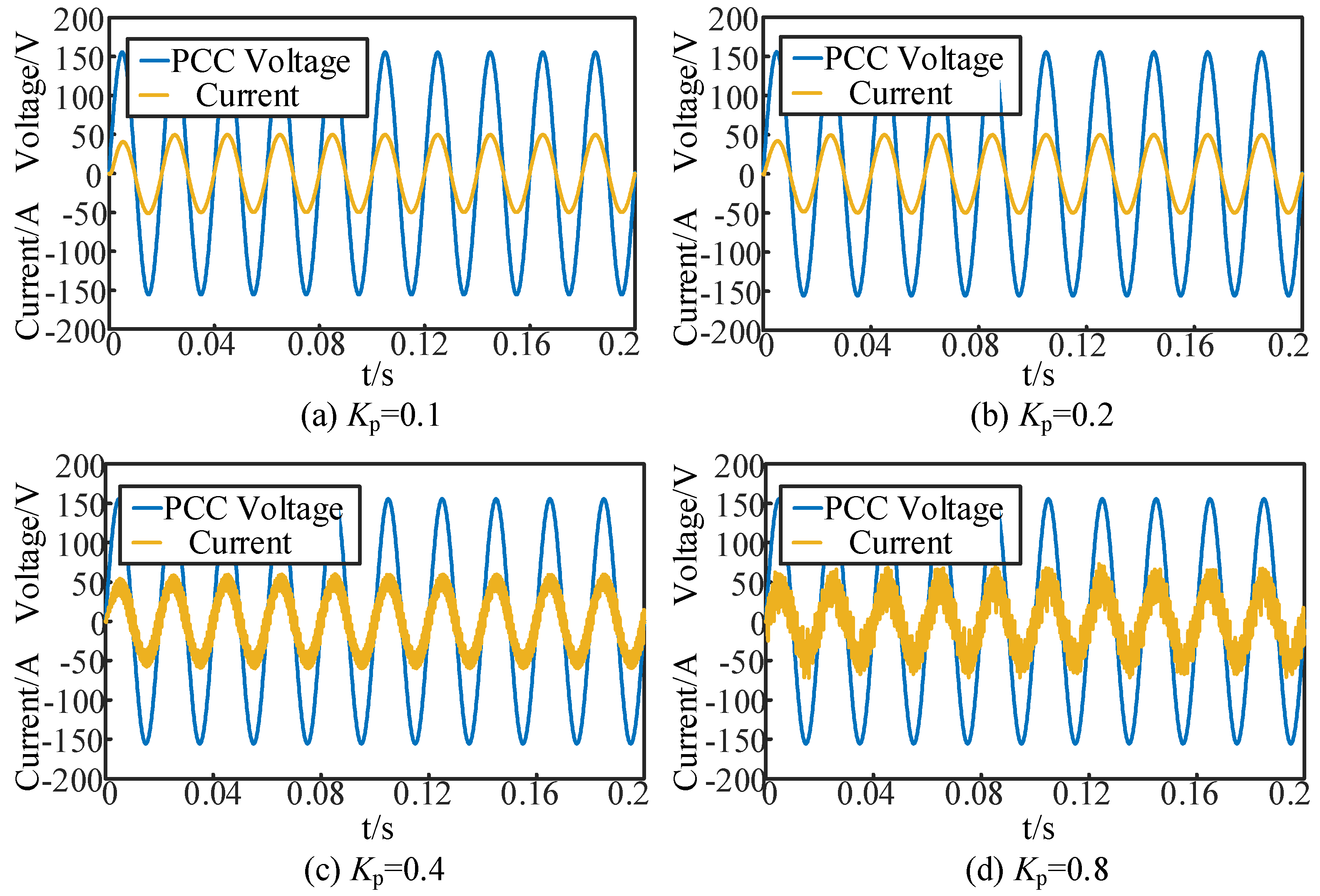
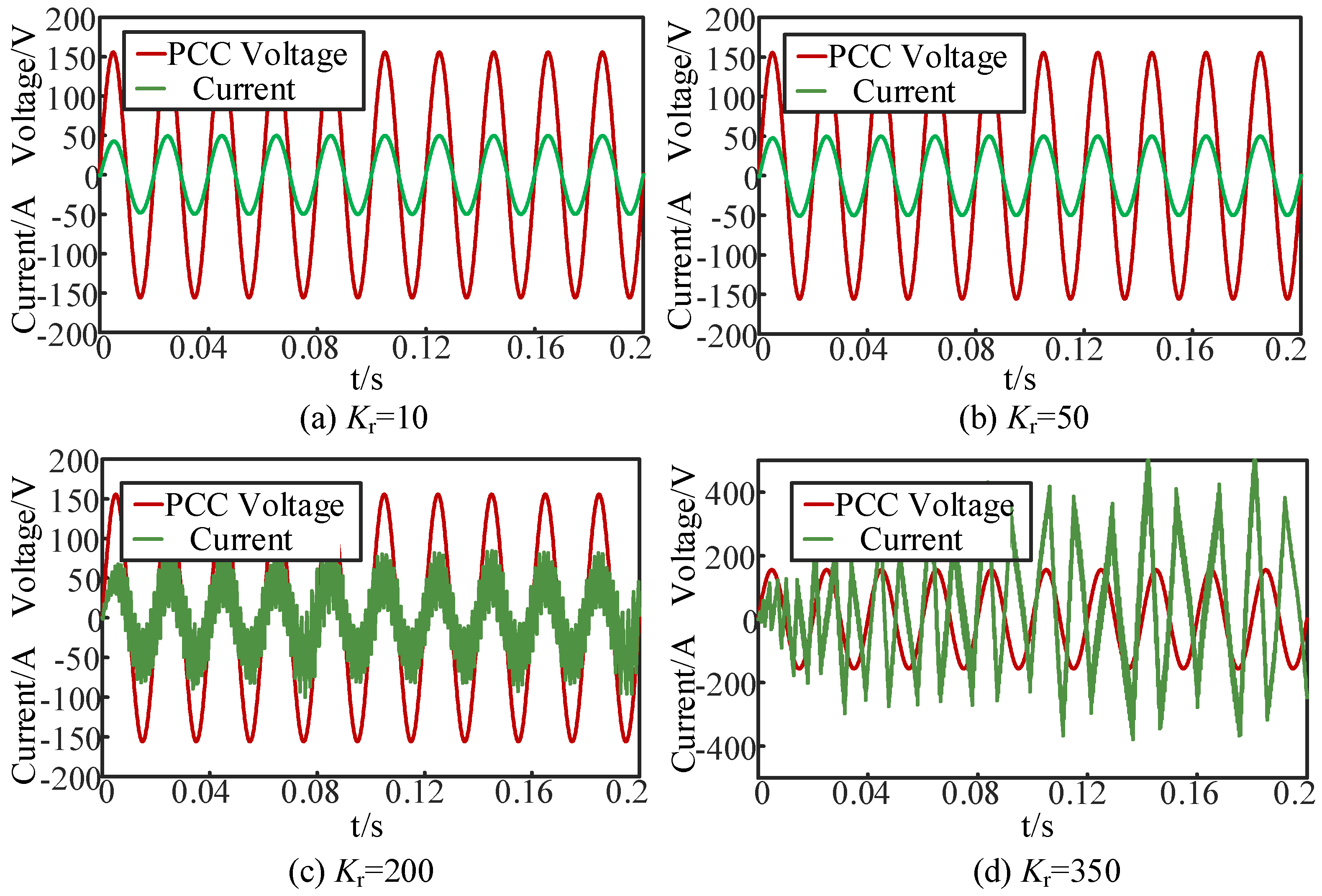
4.1. Verification of the Impact of Control Parameters

As the proportional coefficient Kp increases, the passivity region of the output impedance gradually decreases. However, when Kp reaches a certain value, the system resonates on its own and loses stability. Figure 18 presents four operating conditions with different proportional parameters, Kp. When Kp increases from 0.1 to 0.2, the current and voltage waveforms remain stable. As Kp continues to increase to 0.4, the current waveform resonates, and the system becomes unstable. When Kp further increases to 0.8, the degree of resonance intensifies. The simulation results demonstrate that increasing Kp leads to a decline in system stability, which aligns with the theoretical findings. Similarly, when the proportional coefficient Kp is fixed and the resonance coefficient Kr increases, the passivity region of the output impedance gradually expands.
However, a notable phenomenon occurs when the resonance parameter Kr attains a specific boundary value. At this juncture, the passivity region of the output impedance begins to diminish, and the system, in an unexpected turn of events, starts to resonate autonomously. This self-induced resonance causes the system to lose its inherent stability, leading to potential operational disruptions. Figure 19 vividly illustrates four distinct operating conditions, each characterized by a different value of the resonance parameter Kr. As Kr progressively increases from an initial value of 10 up to 350, a clear transformation in the output current waveform can be observed. Initially stable, the waveform gradually becomes divergent, a clear indication of the system’s resonance and subsequent instability. The simulation results provide compelling evidence that as the resonance coefficient Kr continues to escalate, the overall stability of the system correspondingly diminishes. This empirical finding is in perfect harmony with the theoretical analysis, thereby reinforcing the validity of the theoretical framework and providing valuable insights into the system’s behavior under varying resonance conditions.

4.2. Verification of the Stability Analysis in Single Inverter Case

Figure 20 shows the simulation waveforms of current and voltage for a single-inverter grid-connected system at different grid impedances: Lg = 100 mH, Lg = 400 mH, and Lg = 700 mH. In the first two cases, as the grid impedance rises from 100 mH to 400 mH, the system remains stable. The grid current is in sync with the voltage at the Point of Common Coupling (PCC), and the Total Harmonic Distortion (THD) of the current is under 5%, satisfying the grid connection requirements. However, when the grid impedance reaches Lg = 700 mH, a resonance between the current and voltage occurs, leading to system instability. This observation aligns with the stability analysis discussed earlier.
Figure 21 shows the FFT analysis of the grid-connected current when the grid impedance is 700 mH. The analysis indicates that the dominant harmonic frequency of the current is 1650 Hz, which matches the findings from the equivalent impedance Bode plot in Figure 12. These simulation results confirm the accuracy of the established model.

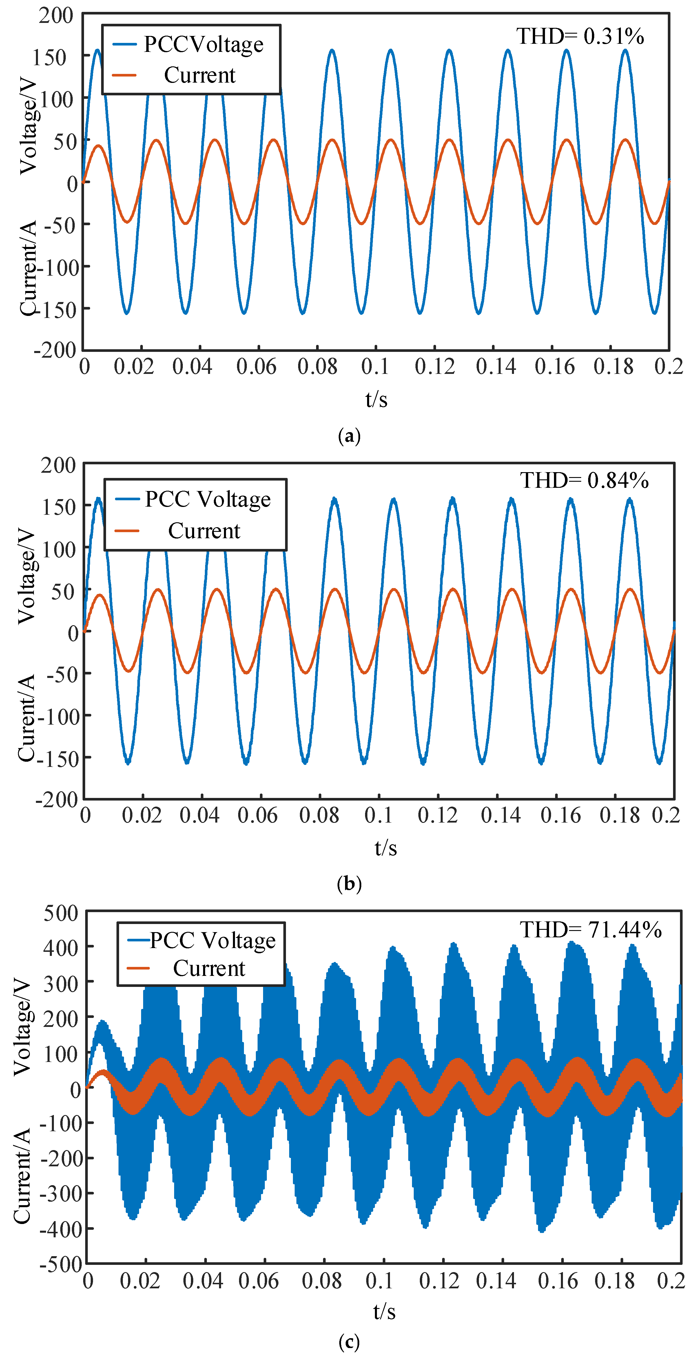
4.3. Verification of the Stability Analysis in Multiple Inverters Case

When wind–solar hybrid inverters 1 and 2 with embedded storages are put into operation, three operating conditions are set. For the first operating condition, with a grid impedance of Lg = 50 mH, the voltage and current at the Point of Common Coupling (PCC) of the grid-connected system are observed, as illustrated in Figure 22a. The analysis reveals that when the grid impedance is Lg = 50 mH, the Total Harmonic Distortion (THD) is 0.32%, and the current meets the grid connection standards. When the two inverters operate simultaneously in grid-connected mode, the system remains stable.
Maintaining the inverter parameters unchanged: when the grid impedance is increased to Lg = 200 mH, the voltage and current at the Point of Common Coupling (PCC) of the grid-connected system are observed, as shown in Figure 22b. The analysis indicates that with a grid impedance of Lg = 200 mH, the Total Harmonic Distortion (THD) is 0.74%, and the current meets the grid connection standards. When the two inverters operate simultaneously in the grid-connected mode, the system remains stable.
When the grid impedance is further increased to Lg = 350 mH, the voltage and current at the Point of Common Coupling (PCC) of the grid-connected system are observed, as depicted in Figure 22c. The analysis reveals that when the grid impedance is Lg = 350 mH, resonance occurs in both the current and voltage, leading to an unstable system, which is consistent with the theoretical analysis of Figure 23.

5. Conclusions

This study investigates the stability of grid-connected inverter systems incorporating embedded energy storage (EES). The research findings reveal the following:
(1)
The effect of the control parameters on a grid-connected inverter is demonstrated by a reduction in system stability as the proportional gain Kp increases. When Kp reaches a certain threshold, the system becomes unstable. Similarly, as the resonant coefficient Kr increases to a specific value, the system experiences resonance. To increase the stability of the inverter in practical applications, the values of Kp and Kr should be limited and, once the resonance occurs, decreasing the two parameters can be effective to suppress the oscillations.
(2)
The stability of the coupled system is affected by both the magnitude of grid impedance and the number of grid-connected inverters. As grid impedance increases, transitioning the system from a strong grid to a weak grid, system stability diminishes. Furthermore, even with a constant grid impedance, an increase in the number of grid-connected inverters also degrades system stability. Thus, the operation modes of the practical system should be paid attention to for the inverters connected to the grid.
However, because this study mainly focuses on voltage-sourced converters, an inverter based on current-sourced converters is not analyzed, but will be investigated in future.

Author Contributions

Investigation, J.Z.; methodology, G.Z.; validation, J.Z. and Y.J.; writing—original draft preparation, J.Z. and H.A.; writing—review and editing, H.A. and T.Z.; supervision, G.Z. All authors have read and agreed to the published version of the manuscript.

Funding

This work was supported by the State Grid Jiangsu Electric Power Co., Ltd. Technology Project under Grant J2024027. (Research on Multi-dimensional Stability Improvement Technology for Receiving-end Power Grids Based on Modular Energy Storage-Consumption Converter Technology).

Data Availability Statement

The raw data supporting the conclusions of this article will be made available by the authors on request.

Conflicts of Interest

The authors declare they are employees of State Grid Corporation of China (SGCC). The remaining authors declare that the research was conducted in the absence of any commercial or financial relationships that could be construed as a potential conflict of interest.

References

  1. Xie, X.; He, J.; Mao, H.; Li, H. New issues and classification of power system stability with high shares of renewables and power electronics. Proc. CSEE 2021, 41, 461–475. [Google Scholar]
  2. Jiang, Q.; Xu, R.; Li, B.; Chen, X.; Yin, Y.; Liu, T.; Blaabjerg, F. Impedance Model for Instability Analysis of LCC-HVDCs Considering Transformer Saturation. J. Mod. Power Syst. Clean Energy 2024, 12, 1309–1319. [Google Scholar]
  3. Li, Q.; Li, B.; Jiang, Q.; Liu, T.; Yue, Y.; Zhang, Y. A novel location method for interline power flow controllers based on entropy theory. Prot. Control Mod. Power Syst. 2024, 9, 70–81. [Google Scholar] [CrossRef]
  4. Ma, N.; Xie, X.; He, J.; Wang, H. Review of wide-band oscillation in renewable and power electronics highly integrated power systems. Proc. CSEE 2020, 40, 15. [Google Scholar]
  5. Bi, T.; Kong, Y.; Xiao, S.; Zhang, P.; Zhang, T. Review of sub-synchronous oscillation with large-scale wind power transmission. J. Electr. Power Sci. Technol. 2012, 27, 10–15. [Google Scholar]
  6. Dong, X.; Tian, X.; Zhang, Y.; Song, J. Practical SSR incidence and influencing factor analysis of DFIG-based series-compensated transmission system in Guyuan farms. High Volt. Eng. 2017, 43, 321–328. [Google Scholar]
  7. Feng, X.; Wu, J.; Cui, X. Sub-synchronous oscillation control strategy based on impedance identification for wind power grid-connected system in Guyuan area of China. Autom. Electr. Power Syst. 2023, 47, 200–207. [Google Scholar]
  8. Ma, J.; Shen, Y.; Du, Y.; Liu, H.; Wang, J. Overview on active damping technology of wind power integrated system adapting to broadband oscillation. J. Power Syst. Technol. 2021, 45, 1673–1686. [Google Scholar]
  9. Zhang, Y.; Yang, X.; Zhang, Z. High-Efficiency Broadband Electroacoustic Energy Conversion Using Non-Foster-Inspired Circuit and Adaptively Switched Capacitor. IEEE Trans. Ind. Electron. 2025, 1–12. [Google Scholar] [CrossRef]
  10. Yang, X.; Zhang, Z.; Xu, M.; Li, S.; Zhang, Y.; Zhu, X.-F.; Ouyang, X.; Alù, A. Digital non-Foster-inspired electronics for broadband impedance matching. Nat. Commun. 2024, 15, 4346. [Google Scholar] [CrossRef]
  11. Blaabjerg, F.; Chen, Z.; Kjaer, S.B. Power electronics as efficient interface in dispersed power generation systems. IEEE Trans. Power Electron. 2004, 19, 1184–1194. [Google Scholar] [CrossRef]
  12. Wang, X.; Blaabjerg, F.; Wu, W. Modeling and analysis of harmonic stability in an AC power-electronics-based power system. IEEE Trans. Power Electron. 2014, 29, 6421–6432. [Google Scholar] [CrossRef]
  13. Pogaku, N.; Prodanovic, M.; Green, T.C. Modeling, analysis and testing of autonomous operation of an inverter-based microgrid. IEEE Trans. Power Electron. 2007, 22, 613–625. [Google Scholar] [CrossRef]
  14. Sun, J. Impedance-based stability criterion for grid-connected inverters. IEEE Trans. Power Electron. 2011, 26, 3075–3078. [Google Scholar] [CrossRef]
  15. Wu, W.; Liu, Y.; He, Y.; Chung, H.S.H.; Liserre, M.; Blaabjerg, F. Damping methods for resonances caused by LCL-filter-based current-controlled grid-tied power inverters: An overview. IEEE Trans. Ind. Electron. 2017, 64, 7402–7413. [Google Scholar] [CrossRef]
  16. Awal, M.A.; Della Flora, L.; Husain, I. Observer based generalized active damping for voltage source converters with LCL filters. IEEE Trans. Power Electron. 2021, 37, 125–136. [Google Scholar] [CrossRef]
  17. Ruan, X. Control Technologies for LCL-Type Grid-Connected Inverters; Science Press: Beijing, China, 2015. [Google Scholar]
  18. Yang, S.; Lei, Q.; Peng, F.Z.; Qian, Z. A robust control scheme for grid-connected voltage-source inverters. IEEE Trans. Ind. Electron. 2010, 58, 202–212. [Google Scholar] [CrossRef]
  19. Liserre, M.; Dell’Aquila, A.; Blaabjerg, F. Genetic algorithm-based design of the active damping for an LCL-filter three-phase active rectifier. IEEE Trans. Power Electron. 2004, 19, 76–86. [Google Scholar] [CrossRef]
  20. Zhou, L.; Luo, A.; Chen, Y.; Zhou, X.; Li, M.; Kuang, H. Robust grid-current feedback active damping control method for LCL-type grid-connected inverters. Proc. CSEE 2016, 36, 2742–2752. [Google Scholar]
  21. Duan, X.; Li, P.; Zhao, F.; Chen, S.; Wang, J. Stability control of LCL-type grid-connected inverters based on full capacitor voltage feedforward in weak grids. High Volt. Eng. 2022, 48, 2140–2151. [Google Scholar]
  22. Peña-Alzola, R.; Liserre, M.; Blaabjerg, F.; Sebastián, R.; Dannehl, J.; Fuchs, F.W. Analysis of the passive damping losses in LCL-filter-based grid converters. IEEE Trans. Power Electron. 2012, 28, 2642–2646. [Google Scholar] [CrossRef]
  23. Wu, W.; He, Y.; Tang, T.; Blaabjerg, F. A new design method for the passive damped LCL and LLCL filter-based single-phase grid-tied inverter. IEEE Trans. Ind. Electron. 2012, 60, 4339–4350. [Google Scholar] [CrossRef]
  24. Xu, D.; Fei, W.; Yi, R. Passive damping of LCL, LLCL and LLCCL filters. Proc. CSEE 2015, 35, 4725–4735. [Google Scholar]
  25. Yin, J.; Xin, J.; Wu, X.; Tong, Y. Active damping control strategy for LCL filter based on band pass filter. Power Syst. Technol. 2013, 37, 2376–2382. [Google Scholar]
  26. Geng, Y.; Qi, Y.; Dong, W.; Deng, R. An active damping method with improved grid current feedback. Proc. CSEE 2018, 38, 5557–5567. [Google Scholar]
  27. Bao, C.; Ruan, X.; Wang, X.; Pan, D.; Li, W. Design of grid-connected inverters with LCL filter based on PI regulator and capacitor current feedback active damping. Zhongguo Dianji Gongcheng Xuebao Proc. Chin. Soc. Electr. Eng. 2012, 32, 25. [Google Scholar]
  28. Wang, A.; Ge, W.; Li, T.; Cui, D.; Li, M. Research on realization technology of active damping method with differential feedback of filter capacitance voltage for LCL filter based grid-connected inverters. J. Electr. Eng. 2023, 18, 126–132. [Google Scholar]
Figure 1. The topological structure.
Energies 18 03127 g001
Figure 2. The circuit and control diagram of a single-phase grid-connected inverter for BESS-MMC.
Energies 18 03127 g002
Figure 3. Bode plots of the two regulators.
Energies 18 03127 g003
Figure 4. Schematic diagram of unipolar double frequency modulation.
Energies 18 03127 g004
Figure 5. Block diagram of the inverter model using capacitor current feedback.
Energies 18 03127 g005
Figure 6. Simplified three-branch model.
Energies 18 03127 g006
Figure 7. Bode plot of the inverter’s output impedance for different Kp values. (a) Kp between 0.1 and 0.35; (b) Kp between 0.3 and 0.55.
Energies 18 03127 g007
Figure 8. Bode plot of the inverter’s output impedance for different Kr values. (a) Kr between 1 and 150; (b) Kr between 100 and 350.
Energies 18 03127 g008
Figure 9. Equivalent control block diagram for capacitor current feedback.
Energies 18 03127 g009
Figure 10. Frequency characteristic curves of equivalent resistance and reactance.
Energies 18 03127 g010
Figure 11. Stability analysis results of the grid-connected system under different grid impedance values. (a) Grid impedance Lg = 100 mH; (b) grid impedance Lg = 400 mH; (c) grid impedance Lg = 700 mH.
Energies 18 03127 g011
Figure 12. Bode plot of the equivalent loop gain of the system when the grid impedance Lg is 700 mH.
Energies 18 03127 g012
Figure 13. Equivalent circuit diagram for multiple inverters.
Energies 18 03127 g013
Figure 14. Block diagram of the mathematical model for multiple inverters.
Energies 18 03127 g014
Figure 15. Circuit diagram of two inverters.
Energies 18 03127 g015
Figure 16. Stability analysis results of the multi-grid-connected inverters. (a) Grid impedance Lg = 50 mH; (b) grid impedance Lg = 200 mH; (c) grid impedance Lg = 350 mH.
Energies 18 03127 g016
Figure 17. Bode plot of the equivalent loop gain of the system when the grid impedance Lg is 350 mH.
Energies 18 03127 g017
Figure 18. Simulation results with different proportional parameters.
Energies 18 03127 g018
Figure 19. Simulation results with different resonance parameters.
Energies 18 03127 g019
Figure 20. Simulation results of with different grid impedance values. (a) Grid impedance Lg = 100 mH; (b) grid impedance Lg = 400 mH; (c) grid impedance Lg = 700 mH.
Energies 18 03127 g020
Figure 21. FFT analysis spectrum diagram of grid-connected current in single inverter case.
Energies 18 03127 g021
Figure 22. Simulation results of with different grid impedance values in multiple inverters case. (a) Grid impedance Lg = 50 mH; (b) grid impedance Lg = 200 mH; (c) grid impedance Lg = 350 mH.
Energies 18 03127 g022
Figure 23. FFT analysis spectrum diagram of grid-connected current in multiple inverters case.
Energies 18 03127 g023
Table 1. A comparison of different methods.
MethodsDescription
Resonance Peak Damping MethodsPassive DampingAchieved by series or parallel resistors in the circuit
Simple and effective, but introduces losses
Active DampingNo additional losses introduced, more flexible damping implementation
Analysis of Passive Damping MethodsRd Damping MethodDampens resonance but affects gain characteristics in the high-frequency range, reducing high-frequency harmonic attenuation
Rd-Cd Hybrid Resistor–Capacitor Passive Damping MethodDampens resonance without affecting high-frequency harmonic attenuation by adding capacitance
Analysis of Active Damping MethodsMethods Without Additional SensorsAchieved through grid-connected current feedback or filter parameter estimation
Methods Requiring Additional SensorsFeedback voltage or other currents for virtual damping control
Most Widely Used MethodActive Damping Based on Capacitor Current Proportional FeedbackEquivalent to passive damping by paralleling a resistor across the capacitor
Provides virtual resistance for damping, easy to implement without introducing additional losses
Table 2. Key parameters of the inverter.
ParametersValue
Grid voltage (ug/V)110
DC-side voltage (Udc/V)300
Triangular carrier amplitude (Utri/V)1
Inverter-side inductance (L1/mH)2
Filter capacitor (C/μF)10
Grid-side inductance (L2/mH)400
Grid-connected current sampling coefficient (Hi2)0.15
Capacitor current feedback coefficient (Hi1)0.002
Table 3. Key parameters of the two grid-connected inverters.
ParametersValue
Grid voltage (ug/V)110
DC-side voltage (Udc/V)300
Rated capacity (S/VA)4000
Inverter-side inductance (L1/mH)2
Filter capacitor (C/μF)10
Grid-side inductance (L2/mH)400
Gi(s) proportionality coefficient (Kp)0.25
Gi(s) Resonance coefficient (Kr)10
Switching frequency (fsw/kHz)5
Sampling frequency (fs/kHz)10
Grid-connected current sampling coefficient (Hi2)0.15
Capacitor current feedback coefficient (Hi1)0.002
Disclaimer/Publisher’s Note: The statements, opinions and data contained in all publications are solely those of the individual author(s) and contributor(s) and not of MDPI and/or the editor(s). MDPI and/or the editor(s) disclaim responsibility for any injury to people or property resulting from any ideas, methods, instructions or products referred to in the content.

