Author Contributions
Conceptualization, A.U. and M.P.; methodology, A.U. and M.P.; software, A.U.; validation, A.U.; formal analysis, A.U.; investigation, A.U.; resources, A.U.; data curation, A.U.; writing—original draft preparation, A.U.; writing—review and editing, A.U. and M.P.; visualization, A.U.; supervision, M.P.; project administration, M.P.; funding acquisition, M.P. All authors have read and agreed to the published version of the manuscript.
Figure 1.
The flowchart of obtaining, analyzing, and scaling ISO-NE time-series data to an IEEE test system for regional load forecasting.
Figure 1.
The flowchart of obtaining, analyzing, and scaling ISO-NE time-series data to an IEEE test system for regional load forecasting.
Figure 2.
Hourly historical load profiles for CT and ME from 2017 to 2022.
Figure 2.
Hourly historical load profiles for CT and ME from 2017 to 2022.
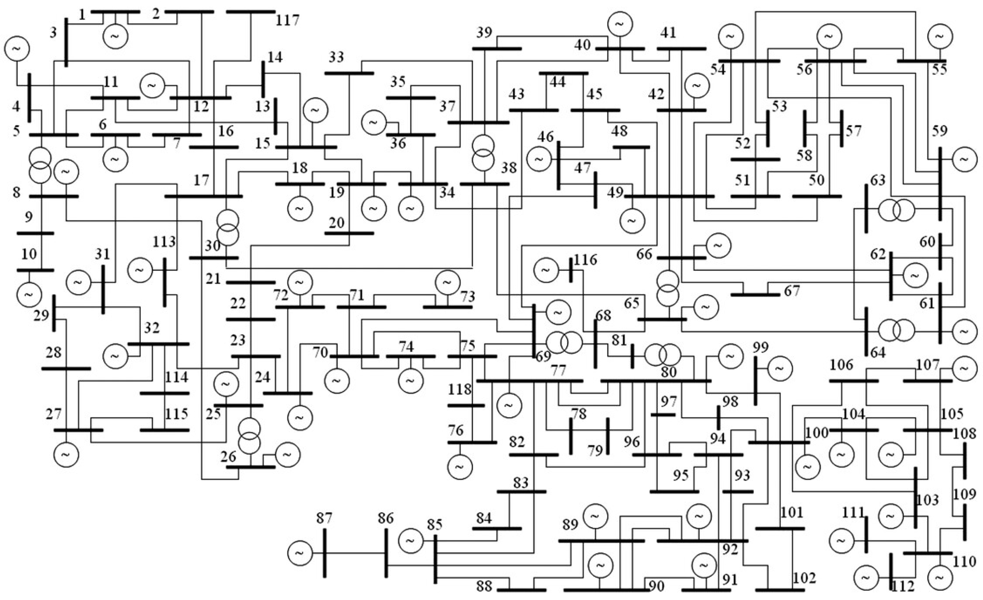
Figure 3.
IEEE 118-bus test system topology used for deep learning experiments. The buses are grouped into regions corresponding to U.S. states (CT, RI, NH, VT, ME) and subregions within Massachusetts (SEMA, NEMA, WCMA), explained in
Table 3 and
Table 4.
Figure 3.
IEEE 118-bus test system topology used for deep learning experiments. The buses are grouped into regions corresponding to U.S. states (CT, RI, NH, VT, ME) and subregions within Massachusetts (SEMA, NEMA, WCMA), explained in
Table 3 and
Table 4.
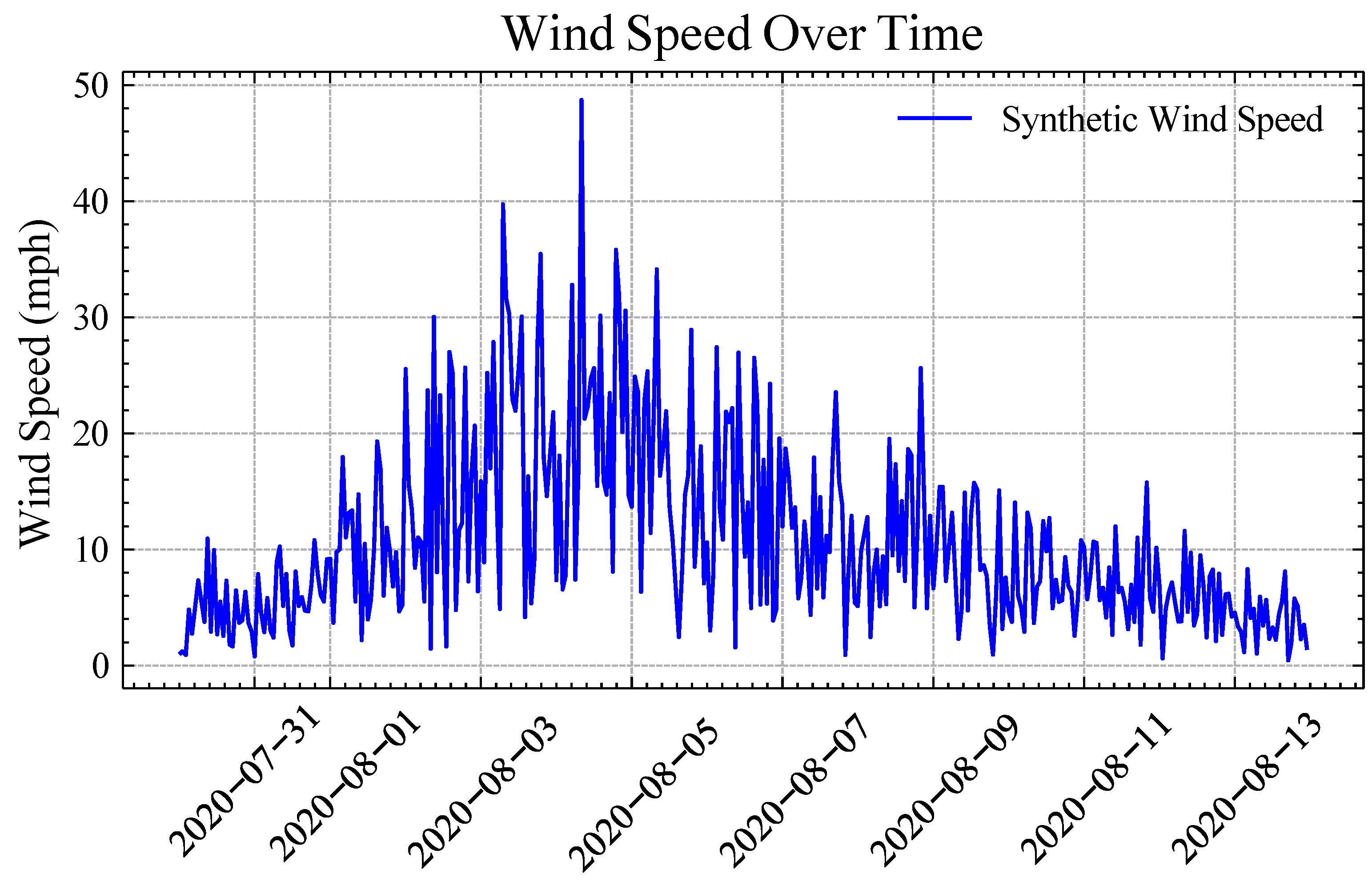
Figure 4.
Illustration of synthetic wind speed for hurricane Isaias.
Figure 4.
Illustration of synthetic wind speed for hurricane Isaias.
Figure 5.
Hurricane Isaias weather plots for illustrating atmospheric changes during 2020.
Figure 5.
Hurricane Isaias weather plots for illustrating atmospheric changes during 2020.
Figure 6.
Hurricane Isaias (2020) load behavior during normal and hurricane conditions.
Figure 6.
Hurricane Isaias (2020) load behavior during normal and hurricane conditions.
Figure 7.
RNN unit network structure.
Figure 7.
RNN unit network structure.
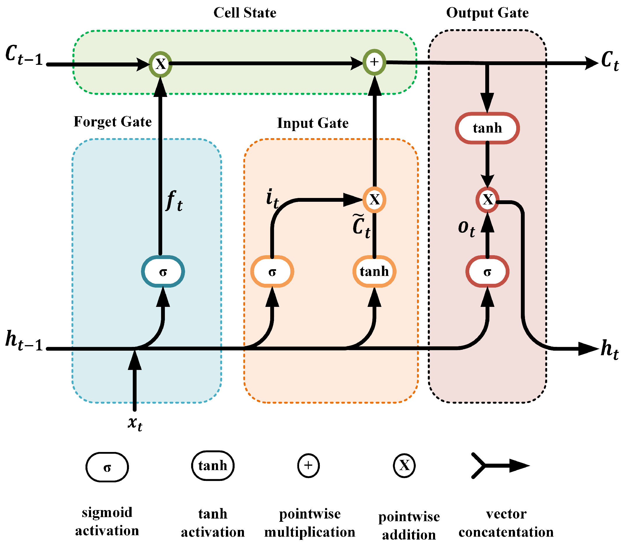
Figure 8.
LSTM unit network structure.
Figure 8.
LSTM unit network structure.
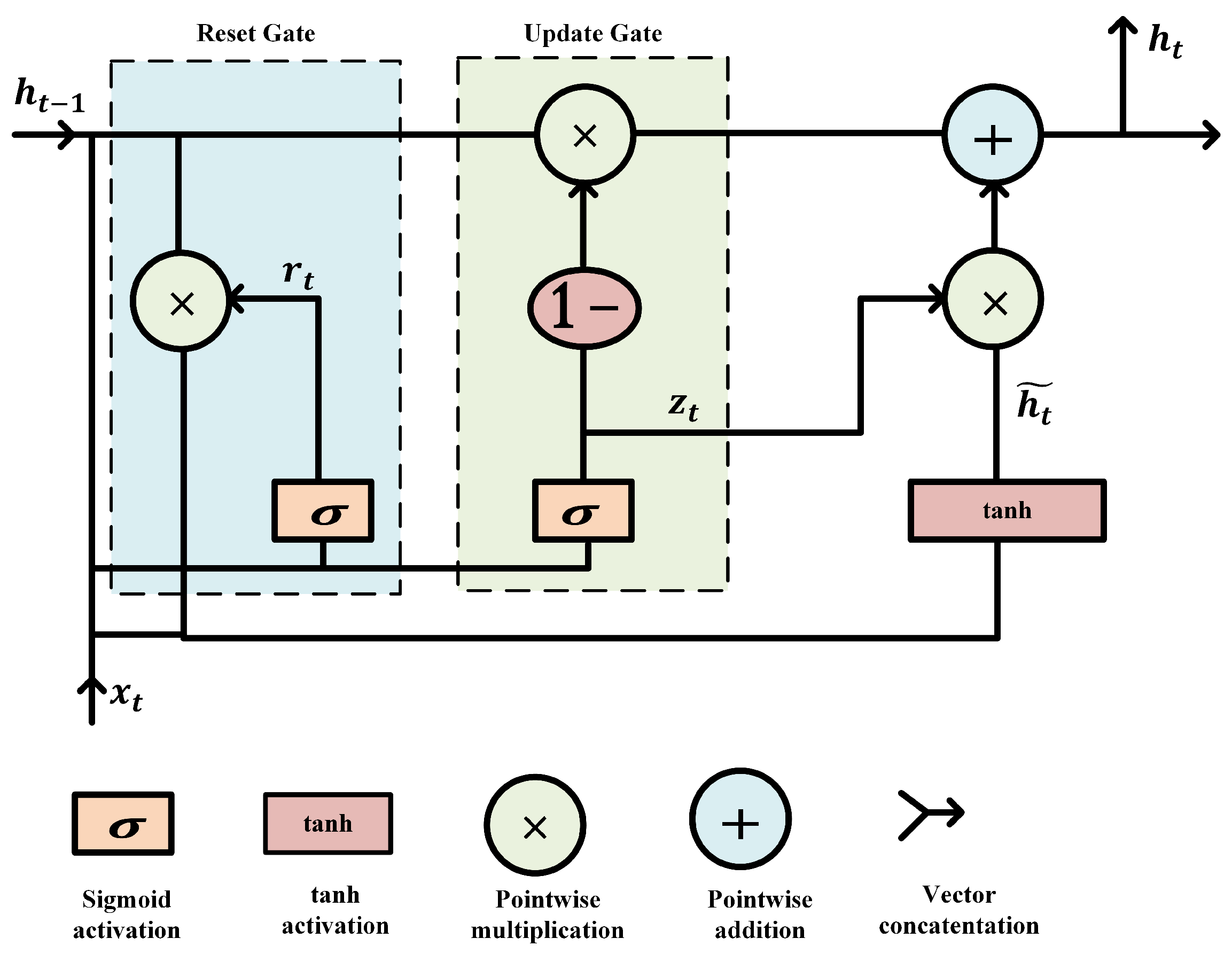
Figure 9.
GRU unit network structure.
Figure 9.
GRU unit network structure.
Figure 10.
General structure of a bidirectional recurrent network for BiRNN, BiLSTM, and BiGRU models.
Figure 10.
General structure of a bidirectional recurrent network for BiRNN, BiLSTM, and BiGRU models.
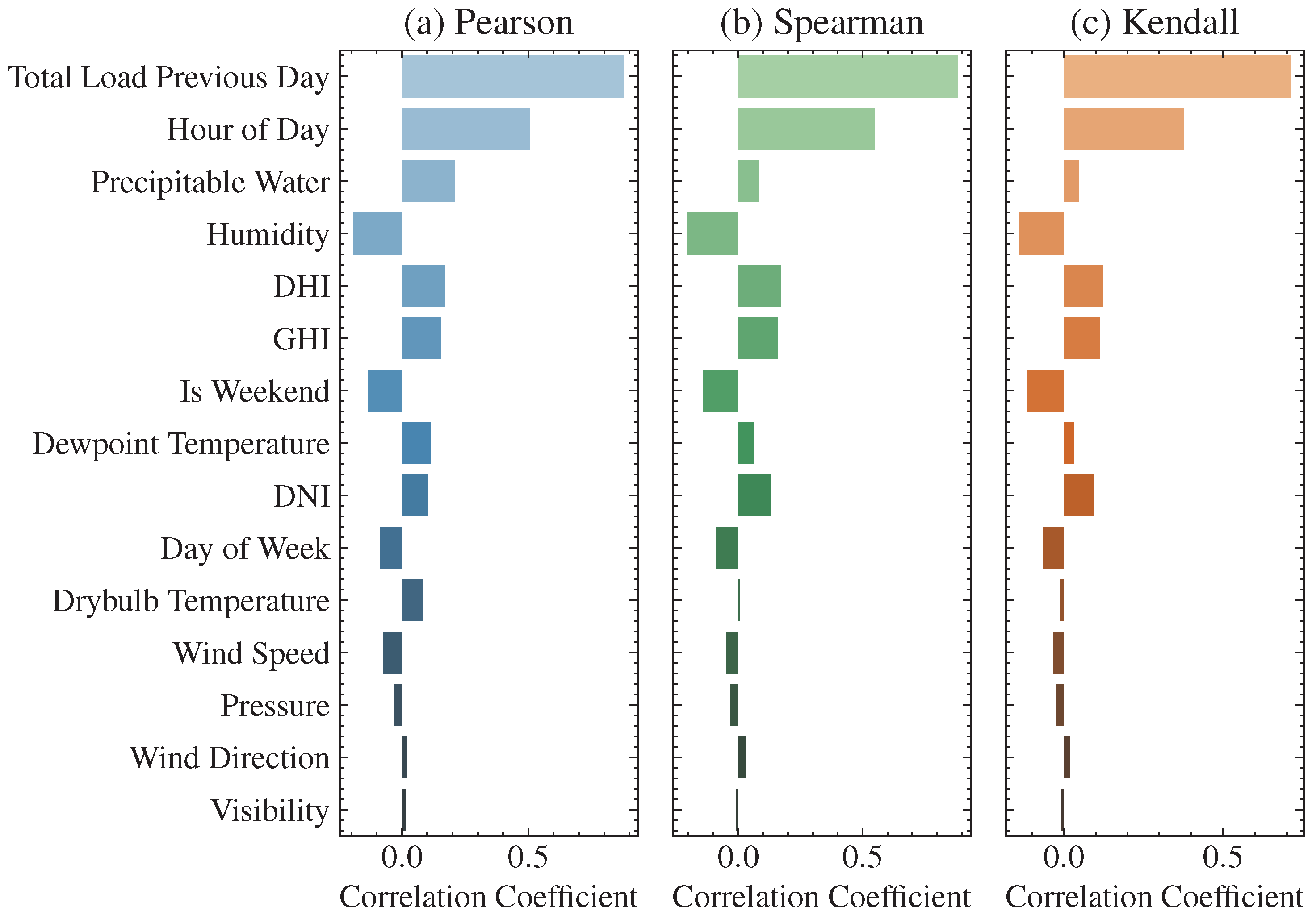
Figure 11.
Correlation coefficients between one of the system buses and exogenous variables using (a) Pearson, (b) Spearman, and (c) Kendall methods. Different colors are used to show each correlation type, such as blue for Pearson, green for Spearman, and orange for Kendall.
Figure 11.
Correlation coefficients between one of the system buses and exogenous variables using (a) Pearson, (b) Spearman, and (c) Kendall methods. Different colors are used to show each correlation type, such as blue for Pearson, green for Spearman, and orange for Kendall.
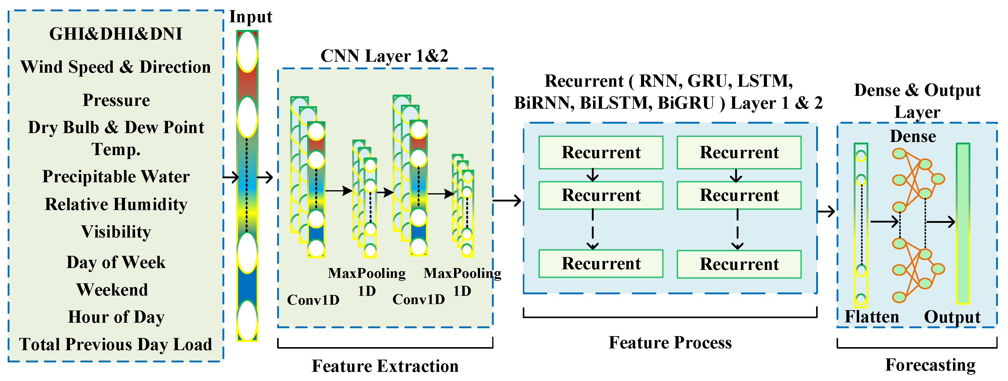
Figure 12.
Architecture of the combined deep learning model for short-term load forecasting. The model integrates CNN for feature extraction and RNN-based stacked layers (RNN, GRU, LSTM, BiRNN, BiGRU, or BiLSTM) for temporal modeling and process, using weather, calendar, and historical load data as inputs. A dense output layer provides the hour-ahead forecast.
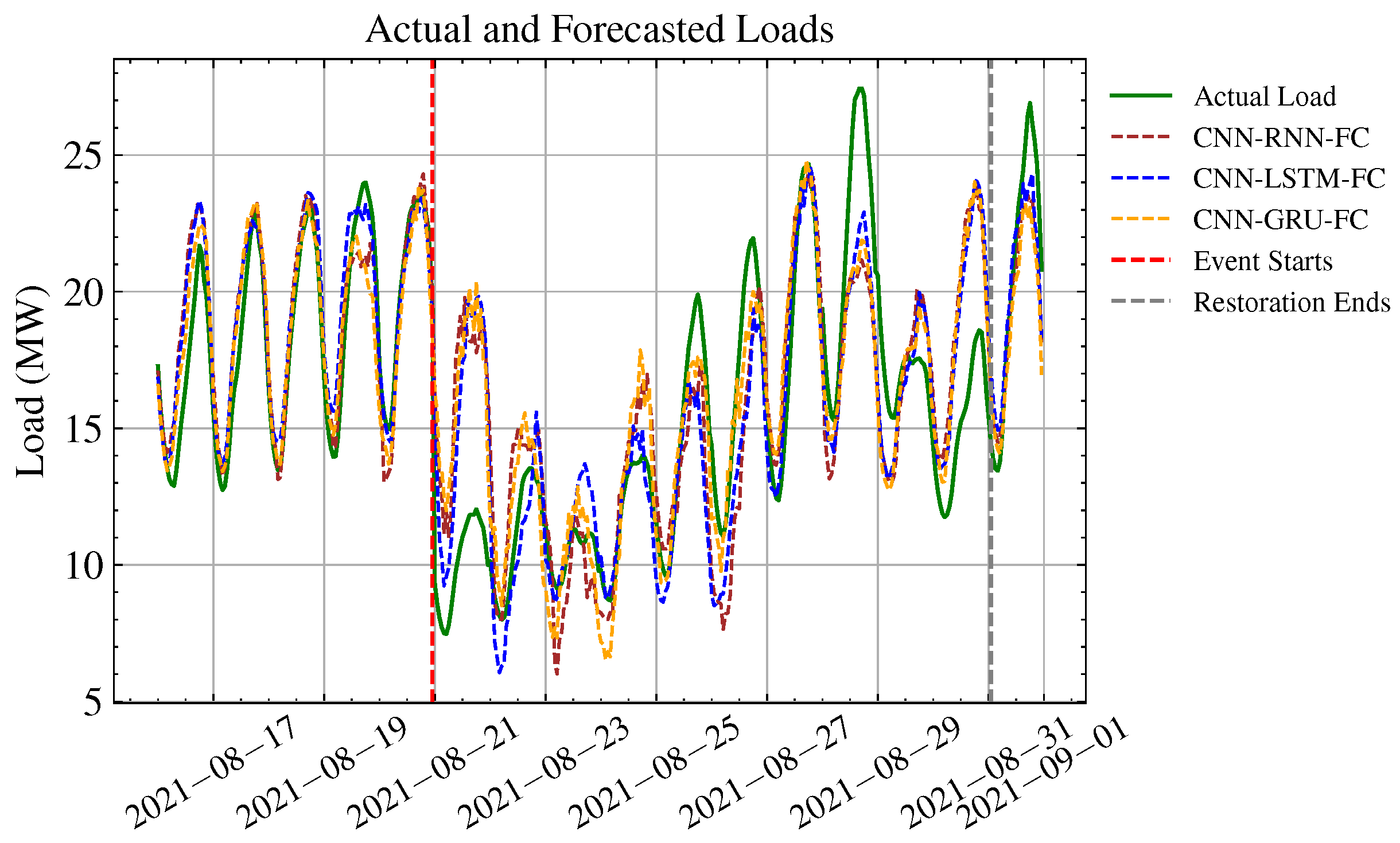
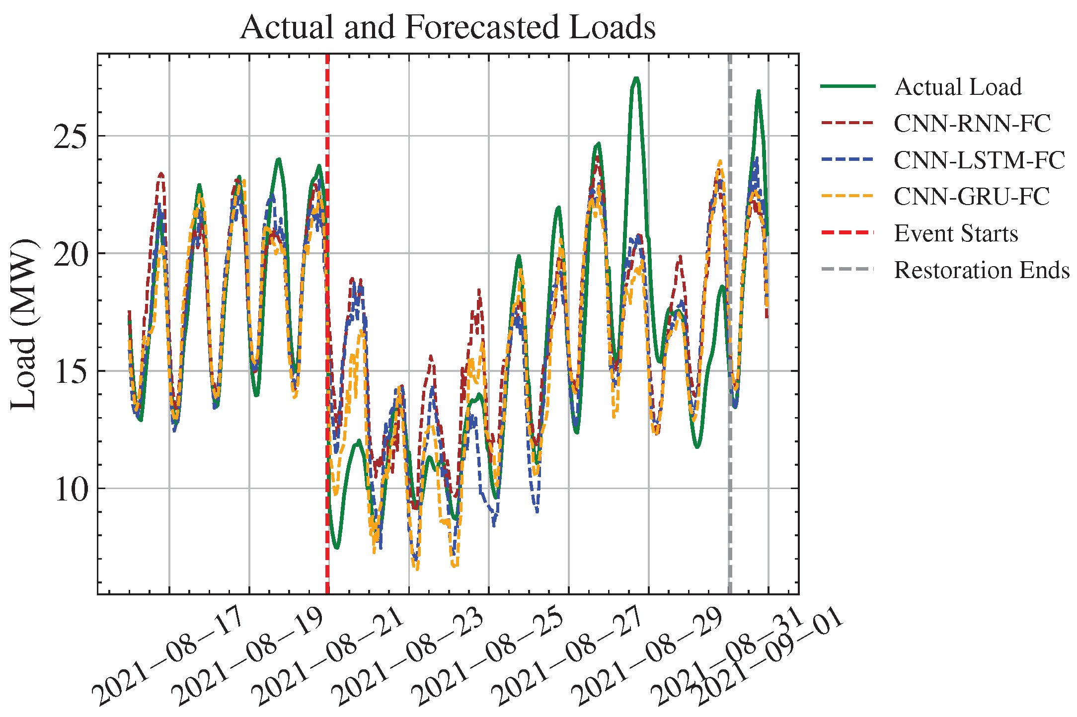
Figure 13.
Forecast and actual load for Hurricane Henri.
Figure 13.
Forecast and actual load for Hurricane Henri.
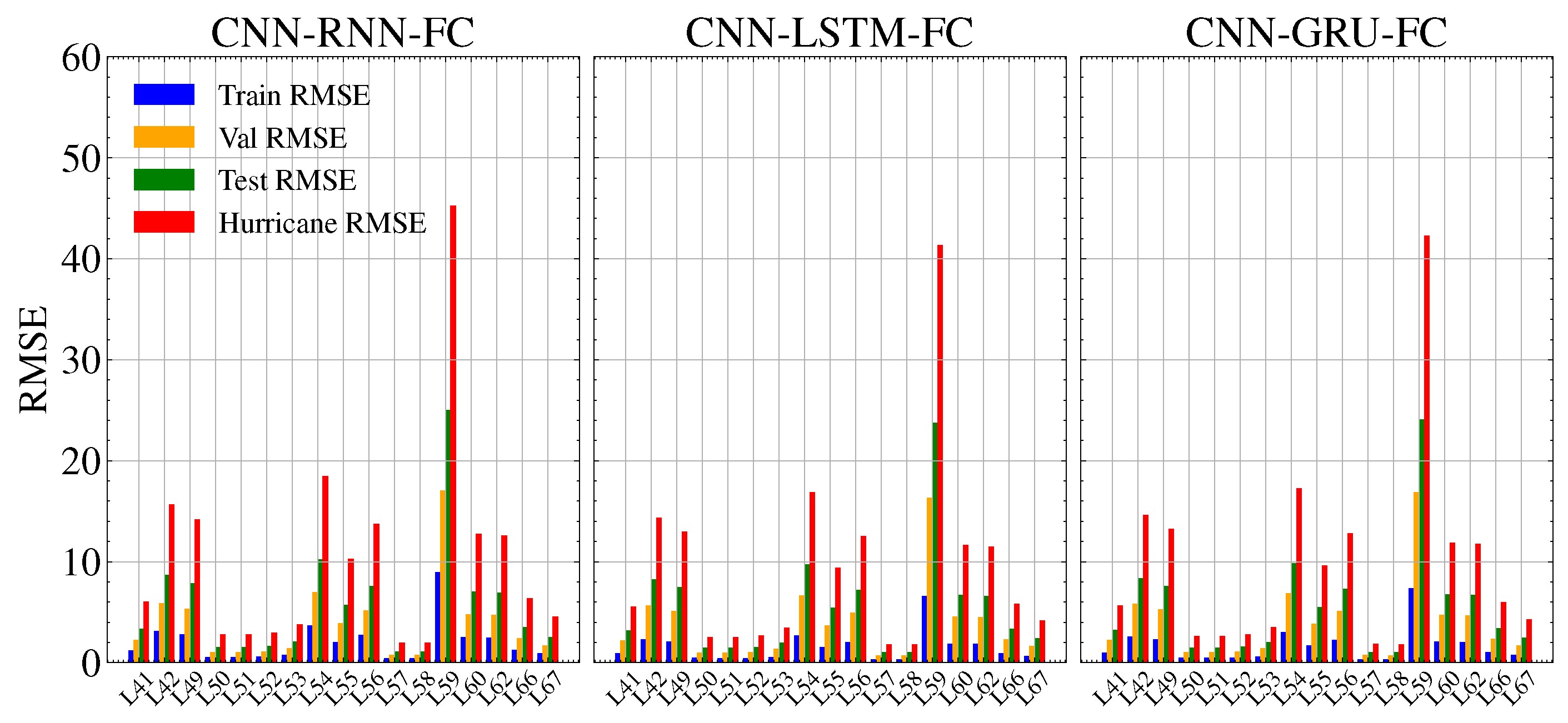
Figure 14.
Train, validation, test and hurricane dataset errors for each bus.
Figure 14.
Train, validation, test and hurricane dataset errors for each bus.
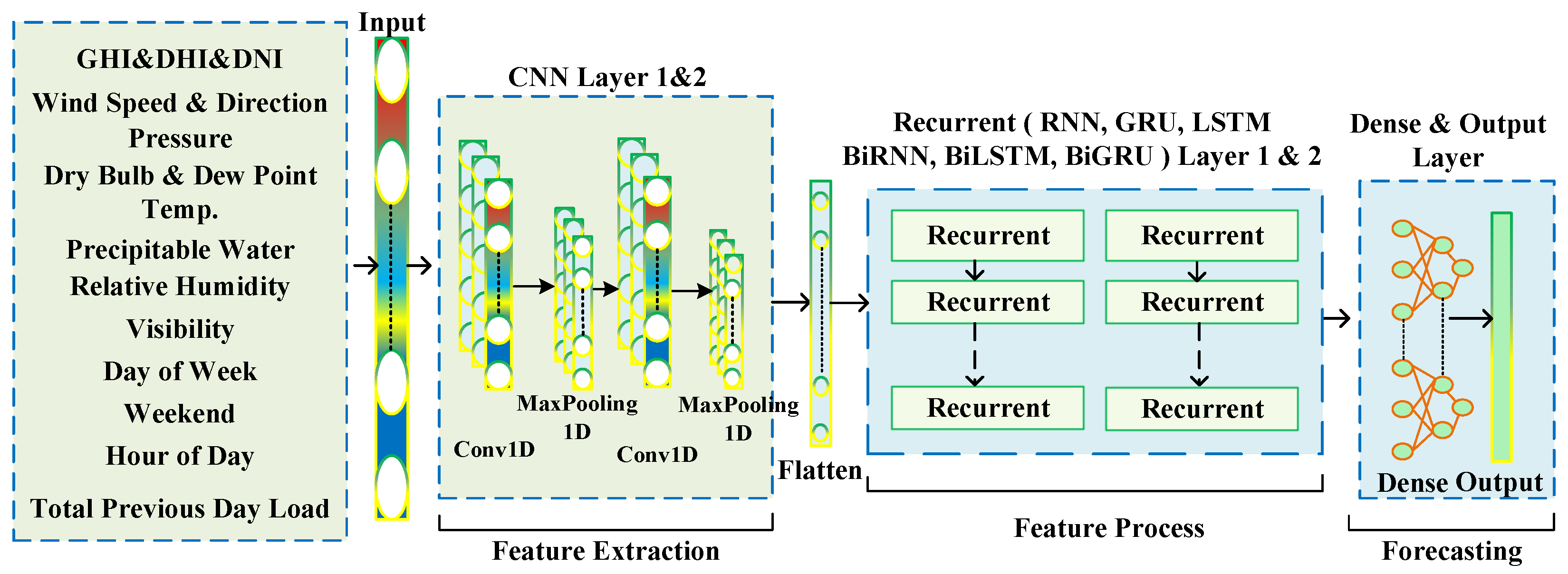
Figure 15.
Architecture of the hybrid deep learning model. The model combines CNN for feature extraction with RNN-based stacked layers (RNN, GRU, LSTM, BiRNN, BiGRU, or BiLSTM) for temporal modeling and processing, using weather, calendar, and historical load data as inputs. A dense output layer provides the hour-ahead forecast.
Figure 16.
Forecast and actual load for hurricane Henri.
Figure 16.
Forecast and actual load for hurricane Henri.
Figure 17.
Train, validation, test, and hurricane dataset errors for each bus.
Figure 17.
Train, validation, test, and hurricane dataset errors for each bus.
Table 1.
Summary of related works on hybrid and bidirectional deep learning models for load forecasting under normal and extreme weather conditions.
Table 1.
Summary of related works on hybrid and bidirectional deep learning models for load forecasting under normal and extreme weather conditions.
| Model Type | Dataset | Features | Horizon | Main Findings |
|---|
| BiGRU/ViT | Australian wildfire data | Calendar, temperature, fire weather index | Short-term (30–60 min) | BiGRU and ViT improved forecast accuracy. ViT had better trend performance. BiGRU resulted in the most outstanding results [36]. |
| FATCN-LF-FAGSNP | European national grid data | Weather, seasonal, extreme weather indicators | Short-term (60 min) | Hybrid model obtained high accuracy by using membrane computing and multi-level decomposition [39]. |
| CNN-LSTM | ISO New England (ISO-NE) load | Weather, calendar | Short-term (60 min) | Compared combined DL architectures. CNN-LSTM performed best using exogenous features [30]. |
| CNN-Informer | China (three-city load) | Load sequences | Short-term (60 min) | Transfer learning and hybrid ensemble improved accuracy on small-sample forecasting [40]. |
| SARIMAX-LSTM | Korea daily peak load | Weather, calendar | Day ahead (24 h) | Hybrid DL model outperformed standalone ML/DL methods [35]. |
| TCN-BiGRU (Fusion) | Arizona State Univ. (USA) campus load | Electric, cooling, heating, weather | Short-term (60 min) | Adaptive hybrid decomposition and multi-model prediction improved forecasting performance [38]. |
| CNN-BiLSTM + XGBoost | China one-city load | Weather, calendar | Short-term (15 min) | Adaptive clustering and stacked model improved generalization and reduced forecasting error on selected days [37]. |
Table 2.
Overall IEEE 118 test systems.
Table 2.
Overall IEEE 118 test systems.
| Test System | No. of Buses | No. of Gens | No. of Loads | LOAD (MW) | LOAD (MVAR) |
|---|
| IEEE 118 | 118 | 19 | 91 | 4242 | 1438 |
Table 3.
Region-bus group assignment for CT, RI, NH, and VT.
Table 3.
Region-bus group assignment for CT, RI, NH, and VT.
| | CT | RI | NH | VT |
|---|
| IEEE118 | 41–42, 49–52, 53–59, 60–64, 66–67 | 33–36, 37, 39–40, 43–48 | 89–92, 93–97, 98–102 | 82–85, 86–88 |
Table 4.
Region-bus group assignment for SEMA, NEMA, WCMA, and ME.
Table 4.
Region-bus group assignment for SEMA, NEMA, WCMA, and ME.
| | SEMA | NEMA | WCMA | ME |
|---|
| IEEE118 | 1–6, 7, 11–20, 117 | 8–10, 21–32, 70–72, 113–115 | 38, 65, 68–69, 73–81, 116, 118 | 103–108, 109–112 |
Table 5.
Hyperparameter search space for CNN-RNN-FC, CNN-GRU-FC, and CNN-LSTM-FC models.
Table 5.
Hyperparameter search space for CNN-RNN-FC, CNN-GRU-FC, and CNN-LSTM-FC models.
| Model Layer | Hyperparameter | Values |
|---|
| | Conv1D filters | 128, 256 |
| Convolutional Layer 1 | Conv1D kernel size | 2, 3 |
| | MaxPooling size | 2 |
| | Conv1D filters | 64, 128 |
| Convolutional Layer 2 | Conv1D kernel size | 2, 3 |
| | MaxPooling size | 2 |
| Recurrent Layer 1 (RNN, GRU, LSTM) | Units | 128, 256 |
| Bidirectional | True, False |
| Dropout rate | 0.0, 0.1, 0.2, 0.3 |
| Layer normalization | True, False |
| Recurrent Layer 2 (RNN, GRU, LSTM) | Units | 64, 128 |
| Bidirectional | True, False |
| Dropout rate | 0.0, 0.1, 0.2, 0.3 |
| Layer normalization | True, False |
| Dense Layers | Number of layers | 0, 1, 3 |
| Units per layer | 32, 64, 96, 128 |
| Optimizer | Learning rate | 1 × 10⁻³, 1 × 10⁻⁴ |
Table 6.
Best-performing combined model architecture.
Table 6.
Best-performing combined model architecture.
| Model Hyperparameters |
|---|
| Conv1D Layer 1 | Filters = 256, Activation = ReLU, Kernel size = 3 |
| MaxPooling1D Layer 1 | Pool Size = 2 |
| Conv1D Layer 2 | Filters = 128, Activation = ReLU, Kernel size = 3 |
| MaxPooling1D Layer 2 | Pool Size = 2 |
| LSTM Layer 1 | Units = 256, Bidirectional = True, Dropout = 0.3, Return sequences = True |
| LSTM Layer 2 | Units = 128, Bidirectional = True, Dropout = 0.2, Return sequences = False |
| Number of Dense Layers | 3 |
| Dense Layers | Units = 32, Activation = ReLU |
| Step Size | 24 h |
| Number of Features | 1 to 15 |
| Number of Epochs | 100 |
| Batch Size | 32 |
| Learning Rate | 0.0001 |
| Beta 1, Beta 2, Epsilon | 0.9, 0.99, 1 × 10⁻⁷ |
| Loss Function | Mean Squared Error (MSE) |
| Optimizer | Adam |
| Output Size | 17 |
Table 7.
Best-performing Hybrid CNN–GRU-FC model architecture.
Table 7.
Best-performing Hybrid CNN–GRU-FC model architecture.
| Model Hyperparameters |
|---|
| Conv1D Layer 1 | Filters = 128, Activation = ReLU, Kernel Size = 3 |
| MaxPooling1D Layer 1 | Pool Size = 2 |
| Conv1D Layer 2 | Filters = 128, Activation = ReLU, Kernel Size = 3 |
| MaxPooling1D Layer 2 | Pool Size = 2 |
| Flatten | Applied |
| GRU Layer 1 | Units = 128, Bidirectional = True, Dropout = 0.2, Return sequences = True |
| Use LayerNorm (GRU1) | True |
| GRU Layer 2 | Units = 64, Bidirectional = False, Dropout = Not Applied, Return sequences = False |
| Use LayerNorm (GRU2) | True |
| Number of Dense Layers | 3 |
| Dense Layers | Units = 64, 32, 128, Activation = ReLU |
| Step Size | 24 h |
| Number of Features | 1 to 15 |
| Number of Epochs | 100 |
| Batch Size | 32 |
| Learning Rate | 0.001 |
| Beta 1, Beta 2, Epsilon | 0.9, 0.99, 1 × 10⁻⁷ |
| Loss Function | Mean Squared Error (MSE) |
| Optimizer | Adam |
| Output Size | 17 |
Table 8.
Training metrics for all case studies.
Table 8.
Training metrics for all case studies.
| Case Study | Model | RMSE (MW) | MAE (MW) | MAPE (%) | R2 | nRMSE |
|---|
| | CNN-RNN-FC | 1.971 | 1.508 | 2.622 | 0.978 | 0.034 |
| Case Study 1 | CNN-LSTM-FC | 1.527 | 1.169 | 2.027 | 0.987 | 0.026 |
| | CNN-GRU-FC | 1.690 | 1.285 | 2.193 | 0.984 | 0.028 |
| | CNN-RNN-FC | 2.062 | 1.598 | 2.788 | 0.977 | 0.035 |
| Case Study 2 | CNN-LSTM-FC | 1.517 | 1.170 | 2.028 | 0.987 | 0.026 |
| | CNN-GRU-FC | 1.377 | 1.036 | 1.725 | 0.990 | 0.023 |
Table 9.
Validation metrics for all case studies.
Table 9.
Validation metrics for all case studies.
| Case Study | Model | RMSE (MW) | MAE (MW) | MAPE (%) | R2 | nRMSE |
|---|
| | CNN-RNN-FC | 3.966 | 2.846 | 4.936 | 0.895 | 0.069 |
| Case Study 1 | CNN-LSTM-FC | 3.727 | 2.706 | 4.636 | 0.908 | 0.065 |
| | CNN-GRU-FC | 3.863 | 2.810 | 4.839 | 0.901 | 0.067 |
| | CNN-RNN-FC | 3.903 | 2.858 | 4.925 | 0.899 | 0.068 |
| Case Study 2 | CNN-LSTM-FC | 3.767 | 2.743 | 4.706 | 0.906 | 0.066 |
| | CNN-GRU-FC | 3.727 | 2.664 | 4.542 | 0.907 | 0.065 |
Table 10.
Test metrics for all Case studies.
Table 10.
Test metrics for all Case studies.
| Case Study | Model | RMSE (MW) | MAE (MW) | MAPE (%) | R2 | nRMSE |
|---|
| | CNN-RNN-FC | 5.692 | 3.933 | 6.753 | 0.822 | 0.097 |
| Case Study 1 | CNN-LSTM-FC | 5.452 | 3.806 | 6.493 | 0.838 | 0.092 |
| | CNN-GRU-FC | 5.520 | 3.797 | 6.451 | 0.834 | 0.093 |
| | CNN-RNN-FC | 5.729 | 3.962 | 6.743 | 0.821 | 0.097 |
| Case Study 2 | CNN-LSTM-FC | 5.382 | 3.676 | 6.178 | 0.842 | 0.091 |
| | CNN-GRU-FC | 5.490 | 3.799 | 6.251 | 0.836 | 0.093 |
Table 11.
Hurricane period metrics for all case studies.
Table 11.
Hurricane period metrics for all case studies.
| Case Study | Model | RMSE (MW) | MAE (MW) | MAPE (%) | R2 | nRMSE |
|---|
| | CNN-RNN-FC | 14.699 | 7.833 | 14.653 | 0.656 | 0.242 |
| Case Study 1 | CNN-LSTM-FC | 9.469 | 6.871 | 12.478 | 0.721 | 0.156 |
| | CNN-GRU-FC | 9.689 | 7.028 | 13.212 | 0.707 | 0.160 |
| | CNN-RNN-FC | 10.362 | 7.790 | 14.804 | 0.665 | 0.171 |
| Case Study 2 | CNN-LSTM-FC | 9.424 | 6.746 | 12.379 | 0.724 | 0.155 |
| | CNN-GRU-FC | 9.112 | 6.722 | 11.680 | 0.741 | 0.150 |
Table 12.
Model efficiency for all case studies.
Table 12.
Model efficiency for all case studies.
| Case Study | Model | Total (s) | Train (s) | Validation (s) | Test (s) |
|---|
| | CNN-RNN-FC | 714.37 | 58.68 | 0.74 | 0.34 |
| Case Study 1 | CNN-LSTM-FC | 1739.89 | 239.28 | 0.49 | 0.46 |
| | CNN-GRU-FC | 1652.71 | 138.26 | 0.44 | 0.41 |
| | CNN-RNN-FC | 729.31 | 149.70 | 0.71 | 0.31 |
| Case Study 2 | CNN-LSTM-FC | 1650.15 | 141.53 | 0.44 | 0.41 |
| | CNN-GRU-FC | 1624.50 | 106.82 | 0.44 | 0.41 |


