Machine Learning with Administrative Data for Energy Poverty Identification in the UK

Abstract

Energy poverty continues to be a critical challenge, and this requires efficient and scalable identification methods to support targeted interventions. The Low Income Low Energy Efficiency (LILEE) indicator and previously the Low Income High Costs (LIHC) indicator have been used by the UK government to monitor national energy poverty levels. Yet due to their reliance on complex, time-intensive data collection processes and estimations, these indicators are not suitable for identifying energy poverty in specific households. This study investigates an alternative approach to energy poverty identification: using machine learning models trained on administrative data, data that could reasonably be available to governments for all or most households. We develop machine learning models using data from the English Housing Survey that serves as a proxy for administrative data. This data is selected to closely resemble what might be available in national administrative databases, incorporating variables such as household socio-demographics and building physical characteristics. We evaluate multiple classification algorithms, including Random Forest and XGBoosting, applying resampling and class weighting techniques to address the inherent class imbalance in energy poverty classification. We compare model performance with a ‘benchmark’ model developed by the UK government for the same goal. Model performance is assessed using the metrics of accuracy, balanced accuracy, precision, recall, and F1-score, with SHapley Additive exPlanations (SHAP) values providing the interpretability of the predictions. The best-performing model (XGBoosting with class weighting) achieves higher balanced accuracy (0.88), and precision (0.51) compared to the benchmark model (balanced accuracy: 0.77, precision: 0.24), demonstrating an improved ability to classify energy-poor households with fewer data constraints. SHAP analysis reveals household income and dwelling characteristics are key determinants of energy poverty. This research demonstrates that machine learning, trained on existing administrative datasets, offers a feasible, scalable, and interpretable alternative for energy poverty identification, enabling new opportunities for efficient targeted policy interventions. This study also aligns with recent UK government discussions on the potential for integrating administrative data sources to enhance policy implementation. Future research could explore the integration of real-time smart meter data to refine energy poverty assessments further.

1. Introduction

Energy poverty is a critical issue that affects households’ ability to afford adequate energy for heating, cooling, and other essential services [1,2,3], also called “fuel poverty”. Residents that are energy-poor have high risk of health problems such as respiratory infections and worsened chronic illnesses and mental well-being [4,5]. The identification of energy-poor households is crucial for mitigating energy poverty, as effective policy interventions depend on accurately targeting the most vulnerable populations [6]. In this paper, the terms “energy poverty” and “fuel poverty” are used interchangeably, following common usage in the UK and EU literature.

1.1. The Scope of Energy Poverty in England

In England, between 13.0% and 36.4% of households faced energy poverty in 2023, depending on the measurement indicator used [7]. This approximates to 3.17 million to 8.91 million homes struggling to afford their energy bills while maintaining a warm and healthy living environment, highlighting the severity of energy poverty in the UK [8,9]. The UK government currently relies on the Low Income Low Energy Efficiency (LILEE) indicator, and previously used the Low Income High Cost (LIHC) methodology, to monitor national energy poverty levels. The methodologies for identifying these indicators require extensive household-level data collection and involve complex multi-step calculations [10]. The income calculation methodology includes 18 sequential steps, starting with income sources (e.g., private income, benefits, tax credits) and leading to the final calculation of equivalised after-housing-cost (AHC) income. The process requires multiple adjustments, including tax deductions, the imputation of missing values, income aggregation from different sources, and the application of equivalisation factors to account for household composition. The reliance on detailed data sources and complex calculations reduces the interpretability of the resulting indicator and increases the cost of measuring it, reducing its utility as a means of identifying specific households in energy poverty for targeted interventions or programme evaluation.

1.2. The Need for Alternative Approaches

Given these limitations, alternative, data-driven methods are needed to improve the accuracy and efficiency of energy poverty identification. The UK Committee on Fuel Poverty has repeatedly emphasised the need for the improved efficiency of energy poverty identification to ensure aid reaches those in need [11,12]. Machine learning (ML) presents a promising alternative to identify energy poverty. Unlike traditional rule-based methods that rely on predefined criteria, ML models can be trained to accurately detect patterns in data, improving predictive power while reducing reliance on manually intensive calculations. Recent initiatives such as the SocialWatt [13] and ENPOR [14] projects in the EU have demonstrated the potential of data-driven approaches in identifying energy-poor households. These projects highlight the benefits of ML-based predictive modelling for energy poverty classification, particularly in terms of scalability, automation, and adaptability.

1.3. Machine Learning vs. Traditional Methods

Figure 1 illustrates the key differences between traditional programming and machine learning in energy poverty identification. Traditional rule-based programming for energy poverty identification requires manually setting explicit rules and algorithms to process input data. In contrast, ML models are trained on historical energy poverty outcomes and input features, allowing them to automatically learn patterns from complex datasets and make predictions for new households without relying on rigid, predefined rules [15].

More precise targeting through ML could improve the effectiveness of energy poverty policies by ensuring that support is directed to those in need while minimising both the cost of identification and the risk of misallocation. The UK Committee on Fuel Poverty has recognised ML-based methods as a promising area of research, stating the following: “we [have] identified that advanced statistics/machine learning [AI] has the potential to help improve the ability to identify fuel poor households” [12].

1.4. Existing Research on Machine Learning for Energy Poverty

There has been increasing academic interest in using machine learning for energy poverty prediction. These studies vary widely in terms of their energy poverty indicators, input features, model selection, and evaluation metrics. Some approaches incorporate socioeconomic and demographic data, while others integrate remote sensing and geospatial information. Additionally, different models, including Random Forest (RF), Decision Tree (DT), Support Vector Machine (SVM), and Artificial Neural Networks (ANNs) have been applied across different countries.

Table 1. An overview of current studies on machine learning applications for energy poverty identification.

Authors and Year	Case and Scope	EP Indicator	ML Model	Input Features	Model Performance	Imbalance Issue
Al Kez et al., 2024 [6]	UK, 12,000 residents	LILEE	RF	Income, energy efficiency, satellite remote sensing data, eight socioeconomic factors	Accuracy, Precision, Recall, F1-score	Oversampling; Downsampling
Ghorbany et al., 2024 [16]	US, Chicago, 227,000 GSV images	Energy burden	CNN, DT, RF, SVR	PDC indicators, demographic characteristics	Accuracy (74.2%)	No
Spandagos et al., 2023 [17]	EU, 500,000 data points	MEPI	DT, RF, KNN, XGBoost	Household income, type, dwelling type, social benefits, etc.	Accuracy (72%), F1-score Precision, Recall. The AUC value is 0.78.	No
Mukelabai et al., 2023 [18]	Global South, 11,480 data points	Access to clean cooking	XGBoost, CatBoost	Primary energy use, household expenditure, female literacy	Accuracy (97%), F1-score (97%)	No
Willem Van Hove et al., 2022 [19]	Europe, 11 countries	LIHC	CatBoost	Income, floor area, household size, dwelling age	True Positive Rate (60–74%)	No
Abbas et al., 2022 [20]	Asia and Africa, 59 countries	MEPI	MLP	Rooms, wealth, education, family size, marital status	Accuracy	No
Francesco Dalla Longa et al., 2021 [21]	Netherlands, neighbourhood and household levels	LIHC	XGBoosting	Income, house value, ownership, population density	Accuracy (77%), F1-score (74%)	Downsampling
Wang et al., 2021 [22]	India, 51 districts	MEPI	RF	Household size, age, rural/urban, education, remote sensing data	Accuracy (78.95%), Recall (90.01%)	No
Hong Z and Park I, 2021 [23]	South Korea, 8814 observations	Income and expenditure	DT, ANN, RF, XGBoosting, SVM	Income, food expense, floor area, household size, education	Accuracy (95%), F1-score (98%)	Oversampling

provides an overview of recent studies on ML applications for energy poverty identification, highlighting differences in data scope, prediction models, input variables, and model performance, and the methods used for dealing with data imbalance issues.

1.5. Research Gaps in Current Studies

While current studies have demonstrated the potential of machine learning in energy poverty identification by using demographic, socioeconomic, and housing characteristics, key challenges remain. As shown in Table 1, most studies primarily rely on accuracy as a performance metric. However, in classification problems where one class is significantly underrepresented (e.g., energy-poor households vs. non-energy-poor households), accuracy alone can be misleading because a model can achieve high accuracy simply by predicting the majority class most of the time [24]. For instance, a model that predicts all households as non-energy-poor could still achieve high accuracy but fail to detect those truly in need. Thus, relying only on accuracy overlooks the critical aspects of model reliability, particularly in identifying vulnerable households. In contrast, more comprehensive evaluation metrics that have been set, including balanced accuracy, precision, recall, and F1-score, should be used for a classification model’s performance assessment.

• Balanced Accuracy: Measures both a model’s sensitivity (True Positive Rate) and specificity (True Negative Rate).
• Recall (True Positive Rate, Sensitivity): Measures the proportion of actual energy-poor households correctly identified by the model. This is particularly important when the goal is to capture as many vulnerable households as possible.
• Precision: Measures the proportion of households classified as energy-poor that are actually energy-poor. A high precision ensures that resources are directed to those truly in need, minimising the misclassification of non-energy-poor households.
• F1-score: The harmonic means of precision and recall which provide a balanced metric when dealing with imbalanced datasets.

Class imbalance is also a significant challenge in binary classification tasks [24,25]. Many studies have not sufficiently addressed the imbalanced nature of energy poverty datasets, leading to biassed predictions where models disproportionately favour the majority class (non-energy-poor households). Without dealing with data imbalance issues, machine learning models can fail to correctly classify energy-poor households. Only a few studies [6,21,23] have implemented sampling techniques, such as oversampling, which increases the number of minority class instances by duplicating or synthetically generating new examples [26], and downsampling, which reduces the number of majority class instances to create a more balanced dataset [27]. However, these studies often lack comparative evaluations of alternative approaches, such as adjusting class weights within machine learning models. Furthermore, many do not provide transparent documentation on their data processing techniques, limiting the reproducibility and applicability of their findings.

A lack of transparency in model validation is another critical issue. Studies such as [23] report a very high accuracy (95%) and F1-score (98%) but do not specify whether the results apply to training or test data, raising concerns that these are results evaluated on the training dataset and that the model may be overfitting. Overfitting occurs when a model memorises training data rather than learning generalisable patterns, resulting in poor performance when applied to new data. Robust validation methods such as cross-validation and rigorously maintaining hold-out test data for the final evaluation are crucial to ensure the reliability of machine learning models for energy poverty identification. Additionally, some studies [6] report high performance metrics using income and energy efficiency data but do not clarify the specific definitions or sources of these variables. For instance, it remains unclear whether the income variable is derived from the equivalised after-housing-cost (AHC) income or the gross annual income, which has implications for model reliability.

In summary, while machine learning presents a promising approach to energy poverty identification, significant research gaps remain. The following are methods to solve these issues: (1) Employ a comprehensive set of evaluation metrics, including precision, recall, and F1-score, rather than relying only on accuracy. (2) Ensure robust model validation by clearly distinguishing between training and testing performance and applying rigorous cross-validation techniques. (3) Address data imbalance issues, comparing appropriate techniques such as sampling or class-weighted learning to improve the model’s ability to detect energy-poor households. (4) Prioritise reducing False Negatives to ensure that vulnerable households are not overlooked in energy poverty predictions.

1.6. The UK Government’s Machine Learning Pilot Study

The UK government also has previously conducted pilot analyses on energy poverty identification using machine learning in 2017 [15]. They used a Random Forest (RF) model to build the machine learning model, using a set of administrative data as input features and LIHC indicators as outputs. Administrative data refers to information collected and maintained by governments, public institutions, or organisations as part of their routine operations and service delivery. This data is not originally gathered for research purposes but is often used for policy analysis, service improvement, and decision-making [28].

In the government’s pilot model, key input features included annual gas and electricity consumption, household income, number of adult occupiers, tenure, and building footprint and type. These data points were sourced from administrative datasets such as the NEED (National Energy Efficiency Data-Framework) [29], Experian [30], Department for Work and Pensions [31], and Ordnance Survey [32].

The model achieved an overall accuracy of 67% and a balanced accuracy of 77%, with a recall of 90%, meaning 90% of the actual energy-poor were identified correctly by the model, indicating a strong ability to identify energy-poor households. We will refer to this as the ”benchmark” model and we will use this as the key comparator for our developed models. Therefore, the term “benchmark model” refers to this “government model” which was developed by the UK government in their pilot study. A notable limitation of the benchmark model was its relatively low precision (0.24), meaning a significant proportion of non-energy-poor households were misclassified as fuel-poor (only 24% of the households predicted to be energy-poor were actually energy-poor). This trade-off resulted in an F1-score of 0.37 for the energy-poor class, highlighting the challenge of improving precision while maintaining high recall. These results indicate that while the model is highly sensitive (high recall) in detecting energy-poor households, it struggles with precision, leading to potential misclassification and False Positives. This suggests that further refinement is needed, such as feature selection, dealing with data imbalance techniques, or alternative modelling approaches to enhance precision without compromising recall.

1.7. Objectives of This Paper

The primary objective of this study is to explore whether machine learning models can enhance the identification of energy poverty by improving predictive performance. The UK government’s 2017 pilot model is used as a benchmark to evaluate the performance of machine learning models. By comparing against this benchmark, we assess how integrating additional administrative data sources and refining feature selection can lead to better energy poverty identification. Specifically, this study aims to achieve the following objectives:

(1)

Improve model accuracy, precision, and F1-score while maintaining recall at levels comparable to the UK government’s benchmark pilot model.

(2)

Evaluate different administrative datasets and feature combinations to enhance predictive power, such as census data.

(3)

Compare the performance of different resampling techniques to mitigate class imbalance and improve the detection of energy-poor households.

(4)

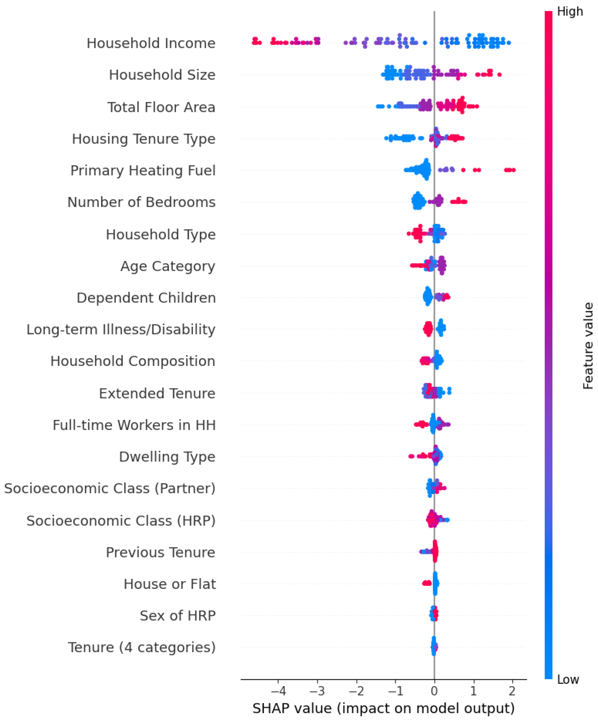
Use SHAP values to enhance model interpretability and assess feature importance.

Census data serves as a valuable resource for energy poverty identification due to its comprehensive demographic, socioeconomic, and housing characteristics, which provide crucial insights into household living conditions [33]. Therefore, this study also investigates the following hypotheses:

• Census data alone has predictive power for energy poverty classification, even without direct energy consumption data.
• Adding more socioeconomic and housing-related proxies (e.g., income, floor area, dwelling type) will improve model accuracy.

Through this methodology, we aim to develop a robust and high-accuracy machine learning model for energy poverty identification. By addressing research gaps, this study contributes to enhancing machine learning applications for energy poverty identification, with implications for policy implementation in the UK.

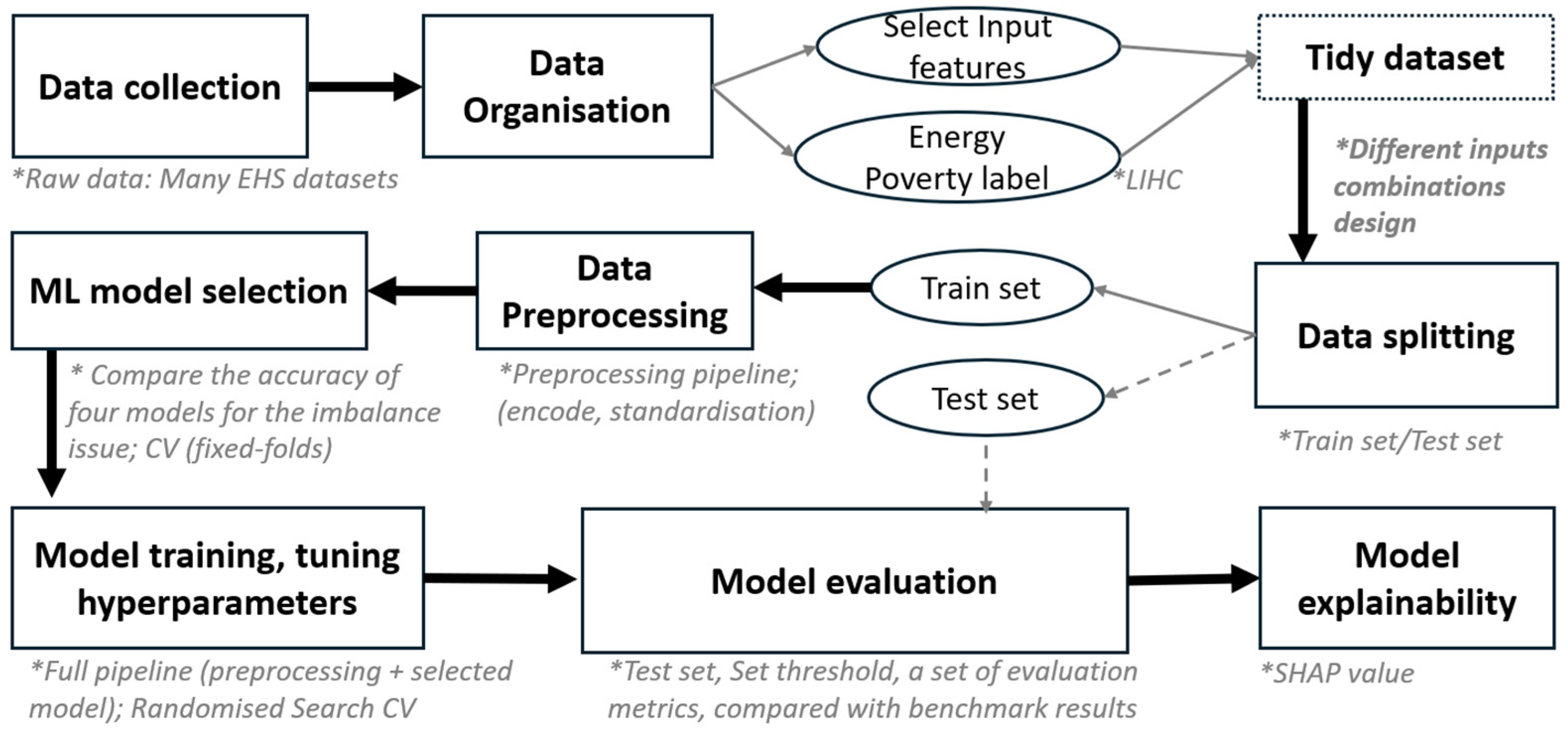
2. Materials and Methods

Our study follows a structured workflow, as illustrated in Figure 2, to develop and evaluate machine learning models for energy poverty identification.

The process begins with data collection and organisation, where household-level data are sourced from the English Housing Survey (EHS). Key variables, including input features and energy poverty labels (LIHC indicator), are selected and processed to form a tidy dataset. To assess the impact of different feature selections, we design two combinations of inputs, each representing a distinct combination of predictors. The dataset is then split into training and test sets, ensuring that the test set is used only once for final evaluation.

During model development, we first apply a preprocessing pipeline, including encoding categorical variables and standardising numerical features to ensure data consistency. To address the class imbalance issue, we compare the performance of four machine learning models using cross-validation (fixed-folds) and select the most suitable model for further training. Hyperparameter tuning is conducted using Randomised Search CV to optimise model performance. After training and hyperparameter tuning, we evaluate the final model on the test set, using a range of performance metrics, including precision and recall. We then compare the predictive accuracy of the models under different input scenarios with a benchmark model.

In the end, to enhance model explainability, we apply SHAP values, identifying the most influential features in energy poverty classification and improving model interpretability. The details of each step are presented in the following subsections.

2.1. Data Collection and Organisation

2.1.1. Input Feature Selection

The first principle guiding our feature selection was to align as closely as possible with the variables used in the benchmark model from UK government. In addition, we prioritised features that were consistent with UK census criteria and supported by the UK energy poverty framework and the existing literature on the key factors related to energy poverty, particularly those related to household income, housing quality, and occupancy characteristics. Therefore, a key challenge was the lack of exact matching data from the administrative sources used in the benchmark model, which utilised government datasets including the official NEED (National Energy Efficiency Data-Framework) [29], Experian [30], Department for Work and Pensions [31], and Ordnance Survey [32]. These data were unavailable in the datasets we had access to. This limitation required us to identify proxy variables from alternative data sources to approximate the missing information. To address this challenge, we used data from EHS [34] as a substitute for census data and the datasets used in the benchmark model to approximate the missing information. The EHS datasets provided rich household-level data, including gross annual income, heating system type, tenure, and household size. These variables met our selection principles and were critical inputs for effective energy poverty classification.

The raw data were collected from the UK Data Service [35] and were originally sourced from the EHS from the following two datasets:

• English Housing Survey, 2021: Housing Stock Data. UK Data Service. SN: 9229 [36];
• English Housing Survey, 2021–2022: Household Data. UK Data Service. SN: 9230 [37].

These collected datasets were linked using a unique identifier for each household, a serial anonymised number. The total datasets included up to 180 variables for 10,527 households, covering demographic, socioeconomic, and housing characteristics. Among the 180 variables, 20 variables were selected as proxies for census data and the datasets used in the benchmark model. These proxy variables were carefully selected to ensure that only relevant and meaningful features were included through domain knowledge filtering. Details, including data mapping methods and variable descriptions, are provided in Appendix A (see

Table A1. Variable name and description used in model development.

Proxy	Variable Name	Description	Value Labels Example
Proxy census data based on criteria through the 2021 Census from the ONS website [72].	hhsizex	Number of persons in the household	1, 2, 3, 4
	sft	Number of full-time workers in household	1, 2, 3, 4
	nssech9	NS-SEC Socioeconomic Classification—HRP	1 “higher managerial and professional occupations”. 2 “lower managerial and professional occupations”.
	nssecp9	NS-SEC Socioeconomic Classification—HRP’s partner	1 “higher managerial and professional occupations”. 2 “lower managerial and professional occupations”.
	hhtype11	Household type—All 11 categories	1 “couple with no child(ren)”. 2 “couple with dependent child(ren) only”.
	ager	Report age categories	1 “16 to 24” 2 “25 to 34” 3 “35 to 44”
	sexhrp	Sex of household reference person	1 “male” 2 “female”
	hhcomp1	Household composition, focussing on HRP (seven categories)	1 “married/cohabiting couple” 2 “lone parent, male HRP” 3 “lone parent, female HRP”
	ndepchild	Number of dependent children in household	1, 2, 3
	hhltsick	Anyone in household with long-term illness or disability	1 “yes” 2 “no”
	tenure2	Tenure group 2	1 “own outright” 2 “buying with mortgage (including shared ownership)” 3 “local authority tenant”
	prevten	Tenure of previous home of HRP	1 “new household” 2 “owned outright” 3 “buying with a mortgage”
	tenex	Extended tenure of household	1 “own with mortgage” 2 “own outright” 3 “privately rent”
	tenure4x	Tenure—Four categories.	1 “owner occupied” 2 “private rented” 3 “local authority” 4 “housing association”
	Bedrqx	Number of bedrooms	1, 2, 3
	fuelx	Type of fuel used for the main or primary space heating system	1 “gas fired system” 2 “oil fired system” 3 “solid fuel fired system” 4 “electrical system”
	DWtype	Dwelling type (eight categories)	1 “small terraced house” 2 “medium/large terraced house” 3 “semi-detached house”
Proxy for other inputs	housex	Whether the dwelling is a house or flat (two categories)	1 “house or bungalow” 2 “flat”
	HYEARGRx	Household gross annual income (inc. income from all adult household members)	100,000.00: “£100,000 or more”
	FloorArea	Total floor area	Numeric

). The selected variables were categorised as follows:

• Census Data Proxies [38,39]: A total of 17 variables representing household composition, socioeconomic classification, and living conditions, including household size, number of dependent children, tenure, long-term illness or disability status, heating fuel type, and detailed dwelling type (eight categories).
• Other Input Proxies: Three variables, including household annual income, total floor area, and dwelling type (two categories: whether household is a house or flat).

These features were used to design different input combinations, each with a distinct set of predictors.

2.1.2. Input Combinations

To investigate the effectiveness of census-based data in identifying energy poverty and to evaluate how incorporating additional variables enhances the performance of the benchmark model, we design two different combinations of predictors with varying levels of input complexity.

• Combination 1 (census-only): This combination assesses the standalone predictive capability of census data in identifying energy poverty. This model is named “COM-1” in the analysis.
• Combination 2 (census + other inputs): Expands Combination 1 by incorporating additional proxies. Notably, floor area and dwelling type (two categories) can be obtained from Building 3D Modelling Lab [40], highlighting the potential for using these accessible data sources as predictive inputs, while (estimated) household income can be obtained from companies such as Experian. This model is named “COM-2” in the analysis.

Based on these two input combinations, two models are developed, and their performance is evaluated against the benchmark model. By comparing results across different predictor sets, we assess the trade-offs between model complexity, predictive performance, and data accessibility for energy poverty identification. Critically, in the benchmark model, actual annual energy consumption data from the NEED dataset is used as an input. However, it is important to note that we do not have access to real-time or household-specific gas and electricity usage data. Consequently, the gas and electricity usage data are not included here. Instead, we conduct an additional model training where all available variables (census and other inputs), along with SAP values, are used as model inputs to assess performance. In the UK, the SAP value reflects the energy efficiency of a dwelling [41]; therefore, it serves as a proxy for estimating household energy demand. The results from this additional model are provided in the Appendix (see content related to the keyword “Extended Model”). This “Extended Model”, which includes additional features, as described in Appendix, is provided as a supplementary performance analysis alongside the benchmarks and other models presented in the main text.

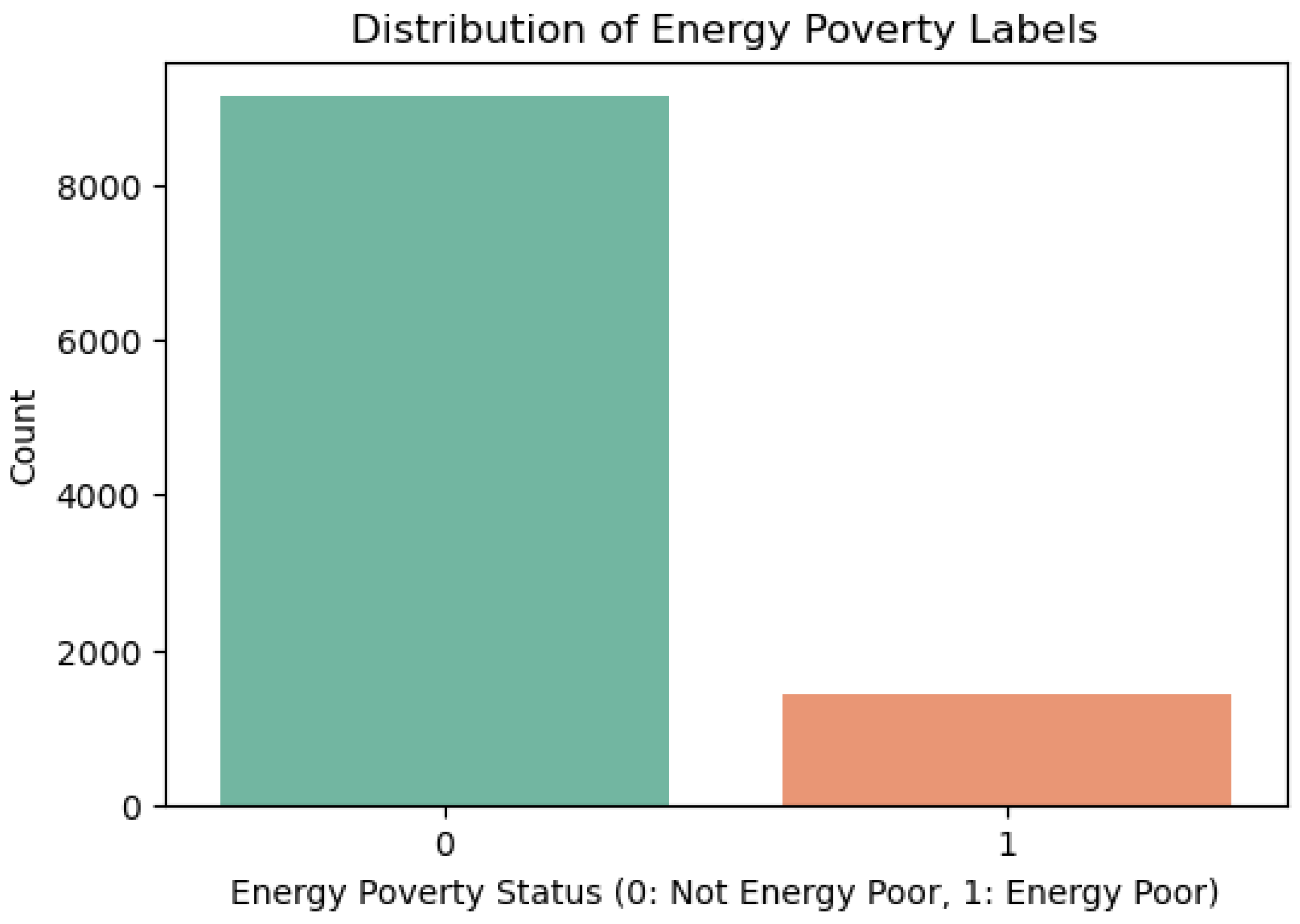
2.1.3. Energy Poverty Label

To obtain energy poverty labels, we use the energy poverty dataset 2021 from the EHS: Department for Business, Energy & Industrial Strategy (2024). English Housing Survey: Fuel Poverty Dataset, 2021. UK Data Service. SN: 9243 [42].

While this dataset provides the LILEE indicator, our study requires alignment with the benchmark model, which uses the LIHC indicator, to ensure consistency in energy poverty definitions. Therefore, we calculate the LIHC label following the official methodology from the Fuel Poverty Methodology Handbook 2020 [43] and need data that is available in the energy poverty datasets. The LIHC indicator defines energy-poor households as those with below-threshold income and energy costs above the national median. In practice, this requires computing household equivalised income and modelled energy costs, and comparing them against national-level thresholds [43]. According to this definition, a household is classified as fuel-poor under LIHC in the following cases:

• High Cost: The household’s equivalised fuel costs exceed the national median.
• Low Income: The household’s equivalised after-housing-cost (AHC) income falls below an adjusted threshold.

To compute this, we extract fuel expenditure, equivalisation factors, and AHC income variables from the dataset and apply the LIHC methodology. As shown by Figure 3, among the overall 10,527 households, 9140 are not energy-poor, and 1432 (around 14%) are identified as energy-poor households. We can see that the ratio between non-energy-poor and energy-poor households is about 6:1, which means this energy poverty dataset is imbalanced.

The full calculation process and the implementation code are available (see the “Data Availability Statement”) to ensure transparency and reproducibility.

2.2. Data Splitting and Preprocessing Pipeline

After obtaining a tidy dataset containing input features and energy poverty labels, the dataset is split into training (75%) and test (25%) sets. This ensures that the model is trained on a sufficient amount of data while keeping a separate portion for final model evaluation. The training set is used exclusively for model development, whereas the test set is only used in the final model evaluation. Due to the dataset containing both numerical and categorical variables, a data preprocessing pipeline is implemented to handle data standardisation [44] and encoding [45]:

• Numerical variables: We apply data standardisation using StandardScaler [46], which transforms features to have a mean of zero and a standard deviation of one. Standardisation ensures that numerical variables with different scales do not disproportionately influence the model.
• Categorical variables: We use One-Hot Encoding [47], which converts categorical features into a binary format, allowing machine learning models to process them effectively. This method prevents the model from misinterpreting categorical values as ordinal relationships, preserving the integrity of categorical data.

Using a pipeline-based approach [48] streamlines the preprocessing steps, ensuring consistency across training and evaluation while preventing data leakage. By integrating encoding and scaling into a single pipeline, we enhance reproducibility and maintain a structured workflow.

2.3. Machine Learning Model Selection

The objective of the machine learning model selection is to compare the performance of the different models, RF and XGBoosting, while applying different techniques to handle class imbalance, including undersampling and class weighting. The RF and XGBoosting models are widely used for classification tasks and have been applied in previous studies on machine-learning-based energy poverty prediction, such as [6,17,18,21,22,23]. RF is a bagging-based method that builds multiple Decision Trees and aggregates their outputs to improve generalisation and reduce overfitting [49]. XGBoosting is a gradient boosting algorithm that sequentially refines weak learners, optimising performance through gradient-based updates [49].

When using machine learning to predict energy poverty, class imbalance poses a critical challenge [50], as models tend to learn from the majority class (not fuel-poor houses), leading to poor performance in identifying fuel-poor households. Without addressing this issue, the model may perform well overall but will struggle to correctly classify energy-poor households, leading to a biassed prediction that underestimates the actual energy poverty. To address this, we apply the resampling [51] and class weight adjustment [52,53] techniques for RF and XGBoosting, respectively, resulting in four models. The four models are evaluated to determine the most suitable one for handling class imbalance before proceeding to further training and hyperparameter tuning.

• Resampling techniques: We apply Random Undersampling before training to reduce the bias towards the majority class. Undersampling techniques are used for reducing the imbalance ratio by removing samples from the majority class [54]. This approach helps balance class representation, ensuring that the model does not disproportionately prioritise the majority class, thereby improving its ability to identify energy-poor houses.
• Class weight adjustment: Another effective approach is adjusting class weights in the model’s cost function, assigning higher weights to the minority class to make misclassification more costly and to improve recall for fuel-poor households [55]. For RF, we set class weight as “balanced”, which automatically assigns weights to be inversely proportional to class frequencies, reducing bias toward the majority class. For XGBoost, we adjust the algorithms with the scale pos weight parameter, which is typically calculated as the ratio of the number of negative samples to the number of positive samples in the training data. This adjustment ensures that the model gives sufficient importance to the minority class, enhancing its ability to correctly identify fuel-poor households.

We use CV (k = 5) and compare both accuracy and balanced accuracy across the four models. CV is a robust technique for assessing model generalisation by repeatedly partitioning the training dataset and measuring the average performance across multiple subsets [56]. The dataset is split into k folds. The model is trained on k-1 folds and validated on the remaining folds, repeating this process k times. The final performance is averaged across all folds.

We use both accuracy and balanced accuracy as metrics of performance for handling imbalance issues. Accuracy measures the proportion of correctly classified instances out of all instances, but it can be misleading in imbalanced datasets where the majority class dominates [24]. Balanced accuracy, on the other hand, ensures that performance is fairly evaluated across both majority and minority classes [57]. The detailed explanation of accuracy and balanced accuracy are available in Section 2.5. By comparing accuracy and balanced accuracy, we select the most appropriate model that effectively handles class imbalance while maintaining strong overall predictive performance and that could be used for further training.

2.4. Model Training and Hyperparameter Tuning

After selecting the most appropriate model that could handle the imbalance issue, we applied hyperparameter tuning to optimise model performance and utilise 5-fold Randomised Search Cross-Validation (RandomizedSearchCV). This method randomly selects a subset of hyperparameter combinations [58]. These hyperparameters include colsample_bytree, gamma, learning_rate, max_depth, n_estimators, reg_alpha & reg_lambda, and subsample. The detailed explanation of these hyperparameters is available in Appendix B. Each selected combination is evaluated using k-fold CV. The best-performing hyperparameter set was chosen based on the evaluation metric that was the highest balanced accuracy score obtained during cross-validation. [59]. This training and tuning approach ensured that the model was well-optimised. The details of hyperparameter tuning, including the type of hyperparameters tuned and the results, are available in Appendix B (

Table A2. Hyperparameter results.

Hyperparameter	COM-1	COM-2	Extended Model
colsample_bytree	0.70	0.69	0.96
gamma	4.68	4.68	4.04
learning_rate	0.05	0.05	0.2
max_depth	11	11	8
n_estimators	250	250	383
reg_alpha	5.4	8.04	8.04
reg_lambda	6.96	6.96	1.87
subsample	0.61	0.61	0.95

).

2.5. Model Evaluation and Explainability

We use multiple evaluation metrics to ensure a comprehensive assessment of the models [60], including the following:

• Accuracy: Measures the proportion of correctly classified households.

$$Accuracy={\displaystyle \frac{TP+TN}{TP+TN+FP+FN}}$$

(1)

where

$TP$ = True Positive;

$TN$ = True Negative;

$FP$ = False Positive;

$FN$ = False Negative.

• Precision: Indicates how many of the predicted fuel-poor households are actually fuel-poor.

$$Precision={\displaystyle \frac{TP}{TP+FP}}$$

(2)

• Recall (Sensitivity, True Positive Rate): Measures the proportion of actual fuel-poor households correctly identified by the model. A higher recall ensures fewer False Negatives.

$$Recall={\displaystyle \frac{TP}{TP+FN}}$$

(3)

• F1-Score: Represents the harmonic mean of precision and recall, providing a balanced measure of model performance.

$$F1=2\times {\displaystyle \frac{Precision\times Recall}{Precision+Recall}}$$

(4)

• Balanced Accuracy: Measures both the model’s sensitivity (True Positive Rate) and specificity (True Negative Rate).

$$Balanced Accruacy={\displaystyle \frac{1}{2}}\times (Recall+{\displaystyle \frac{TN}{TN+FP}})$$

(5)

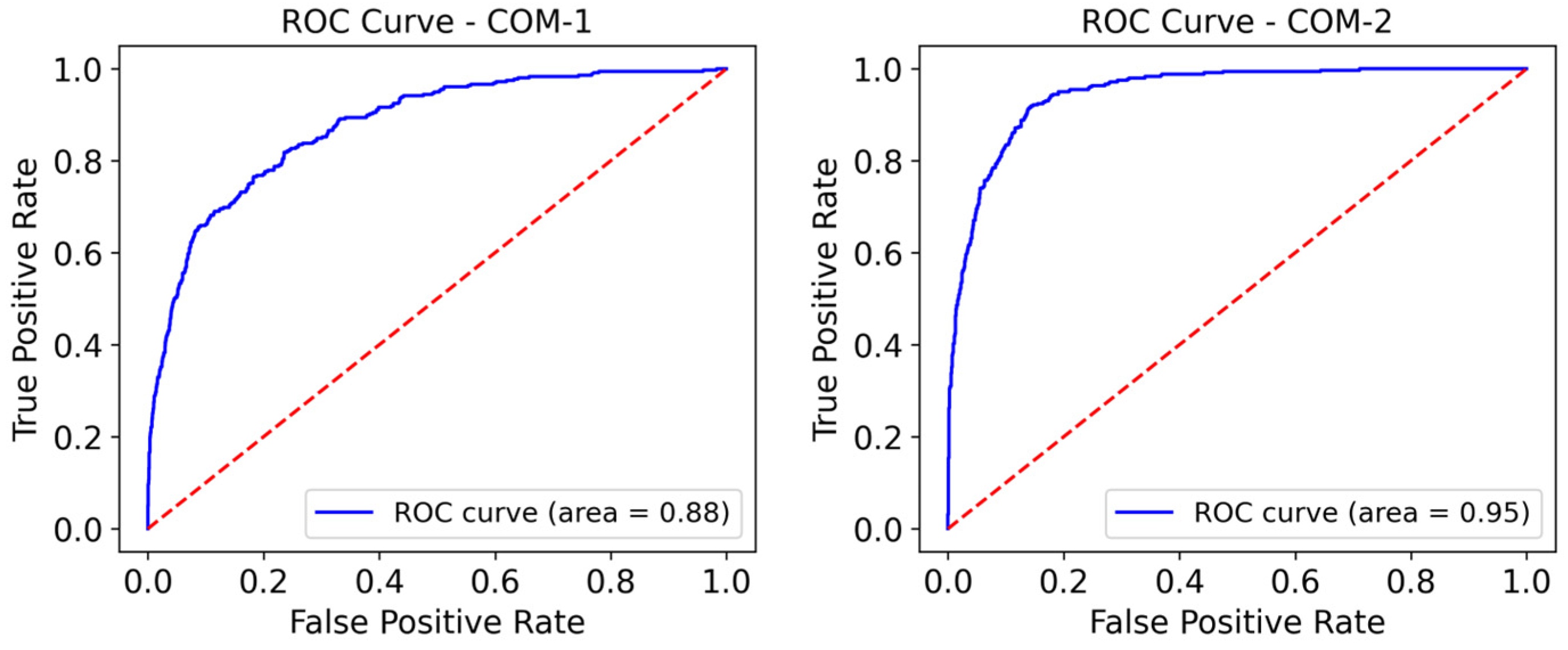
• ROC and AUC (Area Under Curve): The ROC (Receiver Operating Characteristic) curve plots the trade-off between a model’s recall (True Positive Rate) and False Positive Rate (FPR) at different classification thresholds:

$$FPR={\displaystyle \frac{FP}{FP+TN}}$$

(6)

The AUC represents the area under the curve. It represents the probability that a randomly chosen energy-poor household is ranked higher than a randomly chosen non-energy-poor household. This metric evaluates the overall performance of a binary classifier across all possible thresholds. A higher AUC value (closer to 1) indicates better performance. An AUC of 0.5 indicates no better performance than random choice.

These metrics also allow for a detailed comparison between our models and the benchmark. The confusion matrix is used also used, which is a cross-tabulation that consists of a combination of metric results [25]. To further enhance the interpretability of the best-performing model, we calculate SHAP values. SHAP values provide the following [19,61]:

• Feature Importance: Identifying which input features contribute the most to predicting energy poverty.
• Local Interpretability: Explaining individual household predictions, allowing insights into why certain households are classified as energy-poor.
• Fairness Assessment: Ensuring that predictions align with logical socioeconomic and housing-related indicators rather than arbitrary biases.

By leveraging SHAP value analysis, we ensure that our model is not only accurate but also transparent and explainable.

3. Results

3.1. Machine Learning Approach Selection

The results of the approach are presented in

Table 2. Model performance for handling class imbalances.

Machine Learning Models	COM-1		COM-2
	Accuracy	Balanced Accuracy	Accuracy	Balanced Accuracy
RF + undersampling	0.78	0.78	0.86	0.87
RF + class weight	0.78	0.78	0.86	0.87
XGBoost + undersampling	0.78	0.78	0.87	0.87
XGBoost + (scale_pos_weight)	0.82	0.78	0.90	0.87

, which compares the performance of different models in handling class imbalances across the two input combinations (COM-1, COM-2).

The results from Table 2 show that XGBoost with scale_pos_weight consistently, across the cross-validation folds, outperforms all other models across all input combinations (COM-1, COM-2), achieving the highest balanced accuracy and accuracy. This makes it the best-performing model for addressing class imbalance, demonstrating a superior capability in identifying energy-poor households while maintaining a strong overall predictive performance.

Since these results are obtained through CV, they provide a reliable assessment of the model’s generalisation ability. Therefore, for further model development, we select XGBoost with scale_pos_weight adjustment for model training, hyperparameter tuning, and final evaluation. The final hyperparameter tuning results for all models are presented in Appendix B.

3.2. Models Performance Metrics

As illustrated in Figure 4, the performance of the machine learning models is assessed using precision, recall, F1-score, accuracy, and balanced accuracy. The benchmark model, which serves as a reference, achieves a recall of 0.90, indicating a strong ability to capture actual energy-poor households. When setting the decision threshold to maintain a similar recall across models, it is observed that two models (COM-1, COM-2) demonstrate high recall values (0.90 and 0.91) close to the benchmark model, confirming their capability in identifying energy-poor households.

Despite the high recall performance, the two models outperform the benchmark model in precision, F1-score, accuracy, and balanced accuracy, highlighting their improved predictive performance. COM-1, which relies only on census-based data, already achieves comparable performance to the benchmark model, suggesting that census data alone holds significant predictive power for energy poverty identification. However, the COM-2 model further enhances model performance.

The results indicate that COM-2, while maintaining a recall similar to the benchmark, achieves notable improvements in precision and F1-score. In particular, precision improves from 0.24 (benchmark and COM-1) to 0.51 (COM-2). This increase suggests that incorporating additional variables reduces False Positive classifications, making the models more effective in accurately identifying truly energy-poor households. Similarly, F1-score increases from 0.37 (benchmark) to 0.65 (COM-2), demonstrating that adding more predictors results in a better balance between precision and recall.

Accuracy and balanced accuracy also exhibit steady improvements across the models. The benchmark model achieves an accuracy of 0.67 and a balanced accuracy of 0.77, whereas COM-2, the best-performing model, reaches 0.87 and 0.88 for accuracy and balanced accuracy, respectively.

The confusion matrix results (see Appendix C (

Table A3. The confusion matrix results for all models, respectively.

COM-1
Set Threshold = 0.23
Classification	Precision	Recall	F1-Score	Support
Not Energy-Poor	0.98	0.61	0.70	2285
Energy-Poor	0.27	0.90	0.41	358
Accuracy			0.65	2643
Macro Avg	0.62	0.76	0.58	2643
Weighted Avg	0.88	0.65	0.70	2643
balanced accuracy = 0.76, ROC curve (area = 0.88)
COM-2
Set Threshold = 0.45
Classification	Precision	Recall	F1-Score	Support
Not Energy-Poor	0.98	0.86	0.92	2285
Energy-Poor	0.51	0.91	0.65	358
Accuracy			0.87	2643
Macro Avg	0.75	0.88	0.79	2643
Weighted Avg	0.92	0.87	0.88	2643
balanced accuracy = 0.88, ROC curve (area = 0.95)
Extended Model (Add SAP Value)
Set Threshold = 0.43
Classification	Precision	Recall	F1-Score	Support
Not Energy-Poor	0.98	0.88	0.93	2285
Energy-Poor	0.56	0.90	0.69	358
Accuracy			0.89	2643
Macro Avg	0.77	0.89	0.81	2643
Weighted Avg	0.92	0.89	0.90	2643
balanced accuracy = 0.90, ROC curve (area = 0.96)
Benchmark Model
Classification	Precision	Recall	F1-Score	Support
Not Energy-Poor	0.98	0.64	0.77	2396
Energy-Poor	0.24	0.90	0.37	296
Accuracy			0.67	2692
Macro Averaged	0.61	0.77	0.57	2692
Weighted Averaged	0.90	0.67	0.74	2692
balanced accuracy = 0.77, ROC curve (area = 0.89)

)) for the two proposed models (COM-1, COM-2) are presented alongside the benchmark model and Extended Model, summarising their prediction performance for both energy-poor and non-energy-poor households. Compared to the benchmark model, all proposed models achieve a higher model performance, suggesting that integrating additional administrative data enhances predictive performance.

The overall results support our hypotheses that (1) census data alone can be effective in predicting energy poverty, and (2) incorporating more administrative data could enhance predictive performance.

3.3. Models’ ROC Curve and AUC Value

Figure 5 presents the ROC curves for the two models, illustrating their ability to distinguish between fuel-poor and non-fuel-poor households across different classification thresholds. AUC values further confirm the trend observed in the performance metrics. COM-1 achieves an AUC of 0.88, while COM-2 demonstrates improved discrimination abilities with an AUC value of 0.95.

The increase in the AUC from model COM-1 to COM-2 indicates that incorporating additional predictive variables enhances the model’s ability to differentiate between classes, reducing both False Positives and False Negatives. The results suggest that while census data alone can provide a baseline predictive capability, the inclusion of housing characteristics and income predictors significantly refines model performance. The highest-performing model, COM-2, achieves an AUC of 0.95, reinforcing its superior predictive power. This highlights the potential for integrating administrative data into future predictive models for energy poverty identification.

3.4. SHAP Value of the Best Performance Model

The SHAP summary plot (see Figure 6) provides insight into the most influential factors affecting energy poverty classification in the COM-2 model. The x-axis represents the SHAP value, which measures how much each feature influences the model’s prediction. Negative SHAP values (left) mean the feature reduces the likelihood of being classified as energy-poor. Positive SHAP values (right) mean the feature increases the likelihood of being classified as energy-poor. The y-axis lists the features ranked by their importance, with the most influential features at the top. The spread of dots across the x-axis shows variability, indicating how different households are impacted differently by the same feature.

The SHAP value result highlights that household income is the most influential factor in energy poverty identification. Lower income households are significantly more likely to be classified as energy-poor, aligning with the existing literature on energy vulnerability. Household size and total floor area also play crucial roles, with larger households facing increased energy demands. The detailed housing tenure type (eight categories) further contributes to disparities, as renters experience greater energy vulnerability compared to homeowners. These methods suggest a machine learning model, enhanced by SHAP, could provide interpretable results regarding the key drivers of energy poverty.

4. Discussion and Limitations

4.1. Discussion

The findings of this study emphasise the opportunity to integrate machine learning into energy poverty identification to enhance efficiency, scalability, and policy effectiveness. The UK government’s methodology for identifying energy poverty, as outlined in the Fuel Poverty Methodology Handbook [10], relies on extensive data collection. While theoretically robust for measuring fuel poverty, this approach introduces significant practical challenges for implementing this indicator for the identification of fuel poverty in specific households. Many households may not have easily available or up-to-date information on income from benefits, tax credits, savings, council tax support, fuel prices, energy consumption, or housing-related expenses. Data collection is complex and time-consuming, limiting the feasibility of large-scale energy poverty identification and in-time policy implementation.

In contrast, the machine learning model developed in this study demonstrates that energy poverty can be effectively identified using a more limited and accessible dataset, even outperforming the benchmark model. By incorporating only a few features based on census data and other factors, including gross annual household income, total floor area, and dwelling type, the model achieves better-than-benchmark performance. This suggests that machine learning approaches can provide a viable alternative, offering a more scalable and efficient method for identifying fuel-poor households without requiring excessive data collection. Our findings are consistent with previous studies suggesting that machine learning models and socioeconomic data have the potential to improve the energy poverty targeting efficiency compared to traditional approaches [6,17,23]. In particular, our results support the applicability of such methods in the UK context. Unlike indicator-based methods, our ML framework offers scalable adaptability to changing data environments and can integrate local administrative datasets with minimal structural modification. The comparison between the traditional method and the machine learning approach is presented in the

Table 3. Comparison between the traditional method and the machine learning approach.

Aspect	Traditional Method	Machine Learning Approach
Data Requirement	Extensive data collection (AHC income, fuel costs, energy needs, housing expenses, etc.)	Minimal and accessible (household income, SAP score, census data, floor area)
Computational Efficiency	Time-consuming manual collection and calculations	Automated predictions with efficient computation
Scalability	Limited scalability due to complex data requirements	Highly scalable due to reduced data dependency
Accuracy	Reliable but constrained by data availability	Comparable or better-than-benchmark performance
Interpretability	Fixed rule-based approach, difficult to break down individual household-level factors	SHAP values show the contribution of each feature to an individual household’s classification
Handling of Non-Linearity	Assumes a fixed income–energy cost threshold, ignoring non-linear relationships	Capture complex interactions between income, housing, and energy efficiency
Household-Level Insights	Provides only a binary classification (energy-poor or not) based on predefined thresholds	Analysis at the individual household level, revealing why specific households are energy-poor
Policy Implications	Requires detailed household-level data, limiting rapid assessments	Enables faster, data-driven decisions, even in data-limited contexts
Future Application	Static methodology with limited adaptability	Can integrate smart meter data to measure and identify energy poverty more dynamically and comprehensively

below:

For the UK government, adopting machine learning for energy poverty identification can enhance policy efficiency and effectiveness. By leveraging existing administrative data sources such as census data and the amount of historical energy poverty classifications as ground truth, the government can train predictive models that provide timely and scalable assessments of energy poverty risk. This machine learning model could be used to achieve the following:

• Enhance rapid assessments of energy poverty using readily available datasets without the need for direct household surveys or complex financial data collection.
• Support local authorities and policymakers in designing targeted interventions by identifying households most at risk, enabling data-driven decision-making for financial aid distribution and energy efficiency programmes.
• Facilitate real-time monitoring of energy vulnerability trends by integrating additional real-world data sources, such as smart meter consumption, energy tariffs, and weather data, to track changes in household energy usage patterns over time, allowing the early detection of households struggling with energy costs or dynamically updating its predictions to reflect changing economic and environmental conditions.
• By identifying at-risk households before they fall into severe fuel poverty, social programmes can be more preventative rather than reactive, leading to better long-term outcomes.

Additionally, integrating smart meter consumption data in the future could further enhance the predictive power of machine learning models, allowing for real-time monitoring of energy vulnerability and enabling more proactive policy interventions. Notably, ongoing research from the Smart Energy Research Lab (SERL) is already advancing this area [62,63,64]. The proposed ML framework could be integrated with emerging smart energy systems to support targeted demand-side interventions. For instance, linking predictive models to smart grid infrastructure could enable the real-time identification of vulnerable households for demand response, dynamic pricing protection, or automated energy support services. Intelligent Energy Management Systems [65] could leverage such predictions to allocate renewable energy or efficiency upgrades more equitably. The outputs of our model could also inform microsimulation models or macroeconomic analyses that evaluate the distributional impact of policy interventions, such as subsidies or energy rebates. By identifying the households most at risk, economic models can assess whether current support schemes are cost-effective and equitably targeted, helping to design more efficient policy instruments. All these insights suggest that using existing administrative data and AI-driven methodologies could significantly improve energy poverty identification, aligning with national goals.

While the primary focus of this study is on household energy poverty in the UK, we briefly explore the potential extrapolations of our methodological framework to illustrate its broader relevance across domains. Beyond energy poverty, our framework, which is based on linking administrative datasets with machine learning classification models, can be extended to contexts where identifying spatial or socioeconomic vulnerability is essential. For instance, in the extractive or mining industries, where socioeconomic factors are closely linked to regional impacts and compensation schemes [66,67], our proposed approach and framework could inform the more equitable distribution of royalties or salaries based on regional deprivation indices, aligning with findings from previous studies like [68,69]. Similarly, targeted resource allocation policies, such as electricity pricing strategies or infrastructure investments in underdeveloped areas, may benefit from data-driven socioeconomic profiling using our methods. However, it is crucial to acknowledge that the application of such predictive models in sensitive domains raises ethical concerns, including issues of fairness, transparency, and the risk of reinforcing existing biases. Appropriate governance frameworks must therefore accompany future applications to ensure responsible use.

This approach can also be adapted to other countries or regions with similar limitations in direct energy poverty data, provided administrative datasets are available at the household or regional level. Countries with census, welfare, and housing energy records can replicate the methodology by adjusting variable mapping and model training to local contexts. However, such applications must carefully consider context-specific ethical and governance concerns. Consequently, given the use of sensitive socioeconomic and housing data, it is important to consider ethical safeguards in both model development and deployment. While data is anonymised, privacy risks must be managed through secure handling and strict access protocols. Additionally, fairness audits are necessary to ensure that ML predictions do not systematically disadvantage certain groups. We recommend incorporating bias evaluation metrics and participatory policy design when implementing ML-based targeting in practice.

4.2. Limitations

While our study demonstrates the potential of machine learning for energy poverty identification, several limitations must be acknowledged.

(1)

Trade-offs between model simplicity and predictive accuracy

The machine learning model relies on a reduced set of input features compared to traditional identifying methods. Although the model performs comparably or better than the benchmark, removing certain economic and fuel cost components may introduce unobserved biases. Further research is needed to assess how feature simplifications impact predictive reliability across different socioeconomic groups and geographic regions. Future work could explore hybrid models that balance interpretability with a more comprehensive feature set.

(2)

Limitations of census and administrative data

A major challenge in using census data is its low temporal resolution; it is typically updated once every ten years. This delayed update cycle may fail to capture short-term economic shocks, household transitions, or sudden changes in energy affordability, limiting the model’s ability to reflect real-time energy poverty trends. Similarly, administrative datasets (e.g., housing tenure records) may lack real-time identification.

(3)

Integration of energy consumption and smart meter data

Unlike the benchmark model, this study does not incorporate annual or any real time energy consumption data, which could significantly enhance model adaptiveness and responsiveness. To mitigate this, future work could integrate smart meter data (e.g., from Smart Energy Research Lab (SERL) [70], NEED [29], or other similar resources) where available, allowing for the dynamic updating of predictions. By incorporating energy tariff data, seasonal variations, and consumption behaviours, machine learning models could improve real-time energy vulnerability detection and enable more proactive interventions.

(4)

Ethical considerations and model transparency

As with all machine learning models applied to social welfare contexts, ensuring fairness, transparency, and accountability is crucial. While SHAP values provide insights into feature importance, further work is needed to assess potential biases in the model, particularly in low-data households or underrepresented communities. The potential risks of algorithmic bias and over-reliance on historical administrative records should be carefully evaluated.

(5)

Proxy variables rather than actual administrative datasets

We use proxy variables to approximate key socioeconomic and housing characteristics, as actual census data is not directly available. While these proxies capture relevant trends, they may not fully represent the complexity of real census data. Future studies should explore the use of official census datasets to enhance the accuracy and generalisability of predictions.

(6)

Algorithmic bias

Algorithmic bias remains a significant concern when applying machine learning to socioeconomic datasets, as it can raise ethical and fairness issues [71]. For example, if training data underrepresents certain populations such as low-income or rural households, the model may misclassify these groups and exacerbate existing inequalities. While our modelling pipeline includes stratified sampling to reduce such risks, we recommend that future applications incorporate bias audits, fairness metrics, and stakeholder engagement to promote equitable outcomes.

5. Conclusions

This study demonstrates the potential of machine learning models to enhance the efficiency, scalability, and accessibility of energy poverty identification. By using administrative data, including census-based housing characteristics, and other factors, including household income, floor area, and dwelling type, the model achieves comparable or superior performance to the traditional energy poverty identification method and benchmark machine learning model. These findings highlight the potential of machine learning, enabling faster and more cost-effective energy poverty identification. The key insights are as follows:

(1)

Machine learning offers a data-driven approach to the identification of energy poverty in specific households.

(2)

Census data has predictive power for energy poverty identification. Using a set of administrative features as the input, our best performing machine learning model can identify 91% of energy-poor households, with 51% of predicted energy-poor households actually being energy-poor, a superior performance compared to the benchmark model.

(3)

Policymakers can benefit from integrating machine-learning-based models into energy poverty identification frameworks.

Future research should explore the following: (1) Validating model performance across diverse household demographics and geographic regions, ensuring robustness across different socioeconomic conditions. (2) Integrating more input features, such as real-time energy usage data (e.g., smart meters) or actual annual energy consumption to enhance predictive accuracy. Furthermore, future research could build upon our findings by developing targeted intervention strategies based on the specific causes of energy poverty identified through our models. For example, those facing sudden income shocks may require direct financial assistance. Additionally, by integrating temporal updates and tracking household-level dynamics over time, the framework could be extended to identify households at risk of falling into energy poverty, enabling the design of preventive measures. Such early-warning systems would be critical in reducing long-term vulnerability and enhancing the resilience of vulnerable communities.

References

1. Moore, R. Definitions of fuel poverty: Implications for policy. Energy Policy 2012, 49, 19–26. [Google Scholar] [CrossRef]
2. Waddams Price, C.; Brazier, K.; Wang, W. Objective and subjective measures of fuel poverty. Energy Policy 2012, 49, 33–39. [Google Scholar] [CrossRef]
3. Steve, P.; Audrey, D. Energy Poverty and Vulnerable Consumers in the Energy Sector Across the EU: Analysis of Policies and Measures; Policy Report: European Commission for Energy, Climate Change, Environment; European Commission: Brussels, Belgium, 2015.
4. Bentley, R.; Daniel, L.; Li, Y.; Baker, E.; Li, A. The effect of energy poverty on mental health, cardiovascular disease and respiratory health: A longitudinal analysis. Lancet Reg. Health—West. Pac. 2023, 35, 100734. [Google Scholar] [CrossRef] [PubMed]
5. Huebner, G.M.; Hanmer, C.; Zapata-Webborn, E.; Pullinger, M.; McKenna, E.J.; Few, J.; Elam, S.; Oreszczyn, T. Self-reported energy use behaviour changed significantly during the cost-of-living crisis in winter 2022/23: Insights from cross-sectional and longitudinal surveys in Great Britain. Sci. Rep. 2023, 13, 21683. [Google Scholar] [CrossRef]
6. Al Kez, D.; Foley, A.; Abdul, Z.K.; Del Rio, D.F. Energy poverty prediction in the United Kingdom: A machine learning approach. Energy Policy 2024, 184, 113909. [Google Scholar] [CrossRef]
7. Annual Fuel Poverty Statistics Report: 2024. GOVUK. Available online: https://www.gov.uk/government/statistics/annual-fuel-poverty-statistics-report-2024 (accessed on 12 March 2025).
8. A Critical Analysis of the New Politics of Fuel Poverty in England—Lucie Middlemiss. 2017. Available online: https://journals.sagepub.com/doi/full/10.1177/0261018316674851 (accessed on 29 August 2024).
9. Sovacool, B.K. Fuel poverty, affordability, and energy justice in England: Policy insights from the Warm Front Program. Energy 2015, 93, 361–371. [Google Scholar] [CrossRef]
10. Fuel Poverty Statistics Methodology Handbooks. GOVUK. 2024. Available online: https://www.gov.uk/government/publications/fuel-poverty-statistics-methodology-handbook (accessed on 13 February 2025).
11. Committee on Fuel Poverty Annual Report: 2024. GOVUK. Available online: https://www.gov.uk/government/publications/committee-on-fuel-poverty-annual-report-2024 (accessed on 3 October 2024).
12. Better Use of Data and AI in Delivering Benefits to the Fuel Poor: Research Report and CFP’s Recommendations. GOVUK. Available online: https://www.gov.uk/government/publications/better-use-of-data-and-ai-in-delivering-benefits-to-the-fuel-poor-research-report-and-cfps-recommendations (accessed on 13 February 2025).
13. Homepage|SocialWatt. Available online: https://www.socialwatt.eu/en (accessed on 12 March 2025).
14. ENPOR. IEECP. Available online: https://ieecp.org/projects/enpor/ (accessed on 12 March 2025).
15. Department for Business, Energy & Industrial Strategy (BEIS). Machine Learning and Fuel Poverty Targeting: Annex A. 2017. Available online: https://assets.publishing.service.gov.uk/media/5a823bc5e5274a2e87dc1d8c/need-framework-annex-a-fuel-poverty-targeting.pdf (accessed on 2 December 2024).
16. Ghorbany, S.; Hu, M.; Yao, S.; Wang, C.; Nguyen, Q.C.; Yue, X.; Alirezaei, M.; Tasdizen, T.; Sisk, M. Examining the role of passive design indicators in energy burden reduction: Insights from a machine learning and deep learning approach. Build. Environ. 2024, 250, 111126. [Google Scholar] [CrossRef] [PubMed]
17. Spandagos, C.; Tovar Reaños, M.A.; Lynch, M.Á. Energy poverty prediction and effective targeting for just transitions with machine learning. Energy Econ. 2023, 128, 107131. [Google Scholar] [CrossRef]
18. Mukelabai, M.D.; Wijayantha, K.G.U.; Blanchard, R.E. Using machine learning to expound energy poverty in the global south: Understanding and predicting access to cooking with clean energy. Energy AI 2023, 14, 100290. [Google Scholar] [CrossRef]
19. van Hove, W.; Dalla Longa, F.; van der Zwaan, B. Identifying predictors for energy poverty in Europe using machine learning. Energy Build. 2022, 264, 112064. [Google Scholar] [CrossRef]
20. Abbas, K.; Butt, K.M.; Xu, D.; Ali, M.; Baz, K.; Kharl, S.H.; Ahmed, M. Measurements and determinants of extreme multidimensional energy poverty using machine learning. Energy 2022, 251, 123977. [Google Scholar] [CrossRef]
21. Dalla Longa, F.; Sweerts, B.; van der Zwaan, B. Exploring the complex origins of energy poverty in The Netherlands with machine learning. Energy Policy 2021, 156, 112373. [Google Scholar] [CrossRef]
22. Wang, H.; Maruejols, L.; Yu, X. Predicting energy poverty with combinations of remote-sensing and socioeconomic survey data in India: Evidence from machine learning. Energy Econ. 2021, 102, 105510. [Google Scholar] [CrossRef]
23. Hong, Z.; Park, I.K. Comparative Analysis of Energy Poverty Prediction Models Using Machine Learning Algorithms. J. Korea Plan. Assoc. 2021, 56, 239–255. [Google Scholar] [CrossRef]
24. Thölke, P.; Mantilla-Ramos, Y.-J.; Abdelhedi, H.; Maschke, C.; Dehgan, A.; Harel, Y.; Kemtur, A.; Mekki Berrada, L.; Sahraoui, M.; Young, T.; et al. Class imbalance should not throw you off balance: Choosing the right classifiers and performance metrics for brain decoding with imbalanced data. NeuroImage 2023, 277, 120253. [Google Scholar] [CrossRef] [PubMed]
25. Owusu-Adjei, M.; Ben Hayfron-Acquah, J.; Frimpong, T.; Abdul-Salaam, G. Imbalanced class distribution and performance evaluation metrics: A systematic review of prediction accuracy for determining model performance in healthcare systems. PLoS Digit. Health 2023, 2, e0000290. [Google Scholar] [CrossRef]
26. Machine Learning and Synthetic Minority Oversampling Techniques for Imbalanced Data: Improving Machine Failure Prediction. Comput. Mater. Contin. 2023, 75, 4821–4841. [CrossRef]
27. Lee, W.; Seo, K. Downsampling for Binary Classification with a Highly Imbalanced Dataset Using Active Learning. Big Data Res. 2022, 28, 100314. [Google Scholar] [CrossRef]
28. What Is Administrative Data?—ADR UK. Available online: https://www.adruk.org/our-mission/administrative-data/ (accessed on 13 February 2025).
29. National Energy Efficiency Data-Framework (NEED). GOVUK. 2024. Available online: https://www.gov.uk/government/collections/national-energy-efficiency-data-need-framework (accessed on 10 March 2025).
30. Data Sets|Experian Business. Experian Product Database 2024. Available online: https://www.experian.co.uk/business-products/data-sets/ (accessed on 10 March 2025).
31. Department for Work and Pensions. GOVUK 2025. Available online: https://www.gov.uk/government/organisations/department-for-work-pensions (accessed on 10 March 2025).
32. Ordnance Survey|Great Britain’s National Mapping Service. Ordnance Survey. Available online: https://www.ordnancesurvey.co.uk/ordnance-survey-see-a-better-place (accessed on 10 March 2025).
33. Camboni, R.; Corsini, A.; Miniaci, R.; Valbonesi, P. Mapping fuel poverty risk at the municipal level. A small-scale analysis of Italian Energy Performance Certificate, census and survey data. Energy Policy 2021, 155, 112324. [Google Scholar] [CrossRef]
34. English Housing Survey. GOVUK 2025. Available online: https://www.gov.uk/government/collections/english-housing-survey (accessed on 10 March 2025).
35. Service, U.D. UK Data Service. Available online: https://ukdataservice.ac.uk/ (accessed on 10 March 2025).
36. Ministry of Housing, Communities and Local Government. English Housing Survey, 2021: Housing Stock Data. [data collection]. UK Data Service. SN: 9229. 2024. Available online: https://beta.ukdataservice.ac.uk/datacatalogue/doi/?id=9229#!#1 (accessed on 13 February 2025).
37. Ministry of Housing, Communities and Local Government. English Housing Survey, 2021–2022: Household Data. [data collection]. UK Data Service. SN: 9230. 2024. Available online: https://beta.ukdataservice.ac.uk/datacatalogue/studies/study?id=9230 (accessed on 13 February 2025). [CrossRef]
38. Demography Variables Census 2021—Office for National Statistics. Available online: https://www.ons.gov.uk/census/census2021dictionary/variablesbytopic/demographyvariablescensus2021 (accessed on 2 December 2024).
39. Housing, England and Wales—Office for National Statistics. Available online: https://www.ons.gov.uk/peoplepopulationandcommunity/housing/bulletins/housingenglandandwales/census2021 (accessed on 14 March 2025).
40. UCL Building Stock Lab. UCL Energy Institute 2022. Available online: https://www.ucl.ac.uk/bartlett/energy/research/building-stock-lab (accessed on 10 March 2025).
41. Kelly, S.; Crawford-Brown, D.; Pollitt, M.G. Building performance evaluation and certification in the UK: Is SAP fit for purpose? Renew. Sustain. Energy Rev. 2012, 16, 6861–6878. [Google Scholar] [CrossRef]
42. Department for Business, Energy & Industrial Strategy. English Housing Survey: Fuel Poverty Dataset, 2021. [Data Collection]. UK Data Service. SN: 9243. 2024. Available online: https://beta.ukdataservice.ac.uk/datacatalogue/studies/study?id=9243 (accessed on 13 February 2025).
43. Fuel_Poverty_Methodology_Handbook_2020_LIHC. Available online: https://assets.publishing.service.gov.uk/media/603fcdaee90e077dd08f15e6/Fuel_Poverty_Methodology_Handbook_2020_LIHC.pdf (accessed on 13 February 2025).
44. What is Standardization in Machine Learning. GeeksforGeeks 00:13:59+00:00. Available online: https://www.geeksforgeeks.org/what-is-standardization-in-machine-learning/ (accessed on 10 March 2025).
45. Jo, T. Data Encoding. In Machine Learning Foundations: Supervised, Unsupervised, and Advanced Learning; Jo, T., Ed.; Springer International Publishing: Cham, Switzerland, 2021; pp. 47–68. ISBN 978-3-030-65900-4. [Google Scholar]
46. StandardScaler. Scikit-Learn. Available online: https://scikit-learn.org/stable/modules/generated/sklearn.preprocessing.StandardScaler.html (accessed on 10 March 2025).
47. One-Hot Encoding—An Overview|ScienceDirect Topics. Available online: https://www.sciencedirect.com/topics/computer-science/one-hot-encoding (accessed on 10 March 2025).
48. Fitting Model on Imbalanced Datasets and How to Fight Bias—Version 0.13.0. Available online: https://imbalanced-learn.org/stable/auto_examples/applications/plot_impact_imbalanced_classes.html#sphx-glr-auto-examples-applications-plot-impact-imbalanced-classes-py (accessed on 13 February 2025).
49. Belyadi, H.; Haghighat, A. Chapter 5—Supervised learning. In Machine Learning Guide for Oil and Gas Using Python; Belyadi, H., Haghighat, A., Eds.; Gulf Professional Publishing: Houston, TX, USA, 2021; pp. 169–295. ISBN 978-0-12-821929-4. [Google Scholar]
50. Niaz, N.U.; Shahariar, K.M.N.; Patwary, M.J.A. Class Imbalance Problems in Machine Learning: A Review of Methods And Future Challenges. In Proceedings of the 2nd International Conference on Computing Advancements; Association for Computing Machinery: New York, NY, USA, 2022; pp. 485–490. [Google Scholar]
51. Nakatsu, R.T. An Evaluation of Four Resampling Methods Used in Machine Learning Classification. IEEE Intell. Syst. 2021, 36, 51–57. [Google Scholar] [CrossRef]
52. Zhu, M.; Xia, J.; Jin, X.; Yan, M.; Cai, G.; Yan, J.; Ning, G. Class Weights Random Forest Algorithm for Processing Class Imbalanced Medical Data. IEEE Access 2018, 6, 4641–4652. [Google Scholar] [CrossRef]
53. XGBoost for Imbalanced Classification|XGBoosting. Available online: https://xgboosting.com/xgboost-for-imbalanced-classification/ (accessed on 10 March 2025).
54. Resampling Strategies—Reproducible Machine Learning for Credit Card Fraud Detection—Practical Handbook. Available online: https://fraud-detection-handbook.github.io/fraud-detection-handbook/Chapter_6_ImbalancedLearning/Resampling.html (accessed on 18 February 2025).
55. Kamaldeep. How to Improve Class Imbalance Using Class Weights in Machine Learning? Analytics Vidhya 2020. Available online: https://www.analyticsvidhya.com/blog/2020/10/improve-class-imbalance-class-weights/ (accessed on 18 February 2025).
56. King, R.D.; Orhobor, O.I.; Taylor, C.C. Cross-validation is safe to use. Nat. Mach. Intell. 2021, 3, 276. [Google Scholar] [CrossRef]
57. García, V.; Mollineda, R.A.; Sánchez, J.S. Index of Balanced Accuracy: A Performance Measure for Skewed Class Distributions. In Pattern Recognition and Image Analysis; Araujo, H., Mendonça, A.M., Pinho, A.J., Torres, M.I., Eds.; Springer: Berlin, Heidelberg, 2009; pp. 441–448. [Google Scholar]
58. Takkala, H.R.; Khanduri, V.; Singh, A.; Somepalli, S.N.; Maddineni, R.; Patra, S. Kyphosis Disease Prediction with help of RandomizedSearchCV and AdaBoosting. In Proceedings of the 2022 13th International Conference on Computing Communication and Networking Technologies (ICCCNT), Kharagpur, India, 3–5 October 2022; pp. 1–5. [Google Scholar]
59. Sharma, N.; Malviya, L.; Jadhav, A.; Lalwani, P. A hybrid deep neural net learning model for predicting Coronary Heart Disease using Randomized Search Cross-Validation Optimization. Decis. Anal. J. 2023, 9, 100331. [Google Scholar] [CrossRef]
60. Kumar, S. Evaluation Metrics For Classification Model. Analytics Vidhya 2021. Available online: https://www.analyticsvidhya.com/blog/2021/07/metrics-to-evaluate-your-classification-model-to-take-the-right-decisions/ (accessed on 10 March 2025).
61. Nohara, Y.; Matsumoto, K.; Soejima, H.; Nakashima, N. Explanation of machine learning models using shapley additive explanation and application for real data in hospital. Comput. Methods Programs Biomed. 2022, 214, 106584. [Google Scholar] [CrossRef]
62. Service, U.D.; Smith, L. The Smart Energy Research Lab: Fair on Fuel. UK Data Service 2022. Available online: https://ukdataservice.ac.uk/2022/04/27/serlfaironfuel/ (accessed on 17 March 2025).
63. Admin Welcome to the Smart Energy Research Lab. Smart Energy Research Lab. Available online: https://serl.ac.uk/ (accessed on 17 March 2025).
64. Webborn, E.; Elam, S.; McKenna, E.; Oreszczyn, T. Utilising smart meter data for research and innovation in the UK. ECEEE Summer Study 2019, 2019, 1387–1396. Available online: https://www.eceee.org/library/conference_proceedings/eceee_Summer_Studies/2019/8-buildings-technologies-and-systems-beyond-energy-efficiency/utilising-smart-meter-data-for-research-and-innovation-in-the-uk/ (accessed on 17 March 2025).
65. Mischos, S.; Dalagdi, E.; Vrakas, D. Intelligent energy management systems: A review. Artif. Intell. Rev. 2023, 56, 11635–11674. [Google Scholar] [CrossRef]
66. Hajkowicz, S.A.; Heyenga, S.; Moffat, K. The relationship between mining and socio-economic well being in Australia’s regions. Resour. Policy 2011, 36, 30–38. [Google Scholar] [CrossRef]
67. Due Kadenic, M. Socioeconomic value creation and the role of local participation in large-scale mining projects in the Arctic. Extr. Ind. Soc. 2015, 2, 562–571. [Google Scholar] [CrossRef]
68. Yıldız, T.D. How can shares be increased for indigenous peoples in state rights paid by mining companies? An education incentive through direct contribution to the people. Resour. Policy 2023, 85, 103948. [Google Scholar] [CrossRef]
69. Ge, J.; Lei, Y. Mining development, income growth and poverty alleviation: A multiplier decomposition technique applied to China. Resour. Policy 2013, 38, 278–287. [Google Scholar] [CrossRef]
70. Admin. Accessing SERL Data. Smart Energy Research Lab. Available online: https://serl.ac.uk/researchers/ (accessed on 19 March 2025).
71. Chen, Z. Ethics and discrimination in artificial intelligence-enabled recruitment practices. Humanit. Soc. Sci. Commun. 2023, 10, 567. [Google Scholar] [CrossRef]
72. Variables by Topic—Office for National Statistics. Available online: https://www.ons.gov.uk/census/census2021dictionary/variablesbytopic (accessed on 2 December 2024).
Figure 1. Key differences between traditional programming and machine learning in the context of energy poverty identification [15].
Energies 18 03054 g001
Figure 2. Overall workflow of the methodology used in this paper. Note: Asterisks indicate supplementary information or clarifications for specific steps in the workflow.
Energies 18 03054 g002
Figure 3. The distribution of energy poverty labels.
Energies 18 03054 g003
Figure 4. Performance metrics for two models (COM-1, COM-2) and benchmark model.
Energies 18 03054 g004
Figure 5. ROC curves and AUC values for two models (COM-1, COM-2). The red dashed line represents the performance of a random classifier (AUC = 0.5), serving as a baseline for comparison.
Energies 18 03054 g005
Figure 6. SHAP summary plot: Feature impacts on energy poverty classification (COM-2 Model).
Energies 18 03054 g006