In this section, the performance of two versions of the SAO algorithm (FFDBSAO1 and FFDBSAO2) was investigated on the benchmark suites and the ED problem. Moreover, it is the section where the results obtained from the simulation studies are presented, evaluated, and discussed in detail.
5.1. Application of SAO and Its Variants to Different Benchmark Suites
The size of the search space is one of the most important parameters affecting the success of the algorithms and the finding of the global solution point of a problem by the optimization algorithms. Considering this situation, the simulation studies evaluated the problems on three benchmark datasets of different dimensions. To create a fair comparison environment, the tuning parameters of the FFDBSAO1 and FFDBSAO2 were the same as the basic SAO algorithm. Each benchmark test function underwent 51 runs.
5.1.1. Statistical Analysis
The non-parametric Wilcoxon and Friedman tests were used to statistically evaluate the simulation results obtained by applying the SAO, FFDBSAO1, and FFDBSAO2 algorithms to the classical, CEC2020, and CEC2022 benchmark suites. The Friedman test results provided a guide for determining the best optimization algorithm among those used in solving the benchmark suites. The Friedman scores of the algorithms used in solving each function for all benchmark suites and different dimensions are shown graphically in
Figures S1–S3 in the Supplementary File.
Radar plots for the Friedman analysis of the CEC2020 benchmark functions, a comparative evaluation of the algorithms on different problem sizes (D = 5, D = 10, D = 15, D = 20, and D = 30), are shown in
Figure S1. A smaller enclosed area in these plots represents better overall performance as it shows a lower Friedman ranking among the benchmark functions (F1 to F10). An analysis of all the dimensions showed that the FFDBSAO2 used the smallest area, demonstrating that its performance was superior to and more stable than the SAO and FFDBSAO1.
The FFDBSAO2 algorithm implemented a compact exploration of the search spaces for problems consisting of small dimensions (D = 5 and D = 10) while maintaining successful control over optimization difficulties and keeping variability at a minimum. The SAO algorithm demonstrated a higher spread and function-specific performance weakness compared to the FFDBSAO1 and FFDBSAO2 algorithms. The ranking efficiency of SAO radically decreased proportionally to an increase in dimensionality for cases regarding D = 15, D = 20, and D = 30, while SAO occupied the widest space area. The FFDBSAO1 implementation performed well against other optimization algorithms but did not exceed the FFDBSAO2 since it maintained the most efficient Friedman rankings. The FFDBSAO2 algorithm was the most compact solution, proving its effectiveness when dealing with large-scale optimization tasks.
Friedman analysis radar plots for the CEC2022 benchmark test functions, i.e., a comparative evaluation of the SAO, FFDBSAO1, and FFDBSAO2 algorithms for problem sizes D = 10 and D = 20, are shown in
Figure S2. For D = 10, the FFDBSAO2 algorithm maintained a compact and enclosed area, demonstrating its ability to achieve better rankings among the benchmark functions. The SAO algorithm demonstrated the largest performance variability because it produced significant result variations for different functions, creating inconsistent outcomes.
The FFDBSAO1 ranked between the SAO and FFDBSAO2 regarding algorithmic performance since it drew a smaller closed space than the SAO while being larger than the FFDBSAO2. For D = 20, FFDBSAO2 reduced and maintained the smallest closed area, demonstrating efficient high-dimensional optimization capabilities. The SAO algorithm expanded in complexity, which decreased its stability substantially, while its sorting efficiency plummeted when the problem size increased. The sorting performance of the FFDBSAO1 stayed steady, but this algorithm did not achieve better outcomes than the FFDBSAO2 in terms of overall sorting operations. The FFDBSAO2 demonstrated the highest capability to handle growing dimensionality because the SAO showed more pronounced performance variations, but the FFDBSAO1 maintained stability equivalent to that of the FFDBSAO2. According to the Friedman analysis, the FFDBSAO2 achieved the best results and scalability when solving the CEC2022 benchmark suite. All results showed that the method was effective in solving medium- and high-dimensional optimizations.
Figure S3 contains radar plots of the Friedman test, which provide a comprehensive evaluation of the SAO and both versions of the FFDBSAO against classical benchmark functions. The SAO algorithm demonstrated the largest covered area, while the benchmark function performance of different optimization algorithms varied substantially. Moreover, the plots indicate that the SAO algorithm had difficulty maintaining consistent rankings and lacked reliability when applied to different optimization problems. The FFDBSAO1 algorithm performed moderately well because it covered a smaller area than the SAO but remained larger than the FFDBSAO2. The performance of the FFDBSAO1 demonstrated balance; however, it failed to secure top rankings throughout the entire set of test functions. The FFDBSAO2 demonstrated effective rankings across classical benchmark functions because it maintained the smallest and most compact solution area in all tests. On the other hand, the FFDBSAO2 provided the most reliable performance over diverse functions because of its compact size area.
Considering the Friedman scores in these figures, the average Friedman results of the algorithms in each dimension are given in
Table 4. According to the average results in
Table 4, the final Friedman value and ranking of the algorithms are given in the table’s rightmost column. The Friedman scores prove that the proposed FFDBSAO2 algorithm was the most successful among the optimization algorithms. Moreover, the algorithm with the worst performance in solving each function in the benchmark packages was the basic SAO. In other words, it can be seen from the tables where the Friedman scores are given that the algorithm with the best Friedman scores in solving each function in the four benchmark suites is the proposed FFDBSAO2 algorithm.
The evaluation results of the FFDBSAO1 and FFDBSAO2 compared to the SAO can be best interpreted using the concepts of the no free lunch (NFL) theorem [
71] from optimization research. The NFL theorem demonstrates that no optimization methods hold superior performance against other approaches in all possible optimization tasks. An optimization algorithm functions according to the optimization problem’s design principles, so any improvement in one problem class leads to degradation in another. Based on this theorem, the Wilcoxon pairwise comparison strategy was used to evaluate the FFDBSAO1 and FFDBSAO2 against the SAO as the baseline algorithm, as shown in
Table 5. We applied our analysis to three sets of problems: CEC2020, CEC2022, and classic benchmark problem suites. The +/=/− notation of
Table 5 shows the number of cases where the FFBSAO1 and FFDBSAO2 perform better, equal, or worse than the SAO.
FFDBSAO1 and FFDBSAO2 maintained competitive relationships in CEC2020 regarding dimensions (D = 5, 10, 15, 20, 30). While the FFDBSAO1 had six victories, three draws, and one loss for D = 5, the FFDBSAO2 performed better with seven wins, two draws, and one loss. The conditions became progressively more balanced when measuring D = 10, with 5/5/0 outcomes for FFDBSAO1, and its ranking position remained strong. The FFDBSAO2 performed better than the FFDBSAO1 in handling higher-dimensional problems since it achieved more wins and draws at D = 20 (6/4/0) and D = 30 (5/4/1).
Both the FFDBSAO1 and FFDBSAO2 excelled beyond the SAO’s performance for CEC2022 by achieving 9/2/1 for D = 10. The FFDBSAO2 achieved complete victory, with 10/2/0 for D = 20 without experiencing any defeats, while the FFDBSAO1 achieved 9/3/0. The statistical performance indicators indicated that the FFDBSAO2 outperformed the SAO and achieved superior results to the FFDBSAO1.
The detection of the FFDBSAO2 in classical benchmark problem performance showed its superior nature. Classic 23 indicates that FFDBSAO2 exceeded FFDBSAO1 by scoring 13/6/2, whereas FFDBSAO1 performed with 7/8/8 across the test. The classic 27 data demonstrate how FFDBSAO2 surpassed FFDBSAO1 by obtaining a score of 20/6/1 compared to its competitor’s 19/6/2 score. The comprehensive aggregate evaluation demonstrated that FFBSAO2 dominated FFDBSAO1 since it accumulated 84 wins but only 32 draws and 8 losses while FFDBSAO1 recorded 69 wins, 42 draws, and 13 losses.
The Wilcoxon statistical comparison establishes that an MHS algorithm is restricted in its use as a stand-alone solution. The NFL theorem supports the present findings since multiple optimization techniques have both ties and losses when evaluated across varying problem sizes. In some problem structures, the FFDBSAO1 matched the success rates of the SAO but it fell short of the FFDBSAO2 in delivering general top performance. Since universal best practice algorithms do not exist, problem specifications should determine which optimization technique choice is preferable.
The experimental data from this research study validates the NFL theorem, which states that optimization algorithms must be assessed within particular problem domains. The benchmark performance metrics demonstrated a higher statistical strength for
FFDBSAO2 compared to both SAO and FFDBDSAO1, although these advantages existed only in specific situations. In other words, the FFDBSAO2 algorithm achieved the most robust and statistically significant improvements over SAO. This makes the FFDBSAO2 algorithm the preferred method for solving particularly complex optimization problems. According to the results obtained from solving the benchmarking problems, the statistical analysis shows that the FFDBSAO2 algorithm improved the performance of the basic SAO algorithm. Moreover, the proposed approach proved superior to the SAO and FFDBSAO1 algorithms’ in finding the optimal solution in the simulation studies.
5.1.2. Evaluation of the Convergence Performances of the Algorithms
In order to better understand the ability of the optimization algorithm to search for the optimal solution point and to converge, the results obtained in the solution of an optimization problem should be converged and the boxplot analyzed. Considering this situation, in this section, where the convergence performances of the algorithms are evaluated, the convergence curves and boxplot graphics of the SAO, FFDBSAO1, and FFDBSAO2 algorithms are presented. The optimization algorithms used were tested on different test function types to solve the classical benchmark problem package, the CEC2020 and CEC2022 benchmark suites.
The convergence curves of the algorithms were selected from the unimodal, basic, hybrid, and composition function types for the CEC benchmark suites, and are presented in
Figures S4–S8.
Figure S10 shows the convergence curve of the selected unimodal and multimodal problem types from the classical benchmark problem suite. When the figures are examined in detail, it can be seen in
Figure S4 that the approach proposed for the CEC 2020 benchmark package was more successful than the other algorithms in minimizing the function error value according to maxFEs.
Figure S5 stands out as the convergence curve where the success of the algorithms in finding the best fitness value is shown depending on the number of iterations. Moreover, these convergence curves verify the performance of the proposed approach depending on the curves in
Figure S4. Boxplot graphs created based on the best fitness values obtained as a result of 51 runs present the success of the algorithms in converging to the optimal solution in detail. Boxplot graphs of the SAO, FFDBSAO1, and FFDBSAO2 algorithms for the selected functions in the CEC2020 benchmark suite are given in
Figure S6.
Figure S6 proves that the FFDBSAO2 algorithm succeeded more than the others in converging to the optimal solution for 51 runs for the selected functions. In other words, the standard deviation value of the FFDBSAO2 algorithm was lower than the standard deviation values of the SAO and FFDBSAO1 algorithms.
Figures S7 and S8 depict the available data of MaxFEs and iteration-dependent convergence for the algorithms running on selected functions from the CEC2022 benchmark suite. These curves were plotted for problem dimensions of 10 and 20. When
Figure S7 was examined for a problem size of 10, the convergence success of the FFDBSAO2 approach to the optimal solution in the unimodal and basic problem types was better than the FFDBSAO1 and SAO algorithms. Although the three algorithms showed close performance in hybrid and composition problem types, the FFDBSAO2 was slightly ahead of the others. When the problem size was 20, the FFDBSAO2 and FFDBSAO1 showed close performance in the unimodal and basic problem types. In the hybrid and composition problem types, the three algorithms also showed close performance in convergence to the optimal solution.
Figure S8 presents the convergence curves of the algorithms to the optimal solution on an iteration basis. These curves verify the results of the convergence curves obtained according to
maxFEs in
Figure S7 on an iteration basis.
Moreover, the boxplot graphs drawn depending on the values obtained by the optimization algorithms as a result of 51 runs in all problem types are given in
Figure S9. According to
Figure S9, the FFDBSAO2 algorithm was more successful in converging to the optimal solution than the SAO and FFDBSAO1 algorithms in all problem types. The convergence curves of all algorithms according to
maxFEs for the selected functions in the unimodal and multimodal problem types of the classic benchmark suite are detailed in
Figure S10. It is seen from
Figure S10 that the success of the FFDBSAO2 in converging to the optimal solution was better than the SAO and FFDBSAO1 algorithms.
In other words, the FFDBSAO2 algorithm searches for the optimal solution value more effectively than the other algorithms without becoming stuck in local solution traps in both the unimodal and multimodal problem types. The boxplot graphs of the algorithms for the selected unimodal and multimodal problem types are given in
Figure S11. It can be seen from
Figure S11 that the FFDBSAO2 converged to the optimal solution effectively by avoiding the local solution traps more effectively than the other algorithms. In other words, the FFDBSAO2 algorithm was more successful in solving classical benchmark problems than the SAO and FFDBSAO1 algorithms.
5.1.3. A Scalability Analysis of the Algorithms
In this study, the scalability and applicability of the SAO, FFDBSAO1, and FFDBSAO2 algorithms were evaluated, and the results are presented in
Tables S1 and S2 in the Supplementary File. According to the results presented in the tables, at the end of the optimization process, the FFDBSAO2 algorithm consistently obtained the lowest average value in multiple benchmark test functions and different working dimensions. These findings reveal that the FFDBSAO2 method is the most efficient optimization method among the three since it shows good performance. By maintaining its efficiency levels, the method shows better scaling characteristics when the problem becomes more complicated and is fit for use in many spheres of real-world optimization. The FFDBSAO2 delivers efficient performance throughout all the tested dimensions since its operational efficiency remains stable for problems ranging from small to large dimensions. The mean performance values of the FFDBSAO2 remain stable when the problem dimensions fluctuate. However, both the SAO and FFDBSAO1 substantially deteriorate in efficiency with increased problem dimensions. The exceptional capabilities of the FFDBSAO2 allow it to tackle problems with multiple dimensions that would make standard search methods ineffective due to a growth in complexity. The standard deviation values obtained from the FFDBSAO2 maintain consistency due to the stable convergence of the algorithm that yields consistent performance in different situations.
The ability of the FFDBSAO2 algorithm to reach minimum mean values across multiple dimensions makes it the best optimization tool to solve extensive real-world optimization issues across diverse scientific fields. The FFDBSAO2 demonstrates effective search space navigation capabilities through benchmark test suite solutions, which enables it to find optimal solutions while maintaining minimum computational requirements. The reliability of the FFDBSAO2 when solving optimization problems is based on its ability to repeatedly reach optimal solutions. The SAO algorithm shows effective performance in reduced-dimensional cases, yet the FFDBSAO1 manages to bring together both stability and accurate results. The superiority of the FFDBSAO2 algorithm across low and high dimensions proves its status as the most adaptably scalable optimization method when compared to both the SAO and FFSBSAO1.
5.1.4. Exploration and Exploitation Behavior Analysis
Exploration and exploitation assessment constitutes the vital component needed to determine search efficiency together with convergence behavior and robustness of algorithms that resolve complicated optimization challenges. The optimization algorithm becomes more efficient at searching the search space when these two properties exist in good proportion. Adaptive methods developed for optimization algorithms maintain their capacity to enhance performance through better exploration and exploitation balance, which results in effective metaheuristic algorithms for various real-world scientific optimization problems. Dimension-based diversity measurement plays a critical role in evaluating the performance of the exploration and exploitation properties of optimization algorithms. Considering this situation, the calculation of the exploration and exploitation values of optimization algorithms is achieved using the mathematical expressions shown in the following equations [
72,
73,
74,
75]:
where
Divb is the average population diversity of the
b-th dimension and
ycb is the
c-th iteration of the
b-th dimension.
Nk is the number of solution candidates in the population and the median of the
b-th dimension in this population is defined as median(
yb).
DivIT is the average population diversity of the
IT-th iteration. Using Equations (25) and (26), the percentage exploration (
Explr) and exploitation (
Explt) values are calculated [
72]. Here,
Divmax is the maximum value of population diversity across all iterations.
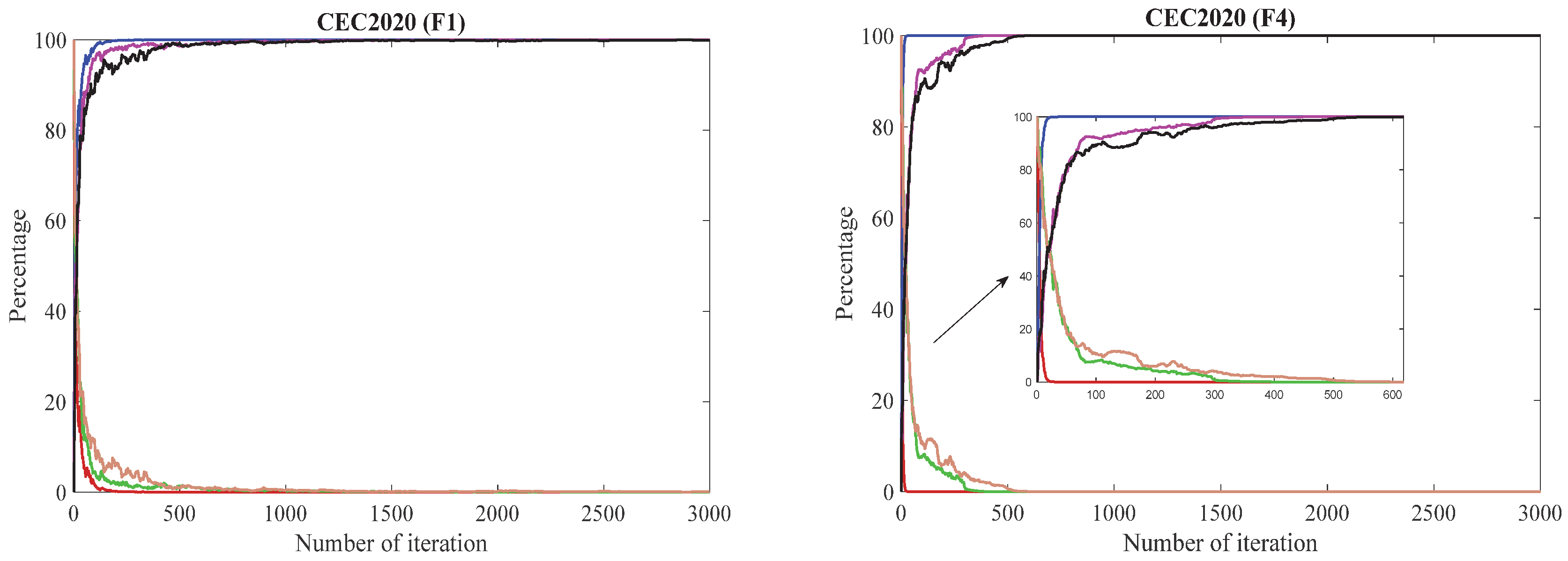
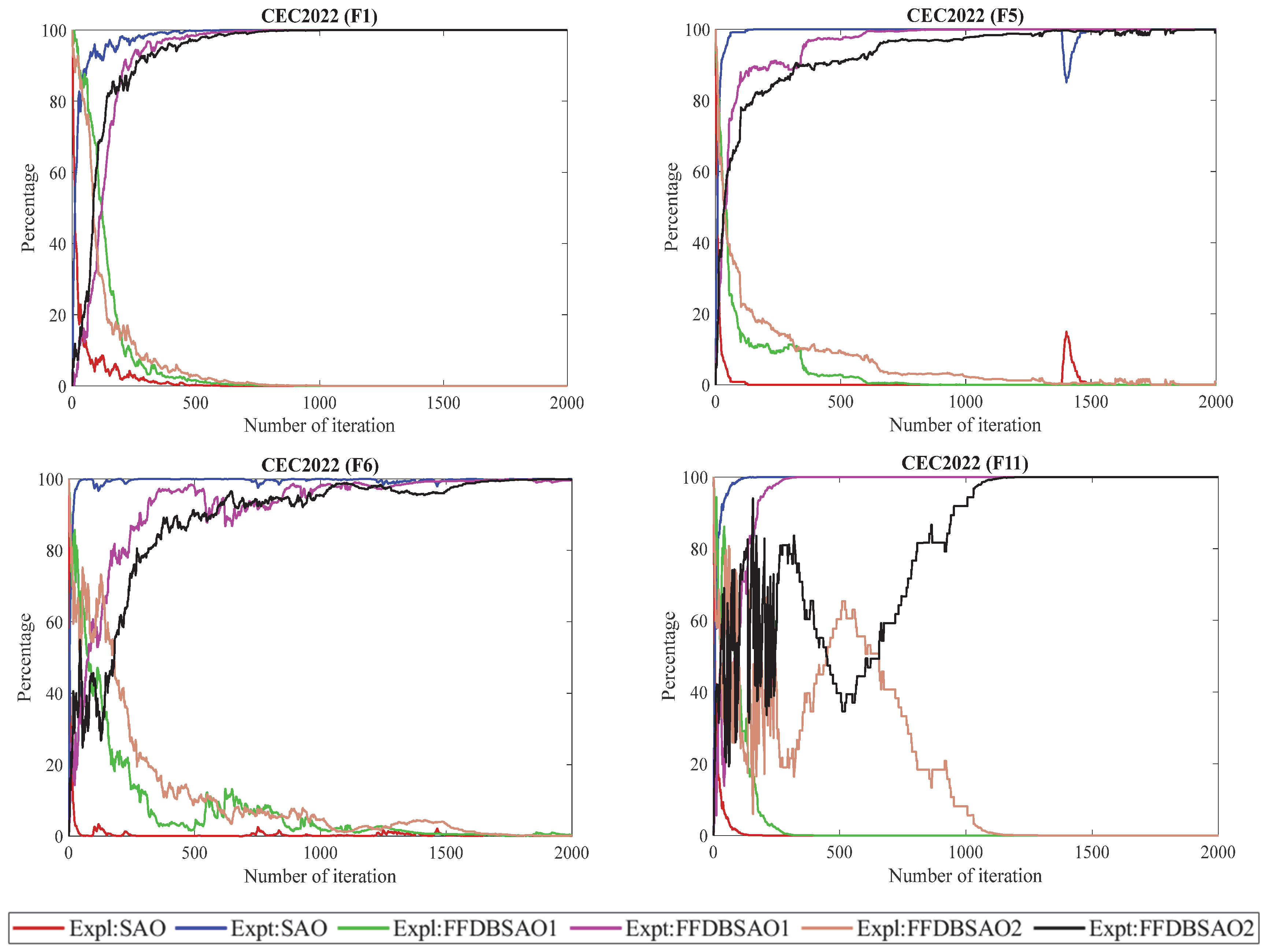
Figure 3 and
Figure 4 show the percentage change curves of the exploration and exploitation features of the SAO, FFDBSAO1, and FFDBSAO2 algorithms in each iteration during the solution of the optimization problem on the 30-dimensional CEC2020 and 20-dimensional CEC2022 benchmark functions. The figures demonstrate the investigation of the optimization algorithm behaviors during exploration and exploitation as they handle different problems in the CEC2020 and CEC2022 benchmark test functions. A meaningful comparison between basic SAO and the developed FFDBSAO1, along with FFDBSAO2, is made to evaluate their performance in reaching the optimal solution.
Among the CEC2020 and CEC2022 benchmark test functions, the F1 function is defined as a unimodal test function. In this type of function, the exploration process of the SAO algorithm ends quickly, while the exploitation process increases rapidly and exhibits unstable behavior in the phase of finding the optimal solution. The FFDBSAO1 and FFDBSAO2 algorithms started the optimization process with dynamic exploration behavior. The FFDBSAO2 algorithm took longer to solve the F1 function in both benchmark test suites than the FFDBSAO1 algorithm, which shows that the algorithm successfully performs the exploitation process without becoming stuck in local solution traps, unlike the other algorithms, when searching for the optimal solution.
Among the CEC2020 and CEC2022 benchmark test functions, the F4 and F5 functions are defined as basic test functions. For the F4 function in CEC2020, it is seen in
Figure 3 that the FFDBSAO2 algorithm exhibits a more balanced exploration and exploitation behavior than the SAO and FFDBSAO1 algorithms in searching for the optimal solution. For the F5 function in CEC2022, it is evident that the FFDBSAO2 algorithm exhibits the best exploration and exploitation behavior and is the algorithm with the least risk of early convergence without becoming stuck in local solution traps. While the SAO algorithm is the algorithm with the worst performance in solving this problem in terms of exploration and exploitation behaviors, it is seen in
Figure 4 that the FFDBSAO1 algorithm lags behind the FFDBSAO2 algorithm. However, it exhibits a balanced exploration and exploitation behavior.
Both the CEC2020 and CEC2022 benchmark suites include hybrid function types in their F7 and F6 solutions. The self-adjusting search approach of the FFDBSAO2 can be observed in
Figure 3, which depicts FFDBSAO2’s exploration and exploitation movements according to problem complexity during the solution search process. The algorithm demonstrates ongoing exploration behavior, which prevents it from becoming stuck in local suboptimal regions. The FFDBSAO2 algorithm operates with a minimized risk of reaching suboptimal results too early in the search process. The solution methods applied by the SAO and FFDBSAO1 match the FFDBSAO2 when dealing with this function, yet the algorithm’s exploration–exploitation equilibrium operates at a lower level than that of the FFDBSAO2. The optimization process of function F6, shown in
Figure 4, displayed dynamic balance between exploration and exploitation by the algorithms. At the beginning of the optimization process, the FFDBSAO2 emphasized exploration more than the other algorithms. The FFDBSAO2 algorithm began its solution search by investigating a wide range of search areas during the initial optimization period until it established its optimal search area. Over time, the longer gradual transition to the exploitation process compared to the SAO and FFDBSAO1 algorithms shows that the FFDBSAO2 algorithm successfully transitioned from the global search process to the local optimization process, allowing for the discovery of promising solutions.
The F10 and F11 functions in the CEC2020 and CEC2022 benchmark test suites are expressed as composition function types. For the F10 function, the FFDBSAO2 algorithm gradually transitions from exploration to exploitation in a balanced way. It is seen in
Figure 3 that the FFDBSAO2 algorithm continues to search for quality solutions around the optimal solution point after switching to the exploitation process and has a lower risk of early convergence compared to the SAO and FFDBSAO1 algorithms. For the F11 function, there are fluctuations in the exploration and exploitation characteristics of the FFDBSAO2 algorithm, which shows that the algorithm performs a balanced and powerful search to find the optimal solution. Thus, the FFDBSAO2 algorithm effectively improves solutions and exhibits convergence behavior towards optimum or near-optimum values. In solving this problem, although the FFDBSAO1 algorithm performs a balanced search in the exploration and exploitation process, it lags behind the FFDBSAO2 algorithm in terms of performance in finding the optimum solution. The SAO algorithm entered the early convergence process with weak exploration and exploitation behavior.
Usually, the success of optimization techniques depends on keeping a suitable balance between exploration and exploitation. A well-designed optimization algorithm guarantees that exploration is adequate to explore several areas of the solution space while switching to exploitation at the correct moment to expedite convergence.
Figure 3 and
Figure 4 underline the need for adaptive methods in optimization since various functions in the CEC2020 and CEC2022 benchmark test suites call for distinct exploration–exploitation strategies. The obtained results show that, by including more efficient exploration and exploitation characteristics than the SAO and FFDBSAO1 algorithms, the FFDBSAO2 method is more successful in converging to the optimal solution.
5.2. Application of the Proposed FFDBSAO Algorithm to the Economic Dispatch Problem
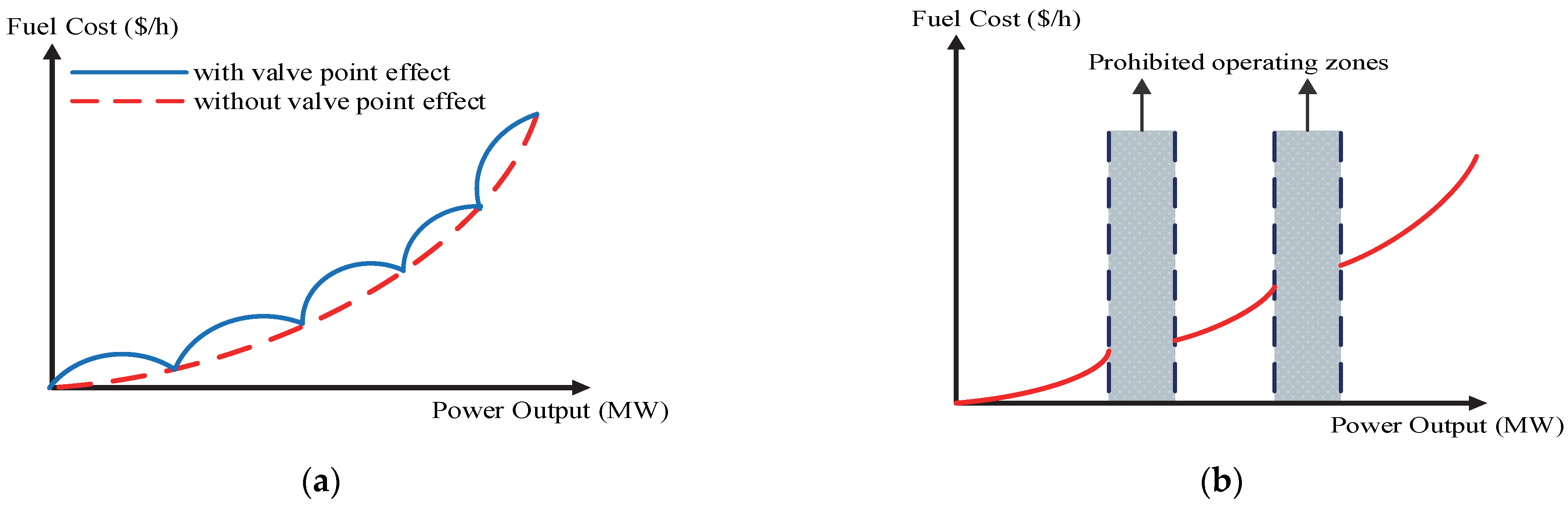
Variants of the FFDBSAO algorithm were used to try to solve the ED problem, which is one of the most important planning and operation problems in power systems, and a comparison of the results of the SAO algorithm with the results of existing algorithms in the literature is presented in this subsection. The results of the 11 best algorithms from the literature for each test case are presented in tables and discussed.
Table 6 shows the test systems used in solving the ED problem, the number of generators included in the test systems, the demand power of the systems, and the type of objective function to be minimized.
Test System 1: This includes six generators, where TL, RR, and POZs are considered. The system parameters are extracted from [
54].
Table S3 shows the values of the production units and total operating cost obtained as a result of the optimization process of SAO, as well as the proposed FFDBSAO1 and FFDBSAO2 algorithms. When the generator values of the FFDBSAO2 algorithm were substituted into the total fuel cost equation, it was computed as USD 15,444.1884/h. Also, when the generator values were substituted, they met the equality limits.
Table 7 presents the results of the 11 best algorithms from the literature and the results of the used SAO, FFDBSAO1, and FFDBSAO2 algorithms. The result of the proposed FFDBSAO2 approach was USD 5.4216/h, USD 5.6116/h, and USD 5.7016/h less than the results of the three best results in the literature, the RCBA, LM, and ST-IRDPSO algorithms, respectively.
Test Systems 2–3: Test systems 2 and 3 have ten generators and the total demand is 2700 MW. The difference between the two test systems is that VPE is not considered in test system 2, while VPE is considered in test system 3. The system parameters are extracted from [
55]. The results of the control variables obtained from the SAO, FFDBSAO1, and FFDBSAO2 algorithms as a result of the optimization process are given in
Table S4. The results of the SAO, FFDBSAO1, and FFDBSAO2 algorithms are presented in
Table 8, along with the best 12 results presented in the literature for both test systems. The FFDBSAO2 algorithm achieved the optimal value for both test systems when compared to the other algorithms in the literature. Moreover, for test system 2, the FFDBSAO2 algorithm met the equality bounds with an error value of 1 × 10
−4 when calculating the minimum fuel cost. For test system 3, it found the equality bound with an error value of zero and found the optimal solution value. This result proves that the algorithm effectively found the optimal solution.
Test System 4: This includes 13 generators, where only VPE is considered. The test system is evaluated at 1800 MW and 2520 MW conditions and at two different values of the coefficient to be used in the VPE of the third generator. The system parameters are taken from [
48]. Thus, simulation studies were carried out by considering test system 4 in four different ways.
Test system 4.1 shows the operating situation where the requested power is 1800 MW, and the coefficient value, including the VPE of the third generator, is taken as 200. The generator values obtained from FFDBSAO2 are given in detail in
Table S5. For test system 4.1,
Table 9 compares the results of the SAO, FFDBSAO1, and FFDBSAO2 algorithms with the results of the 13 best algorithms presented in the literature. The FFDBSAO2 algorithm stands out as the best algorithm from the literature comparison.
Test system 4.2 defines a system with the same generator fuel cost coefficients and a demanded power value of 2520 MW. The generator values obtained as a result of the simulation study carried out under these conditions are given in
Table S5. These generator values fulfilled the power balance equality constraint with a 1 × 10
−4 error value inside the predefined limit values. The comparison with the literature findings showed that SAO, FFDBSAO1, and FFDBSAO2 competed against the ten best algorithms from the literature-based studies on this test system. The FFDBSAO2 algorithm ranked third in achieving the optimal value, as shown in
Table S5.
In test system 4.3, the demanded power value is 1800 MW, and the third generator’s VPE coefficient value is 150.
Table S5 presents the results of the simulation studies carried out based on this system. According to the literature comparison, the FFDBSAO2 algorithm obtained a value USD 0.0061/h higher than the best result in the literature. These results prove that the FFDBSAO2 algorithm effectively converged to a value better than the best value in the literature.
In test system 4.4, the coefficient value of the VPE of the third generator remained the same as in test system 4.3, while the demanded power value was increased to 2520 MW. The results obtained from test system 4.4 are given in
Table S5. When the literature comparison in
Table 9 is examined, the FFDBSAO2 algorithm approaches the previous six best algorithms with an error value of 3.3107 × 10
−6%. This result shows that the FFDBSAO2 is a successful algorithm in finding the optimal result, similar to other algorithms in the literature.
Test System 5: This includes 13 generators, where TL and VPE are considered. While this test system met the demand power of 2520 MW, the third production unit was evaluated at two different values within the system’s cost coefficients. In addition, the coefficients in the loss matrix to calculate TL were considered in three ways. The test system was examined under four scenarios according to all these conditions. The test system parameters were taken from the relevant reference [
48].
For test system 5.1, a simulation study was conducted by accepting the demanded power of 2520 MW, and the cost coefficient of VPE of the third generator was 200. Here, the values of the production units optimized by the SAO, FFDBSAO1, and FFDBSAO2 algorithms are listed in
Table S6. A comparison with the literature is given in
Table 10. According to the comparison results, the FFDBSAO2 algorithm yielded the best value among the results of the other algorithms presented in the literature.
For test system 5.2, while all system data remain the same for test system 5.2, the coefficient value of −0.0017 for production unit no. 11 in the loss matrix is changed to 0.0017. The optimized generator values considering these system parameters are shown in
Table S6, and the literature comparison is listed in
Table 10. The comparison results show that FFDBSAO2 improved on the best value in the literature by USD 1.1429/h.
For test system 5.3, the values of two parameters in the loss matrix changed. The results of the FFDBSAO2 are presented in the fourth column of
Table S6. Moreover,
Table 10 shows that the total cost value obtained from the FFDBSAO2 was better than for the others presented in the literature comparison.
For test system 5.4, the VPE cost coefficient value of the third generator number was accepted as 150. The results from the simulation study are given in the fifth column of
Table S6. According to the comparison results in
Table 10, the FFDBSAO2 algorithm found USD 24,512.1812/h, improving on the best value in the literature by USD 0.2488/h.
Test System 6: This includes 15 generators, where the operational constraints are TL, RR, and POZs. Test system 6 is evaluated in two ways, and the system’s parameters are taken from [
48]. At the end of the optimization process, the values of the production units obtained by FFDBSAO2 are presented in
Table S7. For test system 6.1, when the optimized parameters were substituted into the fitness function and recalculated, it was seen that the FFDBSAO2 satisfied all inequality limits.
Table 11 shows the results of the 15 best algorithms in the literature. The FFDBSAO2 algorithm found the total production cost value as USD 32,692.3980/h, which was USD 8.812/h less than the result of the ESSA algorithm, the best result in the literature. For test system 6.2, simulation studies were conducted by changing the RR values of the second and fifth generators. The generator values obtained from FFDBSAO2 are shown in
Table S7. A comparison of the six best algorithms in the literature is presented in
Table 11. Accordingly, FFDBSAO2 showed a significant performance by finding a total fuel cost value of USD 6.6081/h less than the algorithm with the best value in the literature.
Test System 7: The system has 20 generation units, where only TL is considered. The system parameters are extracted from [
53]. The optimal production values obtained by the FFDBSAO2 algorithm are tabulated in
Table S8. The FFDBSAO2 provided the inequality limits when substituting these values into the fitness function. The results of the SAO, FFDBSAO1, and FFDBSAO2 algorithms are compared with those of the 13 best algorithms in the literature, which are presented in
Table 12. When examining
Table 12, the FFDBSAO2 algorithm obtained results closer to those of the algorithms listed before it, with an average of 3.36233 × 10
−6%.
Test System 8: The test system consists of 40 production units with eight-valve points. Here, three different scenarios were created by changing the fuel cost coefficients of the production units. The system parameters are obtained from [
48]. The optimal values of the production units obtained from the FFDBSAO2 for test systems 8.1, 8.2, and 8.3 are in
Table S9. Moreover, the literature comparison for these test systems is presented in
Table 13. According to these tables, for test system 8.1, the FFDBSAO2 algorithm showed remarkable success, finding a value close to the optimal result in the literature. For test system 8.2, the required power value and inequality limits were met when the optimal values in
Table S9 were returned to the system. According to the comparison results, the FFDBSAO2 achieved a value better than any presented in the literature. For test system 8.3, the comparison results presented in
Table 13 show that the FFDBSAO2 yielded the best value in the literature.
Test System 9: A large-scale power system with 110 generators is considered. The parameters of this system are taken from [
48]. The values of the production units obtained from the FFDBSAO2 are presented in
Table S10. A comparison of the total fuel cost values obtained from the SAO, FFDBSAO1, FFDBSAO2, and the results of nine algorithms presented in the literature is given in
Table 14. The FFDBSAO2 stands out as the algorithm closest to the best value presented by the HcSCA algorithm in the literature, with an error value of USD 0.0078/h. This result shows the solution’s quality and the proposed approach’s success.
5.2.1. Convergence and Statistical Analysis of the Optimization Algorithms for ED Problem
The SAO, FFDBSAO1, and FFDBSAO2 algorithms used for solving the ED problem were run 30 times for each test system. The statistical evaluation of the obtained results is presented in
Table S11. The minimum, mean, maximum, and standard deviation values presented in
Table S11 were examined, and the FFDBSAO2 algorithm achieved a significant superiority over the FFDBSAO1 and SAO algorithms. The results obtained from the simulation studies conducted for the operating conditions in each test system were evaluated using the non-parametric Wilcoxon signed-rank test. This test evaluates whether the median difference between the observations in paired samples is different from zero. In other words, it is a robust and versatile tool for comparing paired data for parametric tests. Two algorithms, named algorithm “C” and algorithm “D”, are used to perform this test. The application steps of this test are as follows.
Take the sum of the fitness values obtained during 30 independent runs of the two algorithms selected for comparison.
Calculate W+, the sum of simulation rankings for which algorithm C outperforms algorithm D in 30 independent runs.
Calculate W−, the sum of simulation rankings for which algorithm C performs worse than algorithm D in 30 independent runs.
The p-value is calculated to make the results obtained from this test more meaningful and to show their importance. If this value is smaller than the determined significance level, it is expressed as strong evidence against H0.
In other words, if the
p-value is smaller than the determined significance level value due to this test, the
H0 hypothesis is rejected, which means that the difference between the two measurements is significant. If it is larger than the significance level value, the
H0 hypothesis is accepted. In this study, the significance level is taken as
σ = 0.05. The results obtained from this test are given in
Table 15. A strong statistical trend emerged after examining the non-parametric statistical results obtained from 18 simulation studies. In many of the simulation studies, the FFDBSAO2 algorithm performed significantly better than the other algorithm, as expressed by the significant difference between
W+ and
W− and a very low
p-value. According to the results obtained from test system 1, the FFDBSAO2 outperformed the FFDBSAO1, as seen in a
W− value of 1 compared to
W+ of 464; the
p-value is 1.9209 × 10
−6, which led to the rejection of
H0. The pairwise rank test comparison of the FFDBSAO2 algorithm with SAO, with
W+ of 465 and
W− value of 0, indicates that the FFDBSAO2 performed much better than SAO. The
p-value is 1.7344 × 10
−6, which allows for the rejection of
H0. The results confirm that the FFDBSAO2 frequently outperformed the FFDBSAO1 and SAO. The downward trend in
p-values across the various test cases emphasizes the reliability of these findings. The statistically significant differences in most comparisons ensure that the observed performance changes are not due to random chance but reflect meaningful algorithmic improvements.
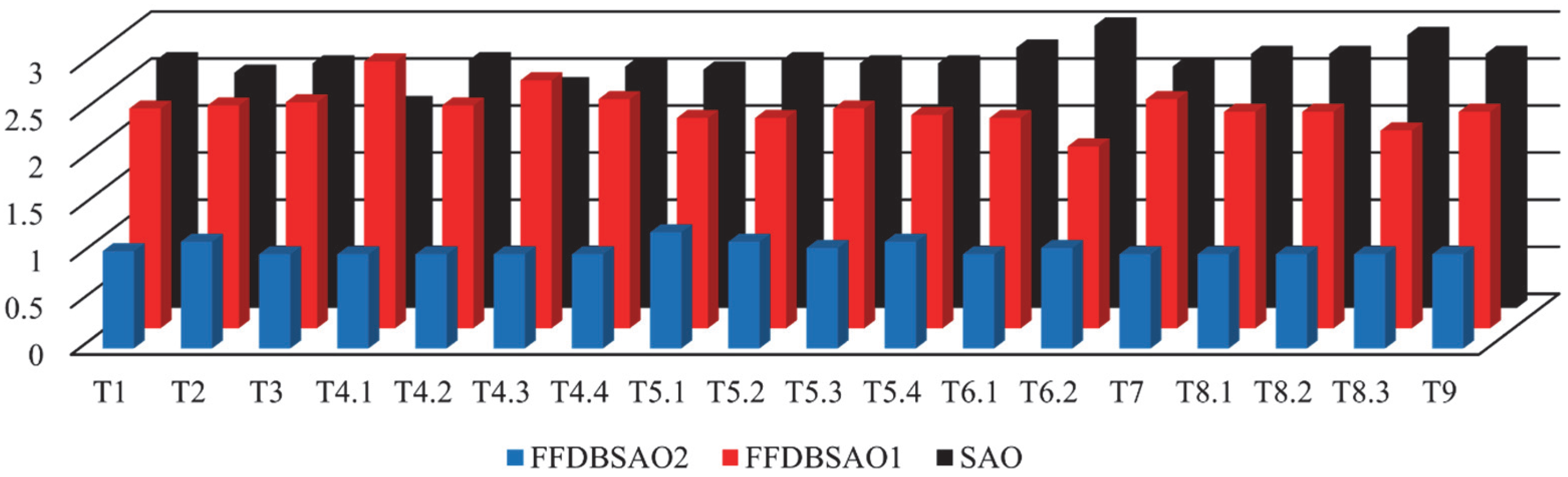
Moreover, the results obtained from the algorithms in 30 independent runs were subjected to a different statistical evaluation using Friedman analysis, one of the non-parametric statistical analysis methods. The Friedman scores obtained from 18 case studies are given in
Figure 5. When
Figure 5 is examined, it is seen that the Friedman scores of the FFDBSAO2 algorithm for each simulation run are overwhelmingly superior to the scores of the other algorithms.
Figure S12 presents the convergence graphs of the SAO, FFDBSAO1, and FFDBSAO2 for ED test cases. These graphs show how algorithm efficiency relates to operating cost development according to the fitness evaluation counts. All the test cases demonstrated that the FFDBSAO2 reached the optimal operating cost in the shortest possible time. The FFDBSAO2 achieved efficient cost reduction through its ability to complete its search within a restricted function evaluation range. Some test cases revealed that the SAO stopped progressing prematurely due to its inability to adjust the solution. The FFDBSAO1 algorithm exhibited a satisfactory performance level that exceeded SAO and came behind the superior FFDBSAO2. When the convergence graphs are examined in terms of final operating costs, the FFDBSAO2 algorithm showed strong optimization performance by reaching the lowest values among all the test cases. While the FFDBSAO1 reached competitive cost levels, it required significantly more fitness function evaluations to achieve this. On the other hand, the SAO struggled to reach a similar performance, as seen in test cases 5.4, 6.2, and 9, where it remained relatively stagnant. The effectiveness of the performances of these algorithms becomes more evident in different test cases; in lower-cost test cases such as test cases 2 and 3, all algorithms exhibited relatively close convergence trends, while the proposed FFDBSAO2 algorithm outperformed other algorithms in efficiency. In higher-cost test cases such as test cases 8.1 and 8.2, the FFDBSAO2 achieved a significantly lower operating cost in fewer evaluations, proving that its performance in convergence to the optimum point was better than the other algorithms. It is clear from
Figure S12 that despite the differences in problem complexity, the FFDBSAO2 algorithm consistently outperformed the other algorithms.
The performance on the ED problem shows visible links through box plots in
Figure S13 for SAO, FFDBSAO1, and FFDBSAO2 for all test cases.
Figure S13 expresses average operating cost distributions from multiple runs to show how changes in the fitness function affect stability during convergence, and the resilience of the methods. Consistent with a stable optimization performance, the FFDBSAO2 method routinely achieved the lowest median total cost in all test systems. The FFDBSAO2 algorithm demonstrated high stability as shown by its minimum interquartile range, indicating low result variability. Analysis of the plots indicates that the FFDBSAO consistently found high-quality solutions because extreme outliers do not appear in the data. The FFDBSAO2 boxplot shows compression at the low end during multiple test cases, thus enhancing solution quality by achieving optimal results with minimal deviation. The performance of the FFDBSAO1 stands between the SAO and FFDBSAO2 since it had lower costs than the SAO but did not equal the FFDBSAO2’s efficiency. However, the FFDBSAO1 showed a significant decreasing trend in the fitness function value, indicating that it improved over time, although it was not as efficient as FFDBSAO2. On the other hand, the SAO had the highest median value in almost all the test systems, as seen in
Figure S2. This made it the least efficient algorithm among the three algorithms.
5.2.2. Stability Analysis of the Optimization Algorithms for ED Problem
In this section, a stability analysis was applied to show the accuracy and reliability of the FFDBSAO2 algorithm in solving the ED problem compared to the FFDBSAO1 and SAO algorithms. Stability analysis is a method used in the literature to evaluate the performance of an algorithm in solving an optimization problem. It provides a comprehensive evaluation of the performance of an algorithm, measuring its efficiency, reliability, and computational cost [
51,
121].
It is beneficial for evaluating different algorithms and determining which is better for an optimization problem. While evaluating the performance of algorithms, three performance metrics, success rate, the average iteration number, and the average search time, are considered. The definitions of these metrics are given below.
Success rate (
SR, %): This is defined as the percentage of successful runs (
NSR) from the total runs (
NR) where the algorithm can obtain a feasible solution [
121]. For an optimization problem, a high
SR percentage indicates that the algorithm is a more accurate method, while a low
SR percentage indicates that the algorithm is not reliable. It is computed using Equation (29).
Average iteration number (
AIT): This can be defined as the average number of iterations for which the algorithm finds a feasible solution for multiple runs [
121]. Low iteration values mean the algorithm converges quickly to a feasible solution. The
AIT is calculated with Equation (30), where only the iteration numbers of the successful runs are considered in the calculation.
Average search time (
AST): The search time (st) is the duration required for an algorithm to obtain a feasible solution. The
AST is the average time of the algorithm’s successful runs across multiple runs [
121]. It is computed as
In this study, the eighteen ED case studies were considered and solved using the FFDBSAO2, FFDBSAO1, and SAO algorithms. The stability analysis results obtained from these algorithms are presented in
Table 16.
Assessment of SR values: According to
Table 16, among the three algorithms, the FFDBSAO2 established itself as the most proficient algorithm, with an 86.67% average
SR value, because it successfully generated solutions across all case studies. The high
SR value indicates that the FFDBSAO2 was the most dependable solution for these optimization problems. The average
SR values for the FFDBSAO1 and SAO were much lower, at 26.48% and 29.44%, respectively. The
SR values of the success rate for the FFDBSAO1 and SAO confirmed that their solutions were unreliable because no sufficient solutions were discovered in several iterations. The FFDBSAO2 demonstrated consistently high
SR values through individual test case observations because it found feasible solutions in all 100% of the examined case studies. Moreover, the FFDBSAO1 and SAO failed to discover feasible solutions since they recorded 0%
SR values in test systems 6.2, 8.1, 8.2, 8.3, and 9. Therefore, the FFDBSAO1 and SAO showed unreliable performance because their solutions remained inconsistent, making them unfit for stable practical optimization requirements.
Assessment of AST values: When evaluating
AST values, it is important to note that a lower MST is good only if
SR is high; otherwise, the algorithm finds solutions fast in rare cases but mostly fails. From
Table 16, the FFDBSAO1 and SAO had lower
AST values, with averages of 2.60 and 2.16 s, respectively, showing that they solved problems rapidly when they did succeed. However, because their
SR values were low, their speed advantage was less significant because they failed to solve most case studies. On the other hand, the FFDBSAO2, with an
AST of 9.59 s, took somewhat longer to converge but had a substantially better chance of success.
Assessment of AIT values: From
Table 16, the FFDBSAO2 was the most efficient in terms of iterations because it balanced feasibility and computational cost. The FFDBSAO1 and SAO took longer to converge, and since their
SR was low, this suggests that they often failed despite running many iterations. With an average of 940.27 iterations per successful run, FFDBSAO2 had the lowest
AIT value of the three algorithms. This proves that, in comparison to the other algorithms, FFDBSAO2 was computationally efficient since it needed fewer iterations to arrive at a workable solution. The SAO and FFDBSAO1 showed higher average
AIT values than the FFDBSAO2. With low success rates, the FFDBSAO1 and SAO’s higher MIT values indicate that they were unreliable and inefficient even when they succeeded.
Consequently, the FFDBSAO1 demonstrated better reliability, efficiency, and computational cost performance than FFDBSAO1 and SAO according to the stability analysis results. The FFDBSAO1 demonstrated the most reliable performance because it achieved an 86.67% SR value and operated with 940.27 iterations and a 9.59 s search time. The search times of the FFDBSAO1 and SAO were short, but their stability was compromised because of their inadequate success rates and excessive use of iterations. Practical implementations requiring dependable and steady performance should employ the FFDBSAO2 as the preferred algorithm.


 ,
, 


