Optimal Bidding Strategies for the Participation of Aggregators in Energy Flexibility Markets

Abstract

The increasing adoption of Renewable Energy Sources (RESs), due to international energy policies mainly related to the decarbonization of electricity production, raises several operating issues for power systems, which need “flexibility” in order to guarantee reliable and secure operation. RESs can be considered examples of Distributed Energy Resources (DERs), which are typically electric power generators connected to distribution networks, including photovoltaic and wind systems, fuel cells, micro-turbines, etc., as well as energy storage systems. In this case, improved operation of power systems can be achieved through coordinated control of groups of DERs by “aggregators”, who also offer a “flexibility service” to power systems that need to be appropriately remunerated according to market rules. The implementation of the aggregator function requires the development of tools to optimally operate, control, and dispatch the DERs to define their overall flexibility as a “market product” in the form of bids. The contribution of the present paper in this field is to propose a new optimization strategy for flexibility bidding to maximize the profit of the aggregator in flexibility markets. The proposed optimal scheduling procedure accounts for important practical and technical aspects related to the DERs’ operation and their flexibility estimation. A case study is also presented and discussed to demonstrate the validity of the method; the results clearly highlight the efficacy of the proposed approach, showing a profit increase of 10% in comparison with the base case without the use of the proposed methodology. It is evident that quantitatively more significant results can be obtained when larger aggregations (more participants) are considered.

1. Introduction

In recent decades, interest in and scientific research on climate change has significantly increased in EU countries. The main objective is to promote low carbon emissions and renewable energy-based technology diffusion to enable the decarbonization process, mainly in electricity production, distribution, and consumption.

The main set of goals established by the EU to be reached by the year 2030 include bringing the yearly electricity consumption covered by renewables to 30% and cutting greenhouse gas emissions by 55%. In this context, the concept of “electrification of everything” (e.g., heating and cooling systems, transportation, services inside buildings, etc.) has also arisen to obtain cleaner and more efficient power systems [1]. In the expected highly electricity-based economy, with a significant share of RESs and minimum use of gas to produce power, as well as energy, new system challenges pose many issues to the optimization of the power system and the RESs’ operation while properly adapting the electricity market design [2]. During the energy transition, the distribution networks in particular will have to deal with important critical operating conditions since the distribution network is the natural “platform” where the different energy stakeholders and technologies will have to interact and integrate with each other [3].

In the past, the planning approach adopted by the most important DSOs was the “fit-and-forget” method, which consists of grid planning by considering the worst-case scenarios, when foreseeable [3]. Given an expected expansion in the electrification of consumption, this approach would result in excessive investments to upgrade the distribution networks [2]. On the other hand, the SG paradigm is gradually providing new control solutions to cope with challenging operation issues in the modern power system. Accordingly, electricity supply must also provide ASs, such as balancing/flexibility services delivered to ensure reliable system operations. The opening of the ASM to new flexible users (e.g., RESs and storage systems) will be of primary importance to support the grid during the upcoming years of transition. It is planned that millions of energy and flexibility service providers, hybrid vehicles, and storage facilities will be able to provide energy and flexibility in the European electricity market by 2030 [4].

The flexibility services, intended as tools to meet “grid needs”, can also be useful for the DSO to help avoid/defer excessive network investments in the coming years [5]. Moreover, “power flexibility” can be used not only to provide technical services to cope with distribution grid congestion issues [6] or to increase the grid hosting capacity [7] but also to help improve the efficiency of electricity markets [8].

According to this framework, the aggregator can be defined as a player who can buy and sell power flexibility (provided by aggregated entities/sources) in dedicated markets; therefore, they collect, control, and manage a portfolio of DERs to maximize their value for the energy infrastructure [3].

Several works have focused on the energy management system of aggregators that use flexibility to provide ASs to the TSO/DSO while providing economic benefits to the end-users. The aggregator needs optimization tools to define market products in the form of bids. The bidding problem related to the aggregators’ activity in the markets has been widely investigated in the literature. Several researchers have investigated the issue of “aggregation optimization”. A critical review on the role of “energy management system aggregators” was provided in [9], considering the SG context and the participation of different resources in the provision of ASs. The participation of an aggregator in the energy market has been proposed in some papers, exploiting an MILP procedure, as in [10,11,12,13,14]; in particular, ref. [10] adopts a bilevel MILP problem. All of the mentioned papers optimized domestic loads, storage, and generation systems which helped the users to reduce energy costs. The optimal management of consumers’ flexibility for the bidding strategies of an aggregator in the day-ahead market was addressed in [14] in order to maximize the aggregator’s payoff. In [15], the authors propose a scalable optimization scheme designed for prosumers providing ancillary services; prosumers were modeled using MILPs, enabling the authors to consider different operating modes. Paper [16] addresses the participation of aggregators of thermostatically controlled loads in electricity markets, using a stochastic optimization model to define demand bids for the day-ahead energy market; the authors modeled weather and load uncertainties through a set of scenarios.

Paper [17] proposes a method for designing network-aware flexibility requests for distribution-level flexibility markets. It employs an optimization model with chance constraints and a LinDistFlow approximation to capture both physical grid constraints and uncertainty from renewables or load fluctuations. Ref. [18] introduces an MILP formulation for aggregating flexible consumers, considering both economic operation and dispatch modes to evaluate potential revenue and meet committed flexibility services. Paper [19] proposes an approximate dynamic programming (ADP) framework for aggregating flexibility and cost, leveraging computational geometry tools to design efficient numerical schemes and avoid solving multiple OPF problems. Finally, in [20], the authors investigate the impact of reward and market timeframes on flexibility and aggregator profit; the amount of flexibility and the aggregation profit depend on the time-differentiated prices and the incentives.

All the above-mentioned papers have proposed optimization methods to define bids through the optimization of one or more types of flexible resources. Furthermore, all works do not consider distribution network constraints in the optimization models. They assume that the DSO must be capable of solving all the possible network problems that may arise because of the bidding strategies.

On the contrary, another group of papers addresses the network problem by proposing a set of network-constrained bidding optimization models. These bidding models define energy and reserve bids constrained by the technical limits of the distribution networks. For instance, ref. [20] proposes stochastic models to compute energy bids through the optimization of electrical and/or thermal energy storage units. These bidding models use linear equations to constrain network power injections. Nonetheless, these constraints do not ensure the network feasibility of the aggregators’ bids because they do not provide any observability over line power flows and voltages. Instead, in [21,22], an efficient grid congestion management power flow algorithm with flexible assets is proposed. Papers [17,23] formulate an algorithm capable of providing flexibility to DSOs, and [24] presents a bilevel agent-based optimization algorithm including the DSO operation cost. The approach suggested in [25] assumes that the DSO quantifies the flexibility needed to solve the grid problem, suggesting that operating costs are a separate problem and the aggregator just assists them.

Finally, it is important to remark that while the present paper is devoted to bidding optimization, many works are focused on ensuring the optimal sizing of the aggregator’s portfolio. For example, in [26,27], a profitable and flexible DER recruitment–participation approach is proposed.

With reference to the reviewed literature, some issues can be highlighted in the majority of the proposed optimization algorithms, including the following:

• They deal with the aggregation’s trading issues only, without including the flexibility service in the optimization process;
• They neglect important parameters accounting for technical aspects and constraints of resources’ operation (e.g., response time);
• They do not consider the need for flexibility in the aggregators’ estimation, in terms of both quantity and price, to make appropriate offers to the market.

Starting from the above considerations, the present paper aims to contribute to the field of large-scale aggregator portfolio (defined as a set of PTAs) optimal scheduling by proposing a new flexibility bidding optimization strategy that maximizes the aggregators’ profits in the energy flexibility market, intending to provide bid offers to the FMs. In particular, the focus of the paper is on the formulation of a centrally managed and implemented optimization problem for an aggregate energy flexibility service provision from different DERs in which flexibility estimation is introduced by considering technical constraints on DER operation.

The paper is structured as follows. Section 2 presents the role of the aggregator, according to the business model assumed in the present paper. The approach for the proposed “optimal bidding strategy” is described in detail in Section 3. Finally, the simulation results are presented and discussed with reference to a case study in Section 4.

2. The Role of the Aggregator in Flexibility Markets

In Europe, thanks to a regulatory process driven by EU institutions, most countries currently have electricity markets with structures that are very similar to each other. The aggregator can be represented as an intermediary between the customers, grouped into clusters, and the wholesale markets.

The proposed FM model is a day-ahead market for ancillary services in which the participants (high-power customers and/or aggregators) offer a given amount of flexibility in relation to price for the subsequent 24 h. The FM for the given time horizon is executed after the closure of the energy market, once the generation and consumption of the participants are defined. The adopted model is a flexibility exchange platform in a specific geographical area, based on a “pay-as-bid” approach; in practice, the flexibility is traded as energy.

In [28,29], the USEF Flexibility Value Chain provides an overview of the sixteen types of flexibility services which can be offered to all markets and products through distributed flexibility, according to different purposes. In the present paper, “constraint management services” are considered, which will help the grid operators (TSOs and DSOs) to optimize grid operation using physical constraints made available to them through the markets.

Considering the FM model adopted in this study, the aggregator’s tasks are summarized as follows:

• The aggregator engages different types of active and passive customers by signing contracts based on their typical load profiles and features to gather flexibility.
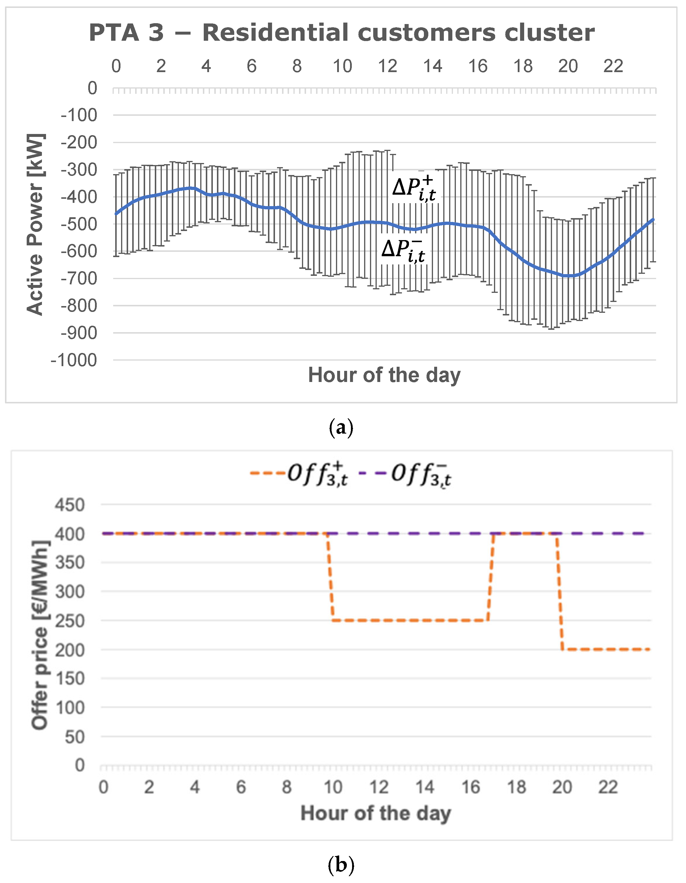
• For each fixed time interval, the customers offer flexibility in terms of a couple of values representing “quantity and price”, where “quantity” can be identified by an active power variation for a given time interval, associated with a “price” (monetary reward). It is important to remark that the feasibility of the different customers’ offers/availability is not under the aggregator’s responsibility. In other words, the feasibility check of the proposed active power variations provided by the customers is only the task of some of them, considering the types of loads, generators, and storage available to the customers.
• From the FM viewpoint, the aggregator sells the available cluster power variations obtained thanks to the flexibility provided by the customers by offering price–quantity bids. The profits are shared between the aggregator and the customers, according to a “profit-seeking” approach.

The problem is, then, to find an optimal bidding strategy that maximizes the expected aggregator profit, based on optimal management of the flexibility offered by the customers’ cluster. The formulation of the bidding problem is a challenging task, since complex interactions occur among the various types of resources, and a variety of uncertainties, including the behavior of variable and discontinuous DERs, need to be considered.

From this perspective, the aggregator has two responsibilities:

• Before the market closure, they have to decide the optimal price–quantity bids to be sent to the market for all the periods within the trading horizon, according to the offers/availability of the PTAs;
• They must decide the optimal schedules for every flexible unit (i.e., PTA) in their portfolio.

Figure 1 describes the timeline that can be assumed for the two aforementioned tasks, where D indicates the dispatching day and D-1 is the previous day.

The present paper deals with Point 1, which involves the definition of the bidding optimization strategy. This task, referred to as “Bids calculation” (Figure 1), is performed in a time interval between 24 h and 2–3 h before the start of the trading horizon (note that the typical size of the trading horizon is equal to one day), when the aggregator knows the availability of the PTAs. The results of the market can be communicated to the PTAs according to a transparency policy in the aggregation. The second task, referred to as “Schedule decision” (Figure 1), which is out of scope for the present paper, regards the definition of the optimal set point of all the resources starting from a defined quantity requested by the TSO/DSO. In fact, this quantity will be known only if the offers of the aggregator are accepted. Typically, the aggregators’ bids in the market may, or may not, be activated, depending on the TSO/DSO activations and market clearing results.

The proposed used methodology and the steps involved in conducting the present research study can be summarized with the flowchart reported in Figure 2. In particular, the following steps are included:

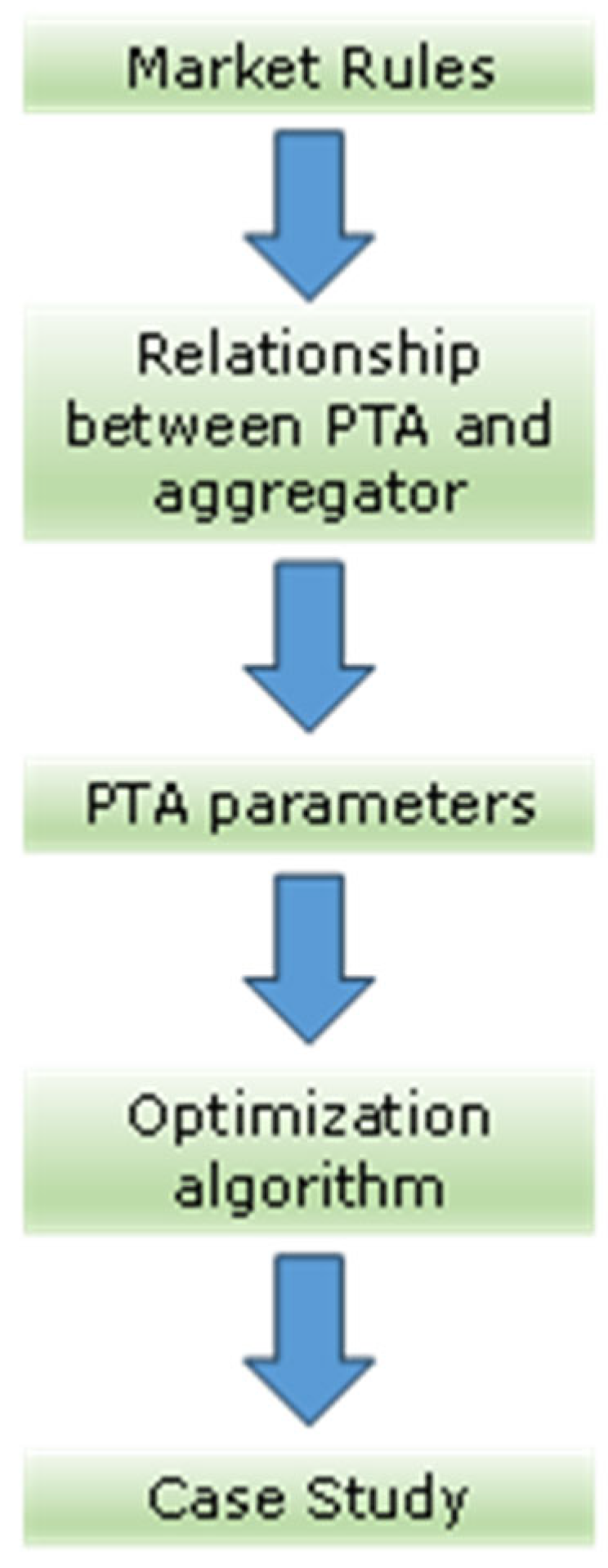
• Definition of market rules to establish the rules governing how the aggregate can operate in the FM.
• Definition of the relationship between PTAs and aggregator; this is useful to define how PTAs can contribute to the aggregation in a profitable way for all the stakeholders.
• Definition of main PTA parameters; this is useful to specify the features and metrics of the PTAs.
• Definition of a suitable optimization algorithm; an algorithm can be created to optimize the performance of the aggregate, as will be described in the next section.
• Case study and numerical analysis, with the aim of analyzing the effectiveness of the implementation, performing quantitative assessments to validate the results.

3. Optimal Bidding Strategy: Mathematical Formulation

This section describes the mathematical formulation of the bidding strategy approach proposed in the present paper.

The main task of the proposed optimization algorithm is the definition of the bidding strategy in all the time intervals of the adopted trading horizon. In particular, the methodology is useful to define the quantity of electric power and the price that can be offered by the aggregator in the FM.

The inputs of the optimization procedure are as follows:

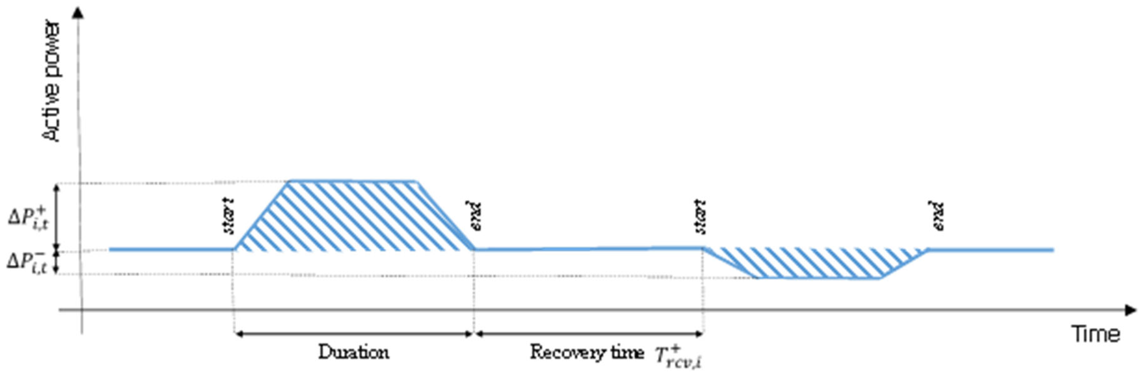
• The availability of a single PTA included in the aggregator’s portfolio, defined by the maximum power variation available in all the time intervals, in terms of power increase or decrease (Figure 3);
• Maximum/minimum duration and recovery time of the power variations (Figure 3) for all the PTAs;
• Fixed cost and bid price submitted by all PTAs to the aggregator;
• FM price (estimated value) considered for the aggregate power increase or decrease;
• Aggregate power minimum variation and minimum duration (market constraints on the aggregation).

The optimization is performed with the aim of maximizing the difference between the DER’s costs and the aggregator’s revenue obtained in the FM, considering some technical limits and constraints regarding the single PTA and/or the market technical rules.

To obtain the mathematical formulation, that is a nonlinear optimization problem, the following items will be defined:

• Variables (integer and real).
• Optimization function.
• Constraints, which can be divided into “time constraints” and “market constraints”.

The typical formulation for the proposed approach is presented in (1), where the different matrices can be used to define the linear constraints in a suitable way; similarly, the nonlinear constraints are expressed by the function c(x,z):

$$\underset{x,z}{\max }OF such that\left\{\begin{array}{c}LB\le x\le UB\\ A·x\le b\\ c\left(x,z\right)\le 0\end{array}\right.$$

(1)

3.1. Physical Variables (Active Powers)

The problem variables that form vector x are the power variations in the i-th PTA in time t, indicated as ${∆P}_i^t$. A PTA can be a single customer, a DER, an MG, or an LEC included in the aggregator’s portfolio. The variation is referred to the “expected profile” (called “baseline” in the paper), which can be derived from a load forecast analysis performed by the aggregator and/or by each PTA. Such variables must be limited by bounds (2), contained within matrices UB and LB in (1):

$${{∆P}_{i,t}^{-}\le ∆P}_i^t\le {∆P}_{i,t}^{+} {\forall i\in N}_{PTA},\forall t\in T$$

(2)

where N_PTA is the number of participants in the aggregation and ${∆P}_i^t$ is the power variations in a PTA, as defined above, contained in vector x. The bid of the aggregator is obtained by summing the power variations in all the PTAs.

3.2. Status Variables

The status variables, which form vector z in the canonical formulation expressed by (1), are used to indicate the PTAs’ operating status in terms of the “starting and ending time of power output variation”. They are useful for defining some constraints regarding the PTAs’ operation schedule, such as the nonlinear constraints indicated in (1). In particular, the following status variables can be defined as follows:

• “Start PTA up status” (active power increase), ${\delta }_{start,i,t}^{up}$, which relates to time t, when the i-th PTA starts its power increase, as defined in (3):

  $${\delta }_{start,i,t}^{up}=\left\{\begin{array}{c}1 if \left(\left({∆P}_i^{t-1}\le 0\right) or\left(t=1\right)\right) and \left({∆P}_i^t>0\right) \\ 0 otherwise\end{array}\right.$$

  (3)
• “Start PTA down status” (active power decrease), ${\delta }_{start,i,t}^{dn}$, which relates to time t, when the i-th PTA starts its power decrease, as defined in (4):

  $${\delta }_{start,i,t}^{dn}=\left\{\begin{array}{c}1 if \left(\left({∆P}_i^{t-1}\ge 0\right) or\left(t=1\right)\right) and \left({∆P}_i^t<0\right) \\ 0 otherwise\end{array}\right.$$

  (4)
• “End PTA up status” (active power increase), ${\delta }_{end,i,t}^{up}$, which relates to time t, when the i-th PTA ends its power increase, as defined in (5):

  $${\delta }_{end,i,t}^{up}=\left\{\begin{array}{c}1 if \left({∆P}_i^{t-1}>0\right) and \left({∆P}_i^t\le 0\right) \\ 0 otherwise or \left(t=1\right)\end{array}\right.$$

  (5)
• “End PTA down status” (active power decrease), ${\delta }_{end,i,t}^{dn}$, which relates to time t, when the i-th PTA ends its power decrease, as defined in (6):

  $${\delta }_{end,i,t}^{dn}=\left\{\begin{array}{c}1 if \left({∆P}_i^{t-1}\le 0\right) and \left({∆P}_i^t>0\right) \\ 0 otherwise.or.\left(t=1\right)\end{array}\right.$$

  (6)

3.3. Cost Functions

The cost functions are adopted to estimate the cost for the aggregator to reward the PTAs for their contribution to the aggregate flexibility.

The expected cost can be formulated by means of two terms:

• A fixed cost, which includes the amount that cannot be related to each PTA power variation;
• A variable cost, which regards the power variation offered by each PTA.

According to this classification, the fixed cost for the i-th PTA can be formulated as follows:

$$C_i^{fix}=C_{on,i}^{+}·{\sum }_{i=1}^{N_{int}}{\delta }_{start,i,t}^{up}+C_{on,i}^{-}·{\sum }_{i=1}^{N_{int}}{\delta }_{start,i,t}^{dn}$$

(7)

The variable cost, which depends on the power variation requested to each PTA, is formulated in (8):

$$C_{i,t}^{var}\left({∆P}_i^t\right)=\left\{\begin{array}{c}{Off}_{i,t}^{+}·{∆P}_i^t·∆t if {∆P}_i^t\ge 0\\ {Off}_{i,t}^{-}·\left|{∆P}_i^t\right|·∆t if {∆P}_i^t<0\end{array}\right.$$

(8)

As discussed above, the aggregator rewards the PTAs for their contribution to the aggregate power flexibility. On the other hand, the aggregator makes a profit by selling flexibility to the FM. Therefore, the expected revenue for the aggregator, R_t, can be indicated as follows:

$$R_t\left({∆P}_i^t\right)=\left\{\begin{array}{c}{Price}_t^{+}·∆t·\sum _{i=1}^{N_{PTA}}{∆P}_i^t if\sum _{i=1}^{N_{PTA}}{∆P}_i^t\ge 0\\ {Price}_t^{-}·∆t·\sum _{i=1}^{N_{PTA}}\left|{∆P}_i^t\right| if\sum _{i=1}^{N_{PTA}}{∆P}_i^t<0\end{array}\right.$$

(9)

Costs and revenues are defined as their expected values since they would only be actual values when the offers proposed by the aggregator are accepted in the FM.

3.4. Objective Function

The OF needs a formulation suitable to maximize the difference between the revenues and the costs for the aggregator.

Consequently, the total expected aggregator’s revenue, R_tot, can be written as follows:

$$R_{tot}={\sum }_{t=1}^{N_{int}}{R}_t\left({∆P}_i^t\right)$$

(10)

The total cost, C_tot, is calculated as follows:

$$C_{tot}={\sum }_{i=1}^{N_{PTA}}{\sum }_{t=1}^{N_{int}}{C}_{i,t}^{var}\left({∆P}_i^t\right)+{\sum }_{i=1}^{N_{PTA}}{C}_i^{fix}$$

(11)

Finally, the OF is defined in (12) and represents the profit of the aggregator:

$$\mathrm{O}\mathrm{F}=R_{tot}-C_{tot}$$

(12)

3.5. Constraints

The optimization constraints can be divided into “time constraints” and “market constraints”.

The first category mainly regards the following time parameters, defined for each PTA:

• Maximum duration of the PTA power variation;
• Minimum duration of the PTA power variation;
• Recovery time, i.e., the time interval between two subsequent power variations.

To satisfy the time constraints, other equations need to be included in the model, following the formulation proposed in [30].

The maximum duration constraint, expressed by using the status variables described in Equations (3)–(6), is shown in (13) and (14) for power increase and decrease, respectively:

$${\sum }_{j=t}^{t+D_{max,i}^{+}-1}{\delta }_{end,i,j}^{up}\ge {\delta }_{start,i,t}^{up}\hspace{1em}\forall t\in T$$

(13)

$${\sum }_{j=t}^{t+D_{max,i}^{-}-1}{\delta }_{end,i,j}^{dn}\ge {\delta }_{start,i,t}^{dn}\hspace{1em}\forall t\in T$$

(14)

Similarly, the minimum duration constraint is shown in (15) and (16) for power increase and decrease, respectively:

$${\delta }_{start,i,t}^{up}+{\sum }_{j=t}^{t+D_{min,i}^{+}-2}{\delta }_{end,i,j}^{up}\le 1\hspace{1em}\forall t\in T$$

(15)

$${\begin{array}{c} \\ \delta \end{array}}_{start,i,t}^{dn}+{\sum }_{j=t}^{t+D_{min,i}^{-}-2}{\delta }_{end,i,j}^{dn}\le 1\hspace{1em}\forall t\in T$$

(16)

The constraint on the recovery time is obtained by adding to the mathematical models, as shown in Equations (17) and (18):

$${\delta }_{end,i,t}^{up}+{\sum }_{j=t}^{t+T_{rcv,i}^{+}}{\delta }_{start,i,j}^{up}\le 1\hspace{1em}\forall t\in T$$

(17)

$${\delta }_{end,i,t}^{dn}+{\sum }_{j=t}^{t+T_{rcv,i}^{-}}{\delta }_{start,i,j}^{dn}\le 1\hspace{1em}\forall t\in T$$

(18)

The recovery time constraint is applied only to variations in the same direction; this assumption refers to the different PTAs’ behavior to satisfy the power variation requested.

The market constraints mainly regard the aggregate power minimum variation limit and the related minimum duration.

The minimum duration of the aggregate power variation can be obtained by adding the constraint expressed by (19):

$${\sum }_{i=1}^{N_{PTA}}{∆P}_i^t\le {\sum }_{i=1}^{N_{PTA}}{∆P}_i^{t+1}\le \cdots \le {\sum }_{i=1}^{N_{PTA}}{∆P}_i^{t+T_m}\hspace{1em}\forall t\in T$$

(19)

The limit value aggregate power minimum variation is normally different for the two requested flexibility services, i.e., power variation “increase” or “decrease”. The related constraint conditions that can be added to the model are shown in (20a) and (20b), respectively. At each optimization run, only one of the constraint conditions will be adopted, as described in the next section.

$${\sum }_{i=1}^{N_{PTA}}{∆P}_i^t\ge P_{min}^{+}\hspace{1em}\forall t\in T$$

(20a)

$${\sum }_{i=1}^{N_{PTA}}{∆P}_i^t\le {-P}_{min}^{-}\hspace{1em}\forall t\in T$$

(20b)

The adoption of this type of constraints depends on the adopted market rules. However, in the proposed approach, these constraints have been included without loss of generality; in fact, should other market models not include this type of operational condition, the constraints could be disregarded by using suitable values for T_m, $P_{min}^{+},$ and $P_{min}^{-}$ in the optimization procedure.

3.6. Procedure’s Output

The expected output of the proposed method is the power variation (offer size—OS) that the aggregator can submit to the FM. The OS at time t is obtained by adding all the optimal power variations in all PTAs, as formulated in (21):

$$OS\left(t\right)={\sum }_{i=1}^{N_{PTA}}{∆P}_i^t\hspace{1em}\forall t\in T$$

(21)

Finally, a couple of quantities, offer size (OS) and price (Price) for each time interval, will form the aggregator’s bid in the FM.

The proposed approach can lead to an “increase power mode” or a “decrease power mode”. In fact, it is possible to run the optimization algorithm in the following ways:

(a)

Run in the “increase power mode”, considering constraints 20a;

(b)

Run in the “decrease power mode”, considering constraints 20b;

According to these “run modes”, different outputs of the proposed procedure can be obtained in order to enable the possibility of providing multiple bids to the FM. However, it is important to remark that, according to the system requirements, only one type of power variation (increase/decrease) will be accepted in the FM, based on the DSO/TSO needs.

4. Results and Discussion Related to a Case Study

In this section, the developed case study is presented to demonstrate the validity of the proposed method; the first subsection is devoted to the case study description, while the second one regards the results presentation. The optimization problem, described in Section 3, has been implemented and solved by using a numerical model developed in the MATLAB^® (9.13.0.2553342 (R2022b) Update 9) environment [31]; in particular, the SQP, which represents the state of the art in nonlinear programming methods [32], has been used to solve the proposed optimization problem.

4.1. Case Study

The present case study includes the participation of three PTAs:

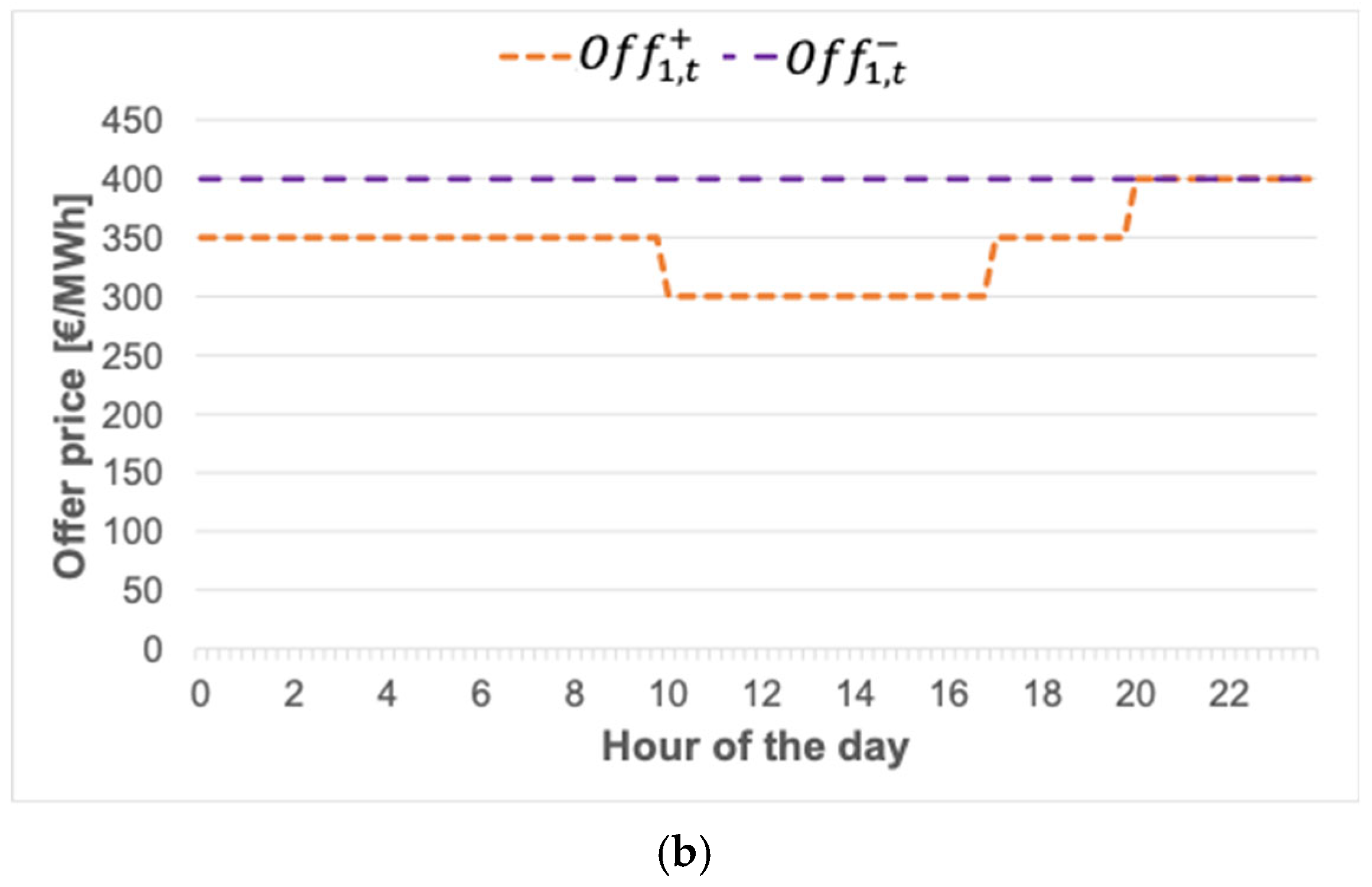
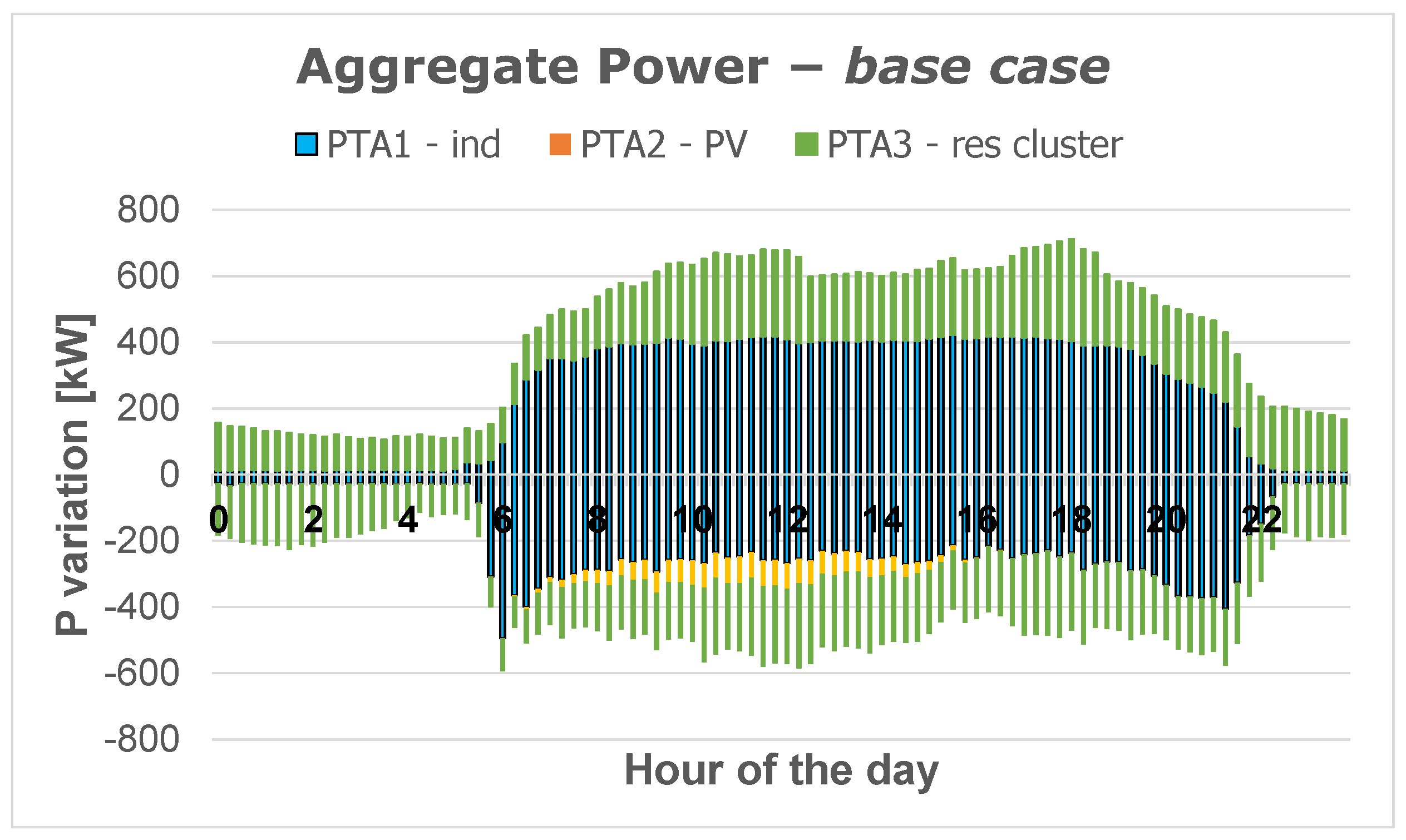
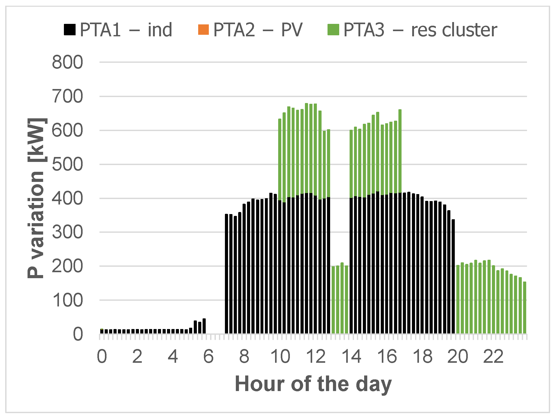
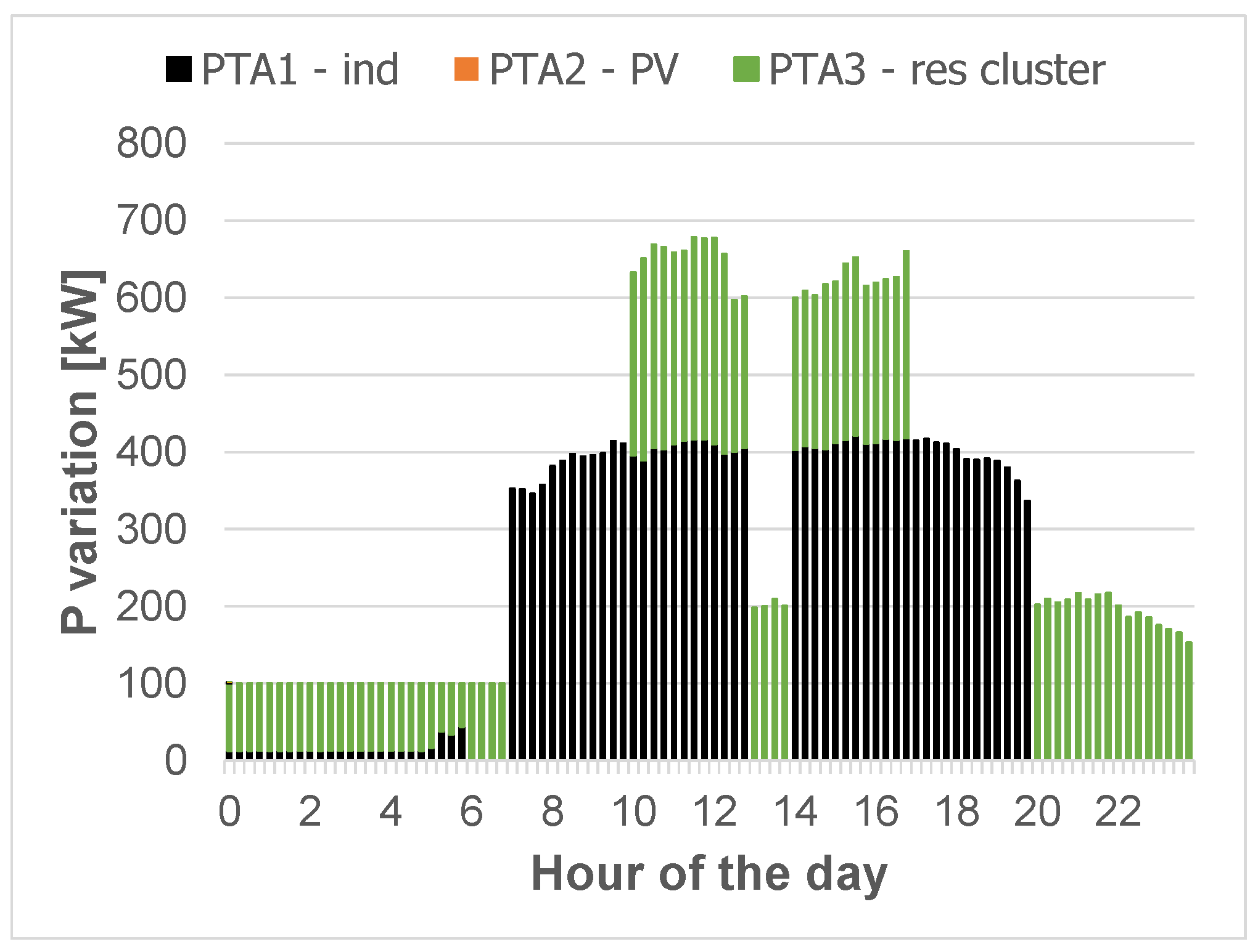
• PTA 1, represented by an industrial load.
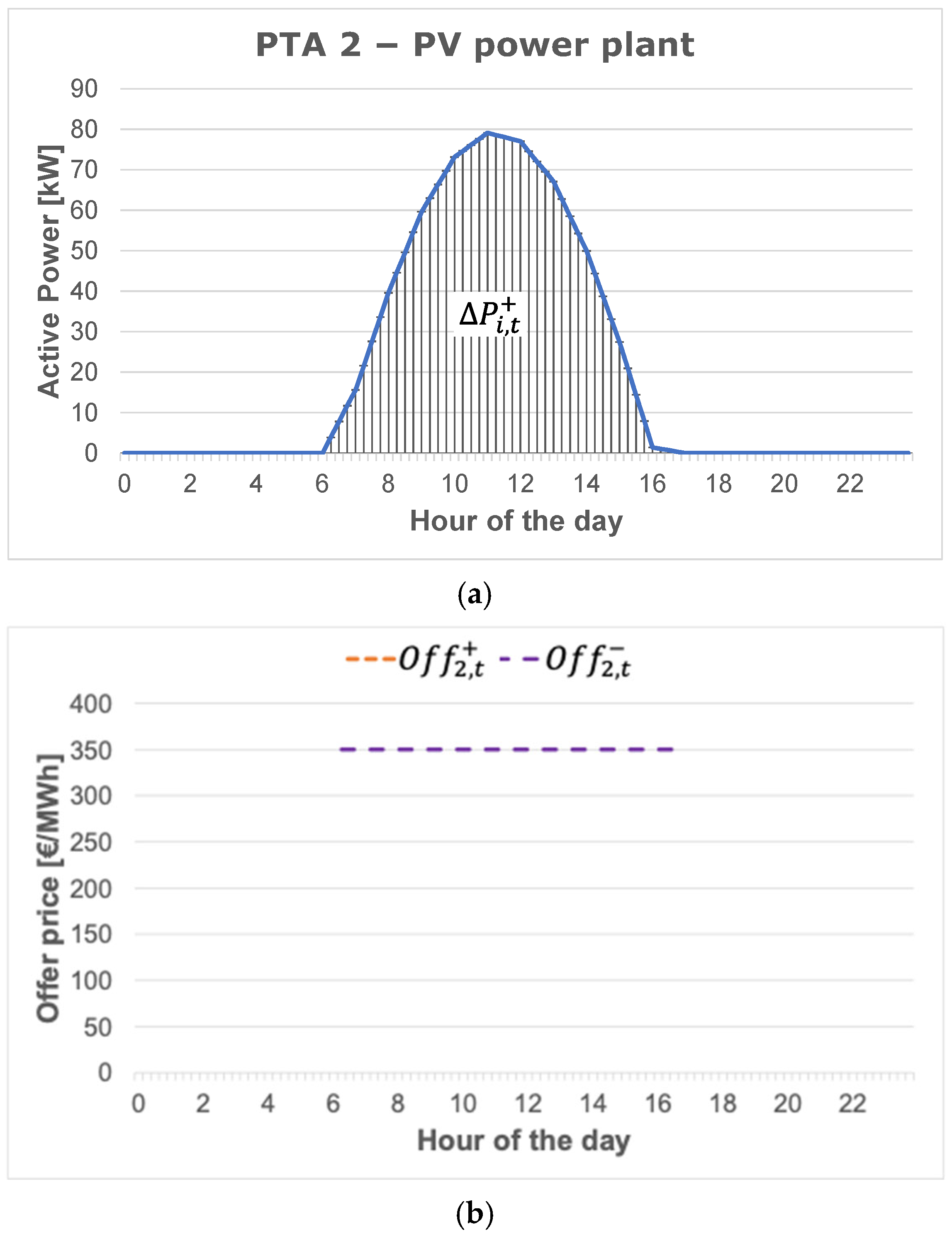
• PTA 2, including a PV generator.
• PTA 3, including a cluster of 1,135 residential customers. These customers have been clustered according to their similar characteristics in terms of “availability” and “prices” offered to the aggregator.

Then, the considered case study includes the participation of three different PTAs only in order to simplify the presentation of the results without affecting the generality of the proposed approach. The three PTAs, as well as their aggregation, act as an equivalent generator from the viewpoint of the external network. This means that a positive power variation (upward bid) in the PTAs results in increased power generation that can also be obtained by a reduction in the PTAs’ power consumption. Similarly, a negative power variation (downward bid) means an increased withdrawn power from the external network, i.e., an increased net consumption of the PTAs.

The main parameters for the PTAs ($D_{max,i}^{+}$, $D_{max,i}^{-}$, $D_{min,i}^{+}$, $D_{min,i}^{-}$, $T_{rcv,i}^{+}$ and $T_{rcv,i}^{-}$) included in the case study are shown in

Table 1. Main parameters of the PTAs included in the case study.

PTA Type	${\mathit{C}}_{\mathit{i}}^{\mathit{f}\mathit{i}\mathit{x}}$	${\mathit{D}}_{\mathit{m}\mathit{a}\mathit{x},\mathit{i}}^{+}$	${\mathit{D}}_{\mathit{m}\mathit{a}\mathit{x},\mathit{i}}^{-}$	${\mathit{D}}_{\mathit{m}\mathit{i}\mathit{n},\mathit{i}}^{+}$	${\mathit{D}}_{\mathit{m}\mathit{i}\mathit{n},\mathit{i}}^{-}$	${\mathit{T}}_{\mathit{r}\mathit{c}\mathit{v},\mathit{i}}^{+}$	${\mathit{T}}_{\mathit{r}\mathit{c}\mathit{v},\mathit{i}}^{-}$
1—Industrial load	0	6 h	6 h	15 min	15 min	1	1
2—PV generator	0	∞	∞	15 min	15 min	0	0
3—Cluster of residential customers	0	∞	∞	15 min	15 min	0	0

. In the table, the symbol “∞” identifies an infinite value for the parameters; in other words, the parameter (in this case the maximum variation duration) to which this value is associated does not affect the optimization. In fact, PTA2 and PTA3 (i.e., the PV generator and the cluster of residential customers) present a high level of flexibility: no “time constraint” is associated with them. On the other hand, PTA1 (i.e., the industrial load) is less flexible, with a maximum variation duration, $D_{max}$, equal to 6 h for both types of power variations (“increase” and “decrease”); the associated recovery time is equal to 1 h (Table 1).

The trading horizon is one day (24 h) with a time step of 15 min (Δt = 0.25 h; N_int = 96); the “baseline profiles” and the prices are referred to a single day of the year (a winter weekday). The fixed costs, $C_i^{fix}$, for all the PTAs are neglected for the sake of simplicity. The simplicity of the case study allows us to clearly present the results. All the PTA parameters adopted for the case study are based on realistic data coming from non-public practical cases, while the parameters related to the PTAs’ participation availability are elaborated based on realistic assumptions.

Figure 4a illustrates the time-dependent parameters of PTA1 (industrial load), i.e., maximum power variation available at time t, in terms of both power increase or decrease (positive or negative variation), with reference to the baseline for the selected day (the values in the baseline profile are negative since the PTA is a “load”). The dotted lines in Figure 4b identify the bid prices submitted by the PTA to the aggregator (${Off}_{1,t}^{+}$ and ${Off}_{1,t}^{-}$) for the upward and downward variations, respectively.

Similarly, the profiles of PTA2 and PTA3 in terms of maximum active power variations and bid prices are shown in Figure 5 and Figure 6, respectively; the PV generator does not offer any active power variation in upward mode.

The FM price is not known at the time the optimization problem is solved. Consequently, the proposed approach needs to exploit some statistical analysis performed on the FM historical data to obtain different FM daily price profiles that can be used for defining the aggregator’s bid. Various techniques can be used to perform a statistical analysis, but, in general, different FM price profiles can be obtained according to the profitability levels. The statistical analysis can, for example, return the following results:

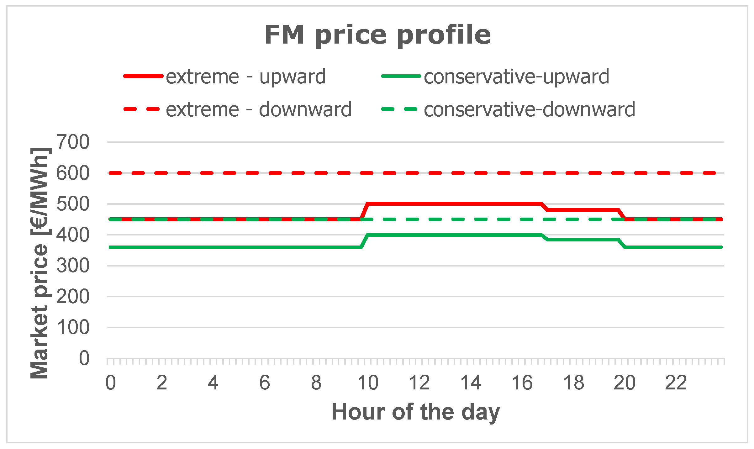
• An “average” FM price profile referred to the average clearing price in the FM during a given time period (e.g., one month/year);
• An “extreme” (“conservative”) FM price profile, calculated with reference to the “maximum” (“minimum”) clearing price in the FM during the same period.

The calculation of different FM price profiles is required to analyze multiple scenarios in terms of combinations of FM price profiles with different run modes, as discussed in Section 3.6, to obtain different bids according to the proposed methodology.

Finally, the FM price profiles assumed in the case study are reported in Figure 7. In particular, two specific price profiles are adopted (the “extreme” and the “conservative” one, thus defining an extreme and a conservative scenario accordingly). The strategy used in defining bid prices is based on realistic assumptions since statistic values deriving from participation in FM do not exist, neither in the literature nor in practice.

4.2. Results

In the “non-optimized case”, starting from each PTA’s power availability in the trading horizon, a base case is obtained, summing up all the active power variations, as indicated in Figure 8, in which different colors are used to highlight the contribution of the three PTAs. The aggregate power variation, both upward and downward, will correspond to different bids. The expected aggregator’s cost and profit in the simulated trading horizon (one day) in the two FM “price scenarios” are indicated in

Table 2. Cost and revenue for the aggregator in the trading horizon (base case).

		FM Price Scenarios
		Extreme	Conservative
	Aggregator Cost (to the PTAs) ${\mathit{C}}_{\mathit{t}\mathit{o}\mathit{t}}$	Aggregator Profit ${\mathit{O}\mathit{F}}_{\mathit{o}\mathit{p}\mathit{t}}$
base case—upward	EUR 3.3 k	EUR 1.6 k	EUR 0.6 k
base case—downward	EUR 3.8 k	EUR 1.9 k	EUR 0.5 k

. The aggregator’s profit is of EUR 1.6 k for the simulated trading horizon in the “extreme” FM price scenario. In fact, in the same period and for the same FM price scenario, the aggregator pays EUR 3.3 k to the PTAs for the requested power variations in upward mode and earns EUR 4.9 k in the FM for the aggregate power variation offered (supposed to be actually supplied to the network). Similar comments can be made for the downward mode.

In the “optimized case”, the proposed algorithm is run in multiple modes by using the FM price profiles shown in Figure 7, while the mathematical model presented in (1) has been used in both “increase power mode” (upward variation) and “decrease power mode” (downward variation) (see Section 3.6 for details). The aggregator’s profits obtained thanks to the proposed PTAs optimal scheduling are EUR 1.5 k (

Table 3. Profits of the aggregator in the trading horizon (optimized case).

	FM Price Scenario
	Extreme	Conservative
	$\mathbf{Aggregator} \mathbf{Profit} {\mathit{O}\mathit{F}}_{\mathit{o}\mathit{p}\mathit{t}}$
optimization case—upward	EUR 1.5 k (−7.4%)	EUR 0.7 k (+6.5%) EUR 0.6 k (+2.6%) [Pmin = 100 kW]
optimization case—downward	EUR 1.7 k (−10.3%)	EUR 0.5 k (−10.0%)

) for the simulated trading horizon (one day) in the “extreme” FM price scenario; compared with the base case, the profit is reduced but, in this case, the “time constraint” for the PTAs (maximum duration and recovery time for the PTA 1) is satisfied. In the same case, the “conservative” scenario has also been simulated; in the aggregate power variation, shown in Figure 9, it is apparent that in some intervals, the aggregate power variation is null, because the lower value in the FM prices makes it unprofitable to offer aggregate power considering the PTA’s offers (Figure 3, Figure 4 and Figure 5). The adoption of the proposed bidding strategy allows the aggregator to obtain a profit of EUR 0.7 k in the trading horizon (+6.5% with respect to the base case, adopted as reference).

Alternative PTA profiles can be formulated without performing any optimization, but it becomes difficult to satisfy the time constraints for each PTA and to obtain a revenue comparable with the aforementioned one, especially in the presence of a high number of PTAs.

The proposed aggregated power variation profile shown in Figure 9 highlights that in this case, no minimum power is guaranteed to participate in the FM in all time intervals. The use of this “market constraint” (see Section 3.5 for details) is, however, of particular importance in the real world because this is normally present in the common market rules which the aggregators must comply with. It is worth noting that the adoption of this constraint is one of the contributions of this work to the state of the art. Then, the results of another simulation that includes an aggregate power minimum variation limit (equal to 100 kW) are shown in Figure 10. In this “constrained case”, the daily trading aggregate power variation bid submitted to the FM market has been modified to satisfy the considered global constraint; compared to the “unconstrained case”, the profit decreases, but it is important to remark that the constraint is mandatory for the aggregator to participate in the FM. Consequently, such a result is more realistic.

Similar comments could be made for the optimization procedure performed in “decrease power mode” (downward variation). For this reason, the downward profiles have not been shown; however, it is important to remark that in the downward variation, the PV generator would be involved too in the aggregate power variation bid.

5. Conclusions and Future Developments

The paper aims to contribute to the field of large-scale aggregator portfolio (defined as the set of PTAs) optimal scheduling.

The current state of the art can be summarized as follows:

• The main aggregation trading issues do not include the flexibility service in the optimization process;
• Important parameters accounting for technical aspects and constraints of resources’ operation (e.g., response time) are neglected.

Starting from the above considerations, the present paper proposes an innovative method to optimize the flexibility bidding of aggregators who need to maximize their profits in future flexibility markets. In particular, the focus of the paper is on the formulation of a centrally managed and implemented optimization problem for an aggregate energy flexibility service provision from different DERs in which the flexibility estimation is introduced by considering technical constraints on the DERs’ operation.

The discussed case study demonstrates the effectiveness of the proposed procedure, which uses time constraints usually not included in the formulations available in the literature. The considered case study, which includes the participation of only three different but representative PTAs, has been proposed to simplify the presentation of the results, without affecting the generality of the proposed approach. Increasing the number of PTAs cannot provide additional information, while, on the contrary, the description of the inputs, the presentation, and the result understanding can be improved in comparison with alternative case studies that involve many PTAs. The lower power for the PV generator in comparison with the other PTAs does not influence the validity of the approach because this can influence the profits for the aggregator in terms of absolute value only.

Additionally, it is important to highlight that the scope of the proposed approach is the bidding optimization for a prefixed set of PTAs (aggregator’s portfolio), while portfolio optimization can be obtained with suitable methodologies that are out of scope for the present paper.

The results show how optimal PTA scheduling can enhance the aggregator’s profit; even in the intentionally simple case study proposed, the profit increase can be estimated to be 10% in comparison with a “base case” without any optimization. It is evident that more remarkable results would be obtained in scenarios with a higher number of aggregated PTAs. In that case, the proposed procedure would allow us to address a more complex optimization problem, since the latter would be unfeasible without a strategic constrained scheduling tool.

Finally, performing a study in the presence of multiple competing aggregators for the same ancillary services market represents an interesting task for future research. Moreover, a challenging aspect would be the definition of the “optimal set point” for all the involved PTAs obtained from the power variations requested by the TSO and/or DSO.

References

1. Silva, N. Tracing the transition from Passive to Active Distribution Networks. 2017. Available online: https://www.incite-itn.eu/blog/tracing-the-transition-from-passive-to-active-distribution-networks/ (accessed on 18 May 2025).
2. Tina, G.M.; Cavalieri, S.; Soma, G.G.; Viano, G.; De Fiore, S.; Grillo, P.; Distefano, L. Main features of an aggregator’s platform for the management of distributed energy resources—PASCAL project case study. In Proceedings of the 2020 AEIT International Annual Conference (AEIT), Catania, Italy, 23–25 September 2020; pp. 1–6. [Google Scholar]
3. Minniti, S.; Haque, N.; Nguyen, P.; Pemen, G. Pemen, Energies, Local markets for flexibility trading: Key stages and enablers. Energies 2018, 11, 3074. [Google Scholar] [CrossRef]
4. Celli, G.; Pilo, F.; Pisano, G.; Ruggeri, S.; Soma, G.G. Risk-oriented planning for flexibility-based distribution system development. Sustain. Energy Grids Netw. 2022, 30, 100594. [Google Scholar] [CrossRef]
5. Beckstedde, E.; Meeus, L. From ‘fit and forget’ to ‘flex or regret’ in distribution grids: Dealing with congestion in European distribution grids. IEEE Power Energy Mag. 2023, 21, 45–52. [Google Scholar] [CrossRef]
6. Celli, G.; Pisano, G.; Ruggeri, S.; Soma, G.G.; Pilo, F.; Papa, C.; Pregagnoli, C.; de Carolis, L.; Ferrero, S.; Cazzato, F. Distribution Systems as Catalysts for Energy Transition Embedding Flexibility in Large-Scale Applications. IEEE Access 2024, 12, 92227–92240. [Google Scholar] [CrossRef]
7. Eid, C.; Codani, P.; Perez, Y.; Reneses, J.; Hakvoort, R. Managing electric flexibility from distributed energy resources: A review of incentives for market design. Renew. Sustain. Energy Rev. 2016, 64, 237–247. [Google Scholar] [CrossRef]
8. Carreiro, A.M.; Jorge, H.M.; Antunes, C.H. Energy management systems aggregators: A literature survey. Renew. Sustain. Energy Rev. 2017, 73, 1160–1172. [Google Scholar] [CrossRef]
9. Asimakopoulou, G.E.; Hatziargyriou, N.D. Evaluation of economic benefits of DER aggregation. IEEE Trans. Sustain. Energy 2017, 9, 499–510. [Google Scholar] [CrossRef]
10. Nizami, M.S.H.; Hossain, M.J.; Mahmud, K.; Ravishankar, J. Energy cost optimization and DER scheduling for unified energy management system of residential neighbourhood. In Proceedings of the 2018 IEEE International Conference on Environment and Electrical Engineering and 2018 IEEE Industrial and Commercial Power Systems Europe (EEEIC / I&CPS Europe), Palermo, Italy, 12–15 June 2018; pp. 1–6. [Google Scholar]
11. Nizami, M.S.H.; Hossain, M.J.; Amin, B.M.R.; Kashif, M.; Fernandez, E.; Mahmud, K. Transactive energy trading of residential prosumers using battery energy storage systems. In Proceedings of the IEEE PowerTech2019, Milan, Italy, 23–27 June 2019; pp. 1–6. [Google Scholar]
12. Hatziargyriou, N.; Asimakopoulou, G.E. DER integration through a monopoly DER aggregator. Energy Policy 2020, 137, 111124. [Google Scholar] [CrossRef]
13. Parvania, M.; Fotuhi-Firuzabad, M.; Shahidehpour, M. Optimal demand response aggregation in wholesale electricity markets. IEEE Trans. Smart Grid 2013, 4, 1957–1965. [Google Scholar] [CrossRef]
14. La Bella, A.; Falsone, A.; Ioli, D.; Prandini, M.; Scattolini, R. A mixed-integer distributed approach to prosumers aggregation for providing balancing services. Int. J. Electr. Power Energy Syst. 2021, 133, 107228. [Google Scholar] [CrossRef]
15. Chen, S.; Chen, Q.; Xu, Y. Strategic bidding and compensation mechanism for a load aggregator with direct thermostat control capabilities. IEEE Trans. Smart Grid 2018, 9, 2327–2336. [Google Scholar] [CrossRef]
16. Prat, E.; Dukovska, I.; Herre, L.; Nellikkath, R.; Thoma, M.; Chatzivasileiadis, S. Network-Aware Flexibility Requests for Distribution-Level Flexibility Markets. IEEE Trans. Power Syst. 2024, 39, 2641–2652. [Google Scholar] [CrossRef]
17. Dib, M.; Abdallah, R.; Dib, O. Optimization Approach for the Aggregation of Flexible Consumers. Electronics 2022, 11, 628. [Google Scholar] [CrossRef]
18. Bandeira, M.B.; Faulwasser, T.; Engelmann, A. An ADP framework for flexibility and cost aggregation: Guarantees and open problems. Electr. Power Syst. Res. 2024, 234, 110818. [Google Scholar] [CrossRef]
19. Rasouli, V.; Gomes, Á.; Antunes, C.H. An optimization model to characterize the aggregated flexibility responsiveness of residential end-users. Int. J. Electr. Power Energy Syst. 2023, 144, 108563. [Google Scholar] [CrossRef]
20. Good, N.; Mancarella, P. Flexibility in multi-energy communities with electrical and thermal storage: A stochastic, robust approach for multi-service demand response. IEEE Trans. Smart Grid 2019, 10, 503–513. [Google Scholar] [CrossRef]
21. Dietrich, K.; Latorre, L.M.; Olmos, L.; Ramos, A. Modelling and assessing the impacts of self-supply and market-revenue driven Virtual Power Plants. Electr. Power Syst. Res. 2015, 119, 462–470. [Google Scholar] [CrossRef]
22. Jin, X.; Wu, Q.; Jia, H. Local flexibility markets: Literature review on concepts, models and clearing methods. Appl. Energy 2020, 261, 114387. [Google Scholar] [CrossRef]
23. Alrumayh, O.; Bhattacharya, K. Flexibility of residential loads for demand response provisions in smart grid. IEEE Trans. Smart Grid 2019, 10, 6284–6297. [Google Scholar] [CrossRef]
24. Hu, S.; Xiang, Y.; Liu, J.; Gu, C.; Zhang, X.; Tian, Y.; Liu, Z.; Xiong, J. Agent-based coordinated operation strategy for active distribution network with distributed energy resources. IEEE Trans. Ind. Appl. 2019, 55, 3310–3320. [Google Scholar] [CrossRef]
25. Lu, X.; Qiu, J.; Zhang, C.; Lei, G.; Zhu, J. Seizing unconventional arbitrage opportunities in virtual power plants: A profitable and flexible recruitment approach. Appl. Energy 2024, 358, 122628. [Google Scholar] [CrossRef]
26. Lu, X.; Qiu, J.; Zhang, C.; Lei, G.; Zhu, J. Assembly and Competition for Virtual Power Plants With Multiple ESPs Through a “Recruitment-Participation” Approach. IEEE Trans. Power Syst. 2024, 39, 4382–4396. [Google Scholar] [CrossRef]
27. Zoeller, H.; Reischboeck, M.; Henselmeyer, S. Managing volatility in distribution networks with active network management. In Proceedings of the CIRED Workshop, Helsinki, Finland, 4–15 June 2016; pp. 1–4. [Google Scholar]
28. USEF. White Paper: Flexibility Deployment in Europe; USEF: Lexington, KY, USA, 2021. [Google Scholar]
29. USEF. Position Paper Flexibility Value Chain; USEF: Lexington, KY, USA, 2018. [Google Scholar]
30. Ottesen, S.Ø.; Tomasgard, A.; Fleten, S.E. Multi market bidding strategies for demand side flexibility aggregators in electricity markets. Energy 2018, 149, 120–134. [Google Scholar] [CrossRef]
31. Mathworks, “Optimization toolbox User’s Guide”; MathWorks: Natick, MA, USA, 2022.
32. Boggs, P.T.; Tolle, J.W. Sequential Quadratic Programming for Large-Scale Nonlinear Optimization. J. Comput. Appl. Math. 2000, 124, 123–137. [Google Scholar] [CrossRef]
Figure 1. Timeline for the aggregator’s tasks in the flexibility market.
Energies 18 02870 g001
Figure 2. Flowchart of the proposed research study.
Energies 18 02870 g002
Figure 3. Definition of the parameters of the i-th PTA in the aggregation.
Energies 18 02870 g003
Figure 4. (a) PTA1 profiles: maximum active power variations. (b) PTA1 profiles: bid prices.
Energies 18 02870 g004aEnergies 18 02870 g004b
Figure 5. PTA2 profiles: maximum active power variations (a) and bid prices (b).
Energies 18 02870 g005
Figure 6. (a) PTA3 profiles: maximum active power variations. (b) PTA3 profiles: bid prices.
Energies 18 02870 g006
Figure 7. FM price profiles adopted by the algorithm for the case study.
Energies 18 02870 g007
Figure 8. Non-optimized aggregate power given by the sum of the PTAs’ power profiles (base case).
Energies 18 02870 g008
Figure 9. Optimized aggregate power—sum of the PTAs’ power profiles (“conservative” scenario).
Energies 18 02870 g009
Figure 10. Optimized aggregate power given by the sum of the PTAs’ power profiles (“conservative” scenario), under the minimum variation constraint (100 kW).
Energies 18 02870 g010