Coordinated Reactive Power–Voltage Control in Distribution Networks with High-Penetration Photovoltaic Systems Using Adaptive Feature Mode Decomposition

Abstract

As the proportion of renewable energy continues to increase, the large-scale grid integration of photovoltaic (PV) generation presents new technical challenges for reactive power balance in power systems. This paper proposes a coordinated reactive power and voltage optimization method based on Filtered Multiband Decomposition (FMD). First, to address the stochastic fluctuations of PV power, an improved FMD-based prediction model is developed. The model employs an adaptive finite impulse response (FIR) filter to decompose signals and captures periodicity and uncertainty through kurtosis-based feature extraction. By utilizing adaptive function windows for multiband signal decomposition, combined with kernel principal component analysis (KPCA) for dimensionality reduction and a long short-term memory (LSTM) network for prediction, the model significantly enhances forecasting accuracy. Second, to tackle the challenges of integrating high-penetration distributed PV while maintaining reactive power balance, a multi-head attention-based velocity update strategy is introduced within a multi-objective particle swarm optimization (MOPSO) framework. This strategy quantifies the spatial distance and fitness differences of historical best solutions, constructing a dynamic weight allocation mechanism to adaptively adjust particle search direction and step size. Finally, the effectiveness of the proposed method is validated through an improved IEEE 33-bus test case.

1. Introduction

With the increasing consumption of fossil fuels, renewable energy sources have gained significant attention. Among them, PV generation has rapidly emerged as a research hotspot due to its low cost and environmental benefits [1,2,3,4]. However, the large-scale integration of high-penetration PV generation poses substantial challenges to power system operation. In particular, the stochastic and intermittent nature of PV output has profound impacts on voltage stability, reactive power balance, and network losses [5,6,7,8].

Accurate PV power forecasting plays a crucial role in enhancing grid stability, optimizing reactive power distribution in distribution networks, and improving power system dispatch efficiency [9,10,11]. To address the challenges posed by PV output uncertainty—such as voltage stability issues and reactive power imbalance—improving PV forecasting accuracy and optimizing reactive power distribution in distribution networks have become active research areas. Traditional neural network models for PV forecasting [12,13,14] are often constrained by the availability of power plant data and tend to overlook the influence of certain environmental factors on PV output [15]. Additionally, conventional networks exhibit inherent limitations in handling long-term dependencies, feature analysis, and variable-length output generation, while also being highly dependent on meticulous hyperparameter tuning. PV power output is influenced by multiple factors, exhibiting complex nonlinear relationships with various environmental features, making precise modeling challenging. To accelerate model convergence, researchers have developed numerous optimization algorithms [16,17,18]. However, slower convergence rates can lead to overfitting issues, limiting the general applicability of existing models under diverse operating conditions. Moreover, most existing approaches fail to adequately consider the time-varying characteristics of PV power, restricting improvements in forecasting accuracy. In response to these challenges, hybrid forecasting models have emerged, combining physical modeling with data-driven techniques to leverage the strengths of multiple technologies, thereby significantly improving forecasting accuracy and system reliability. For instance, Ref. [19] proposes a hybrid model that integrates empirical mode decomposition (EMD), principal component analysis (PCA), and LSTM networks based on the methodology in Ref. [20]. This model demonstrates superior performance in terms of spectral occupancy variation and effectively improves forecasting accuracy. Further research in Ref. [21] demonstrated that global horizontal irradiance (GHI) is a key environmental factor influencing PV power generation, and that hybrid forecasting models outperform single models in terms of prediction accuracy.

On the basis of accurately forecasting distributed PV output, the rational coordination of reactive power distribution in high-penetration PV distribution networks can enhance grid operation efficiency, reduce energy consumption and losses, and provide technical support for integrating renewable energy into distribution networks. Reactive power optimization is a critical aspect of optimal power flow (OPF) in power systems and requires efficient optimization algorithms for its solution [22,23,24,25]. In recent years, artificial intelligence and machine learning algorithms have been widely applied to reactive power optimization, including Grey Wolf Optimization (GWO), Genetic Algorithm (GA), Multi-Objective Particle Swarm Optimization (MOPSO), and Whale Optimization Algorithm (WOA). However, these algorithms are prone to local optima, which affects their practical application. To address this issue, researchers have proposed various improvements. Ref. [26] introduced a reactive power optimization method for distribution networks based on solid-state transformers, incorporating a dynamic search mechanism and entropy weight method to determine evaluation index weights, thereby enhancing the multi-objective wolf pack optimization algorithm. However, this method does not fully consider PV active power accommodation, which may lead to curtailment. Ref. [27] proposed an improved differential evolution algorithm that dynamically adjusts the mutation and crossover factors to effectively mitigate the issue of local optima in the later stages of reactive power optimization. Ref. [28] integrated an attention mechanism into the multi-objective particle swarm optimization algorithm to enhance PV accommodation, reduce network losses, and improve voltage quality. While the attention mechanism guides particle searches, it remains susceptible to local optima and suffers from slow convergence or difficulty in finding a global optimum in large-scale problems. Based on the traditional Whale Optimization Algorithm (WOA), Ref. [29] introduced a local neighborhood search mechanism and established a reactive power optimization model aiming to minimize total active power losses and node voltage deviations across the distribution network. Furthermore, a novel adaptive threshold strategy was designed to enhance the global search capability of the algorithm, thereby balancing global exploration and local exploitation performance.

Conventional signal decomposition methods exhibit significant limitations when processing photovoltaic power data under transitional weather conditions, as they struggle to effectively capture abrupt changes and non-stationary characteristics. Meanwhile, existing reactive power optimization algorithms often suffer from slow convergence and a tendency to become trapped in local optima when dealing with complex grid conditions. Furthermore, current research on distribution network optimization rarely considers the impact of distributed generation forecasting, and systematic studies that integrate both aspects are scarce. Therefore, there is an urgent need to develop a novel coordinated optimization approach that simultaneously enhances forecasting accuracy and reactive power optimization performance.

Based on the above analysis, this study proposes a reactive power optimization method that integrates an improved FMD approach with a MOPSO algorithm, targeting reactive power dispatch in scenarios with high PV penetration. The main contributions are as follows:

(1)

FMD-KPCA-LSTM Prediction Model. A hybrid FMD-KPCA-LSTM model is developed to predict the upper boundary of PV power output, which serves as a critical decision variable in reactive power optimization. The improved FMD [30] method adaptively selects window functions to achieve finer decomposition according to different frequency characteristics, effectively capturing the cyclical fluctuations and trend features of PV output, thereby significantly enhancing prediction accuracy.

(2)

Dimensionality Reduction and Time Series Modeling. KPCA is employed to extract high-contribution feature components, while a LSTM neural network is used to model the dynamic relationship between multivariate time series and PV output, improving the generalization capability of the prediction model.

(3)

MOPSO Algorithm with Multi-Head Attention Mechanism. A multi-head attention mechanism is introduced into the MOPSO algorithm to dynamically guide the velocity updates of particles. This mechanism integrates the spatial distribution of particles’ historical best positions and their fitness differences, enabling adaptive adjustment of search direction and step size, thus enhancing the algorithm’s global search capability and convergence efficiency.

(4)

Optimization of Reactive Power Compensation. The fluctuating PV output is incorporated as an optimization variable to guide the coordinated control of reactive power compensation devices. This approach contributes to improved PV utilization, reduced network losses, and enhanced voltage quality, offering a practical optimization strategy for the efficient integration of distributed renewable energy sources.

2. Reactive Power Optimization for High-PV Distribution Networks

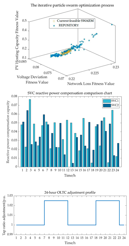
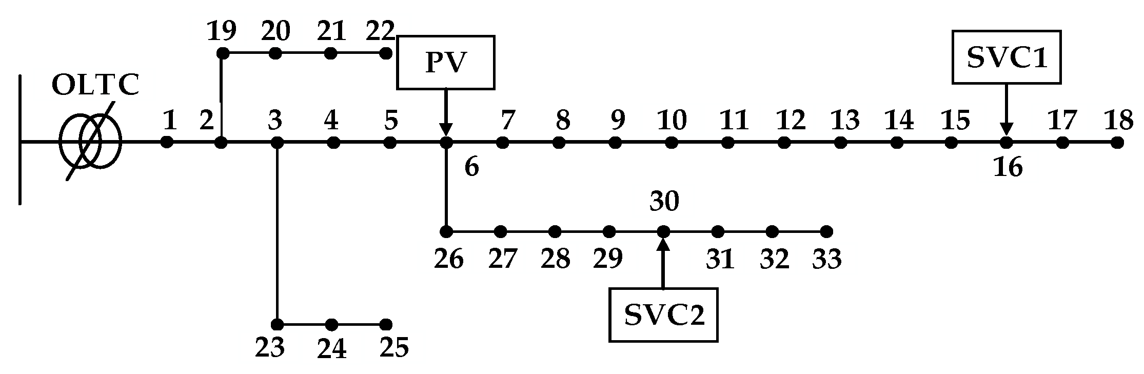
During periods of strong solar irradiation and low load demand, maximum PV output may cause voltage to rise at certain nodes, potentially exceeding permissible limits and threatening the safe operation of the distribution network. This issue is particularly pronounced in areas with weak network structures and insufficient reactive power regulation capability, where the indiscriminate integration of PV generation may result in voltage violations and system instability. Therefore, enhancing PV hosting capacity requires the effective participation of PV units in reactive power optimization. Common reactive power regulation methods include static var compensators (SVC), power capacitors, synchronous condensers, and on-load tap changers (OLTC). In this study, various reactive compensation devices are comprehensively coordinated within the distribution network to establish a reactive power optimization model tailored for high-penetration PV scenarios. The model aims to reduce voltage deviations and active power losses, thereby improving system stability and PV accommodation capability, and ultimately enhancing the overall operational efficiency of the distribution network.

2.1. Objective Function

(1) Active power loss of the distribution network $f_1$

$$f_1=\min {\displaystyle \sum _{i,j\in n}{r}_{ij}\frac{({P_{ij}}^2+{Q_{ij}}^2)}{U_i^2}}$$

(1)

where $n$ represents the number of nodes; $r_{ij}$ denotes the resistance between node $i$ and node $j$; $P_{ij}$ and $Q_{ij}$ represent the active power and reactive power, respectively, between node $i$ and node $j$; and $U_i$ is the voltage magnitude at node $i$.

(2) Voltage deviation of the distribution network $f_2$

$$f_2=\min {\displaystyle \sum _{t=1}^{24}{\displaystyle \sum _{i=1}^n{\left(\frac{U_{i,t}-U_i^{*}}{U_{i, \max }-U_{i,\min }}\right)}^2}}$$

(2)

where $U_{i,t}$ represents the voltage magnitude at node $i$ at time $t$; $U_i^{*}$ is the rated voltage of node $i$; and $U_{i, \max }$ and $U_{i,\min }$ represent the upper and lower voltage limits at node $i$, respectively.

(3) The photovoltaic (PV) absorption ratio of the distribution network $f_3$

$$f_3={\displaystyle \frac{{\displaystyle \sum _{i=1}^{24}{P}_{PV,t}^{use}}}{{\displaystyle \sum _{i=1}^{24}{P}_{PV,t}}}}\times 100\%$$

(3)

where $P_{PV,t}$ represents the photovoltaic power generation at time $t$ and $P_{PV,t}^{use}$ is the photovoltaic absorption power at time $t$.

2.2. Constraints

The constraints in reactive power optimization typically include equality and inequality constraints. The equality constraints in this study primarily involve power flow equations, while the inequality constraints encompass current and voltage limits as well as decision variable constraints. The decision variables include the hourly PV power injected into the grid over a 24 h period, the compensation capacity of reactive power compensators, and the tap positions of on-load tap-changing (OLTC) transformers. In distribution network reactive power optimization, control variables generally consist of both continuous and discrete variables. Continuous variables include generator reactive power output and the output of SVC/STATCOM devices, while discrete variables include transformer tap positions and capacitor bank switching states. The optimization process can simultaneously account for both continuous and discrete variables to ensure comprehensive and efficient reactive power control.

(1) Power flow constraints

$$\left\{\begin{array}{c}{P}_i+U_i{\displaystyle \sum _{j=1}^n{U}_j}(G_{ij}\cos {\theta }_{ij}+B_{ij}\sin {\theta }_{ij})={\displaystyle \sum _{i=n_{PV}}{P}_{PV,i}}\\ Q_i+U_i{\displaystyle \sum _{j=1}^n{U}_j}(G_{ij}\sin {\theta }_{ij}-B_{ij}\cos {\theta }_{ij})={\displaystyle \sum _{i\in n_{PV}}{Q}_{PV,i}+}{\displaystyle \sum _{i\in n_{SVC}}{Q}_{SVC,i}}\end{array}\right.$$

(4)

where $P_i$ and $Q_i$ represent the active and reactive power injections at node $i$, respectively; $G_{ij}$ denotes the conductance between node $i$ and node $j$; $B_{ij}$ is the susceptance between node $i$ and node $j$; $P_{PV,i}$ and $Q_{PV,i}$ represent the active and reactive power injected by the photovoltaic system at node $i$, respectively; ${\theta }_{ij}$ is the voltage phase angle difference between node $i$ and node $j$; and $n_{pv}$ and $n_{svc}$ represent the nodes where the photovoltaic system and reactive power compensator are connected, respectively.

(2) Current and voltage constraints

$$\left\{\begin{array}{c}{I}_{ij,\min }\le I_{ij,t}\le I_{ij,\max }\\ U_{i,\min }\le U_{i,t}\le U_{i,\max }\end{array}\right.$$

(5)

where $I_{ij,t}$ represents the current flowing between nodes $i$ and $j$ at time $t$; $I_{ij,\min }$ and $I_{ij,\max }$ are the minimum and maximum current limits flowing between nodes $i$ and $j$ at time $t$, respectively; $U_{i,t}$ is the voltage magnitude at node $i$ at time $t$; and $U_{i,\min }$ and $U_{i,\max }$ are the minimum and maximum voltage limits at node $i$, respectively.

(3) Decision variable constraints

$$\left\{\begin{array}{c}{Q}_{PV,i}^{\min }\le Q_{PV,i}\le Q_{PV,i}^{\max }\\ Q_{SVC,i}^{\min }\le Q_{SVC,i}\le Q_{SVC,i}^{\max }\\ T_i^{\min }\le T_i\le T_i^{\max }\\ Q_{C,i}^{\min }\le Q_{C,i}\le Q_{C,i}^{\max }\end{array}\right.$$

(6)

where $Q_{PV,i}^{\max }$ and $Q_{PV,i}^{\min }$ are the maximum and minimum reactive power injected by the photovoltaic system at node $i$, respectively; $Q_{SVC,i}^{\max }$ and $Q_{SVC,i}^{\min }$ are the maximum and minimum reactive power compensation capacities at node $i$, respectively; $T_i$ is the tap ratio of the $i$-th OLTC transformer; $T_i^{\max }$ and $T_i^{\min }$ are the maximum and minimum tap ratio limits of the $i$-th on-load tap-changer transformer; $Q_{C,i}$ is the reactive power compensation capacity at node $i$; and $Q_{C,i}^{\max }$ and $Q_{C,i}^{\min }$ are the maximum and minimum reactive power compensation capacities at node $i$, respectively.

3. Forecasting Photovoltaic Power Generation

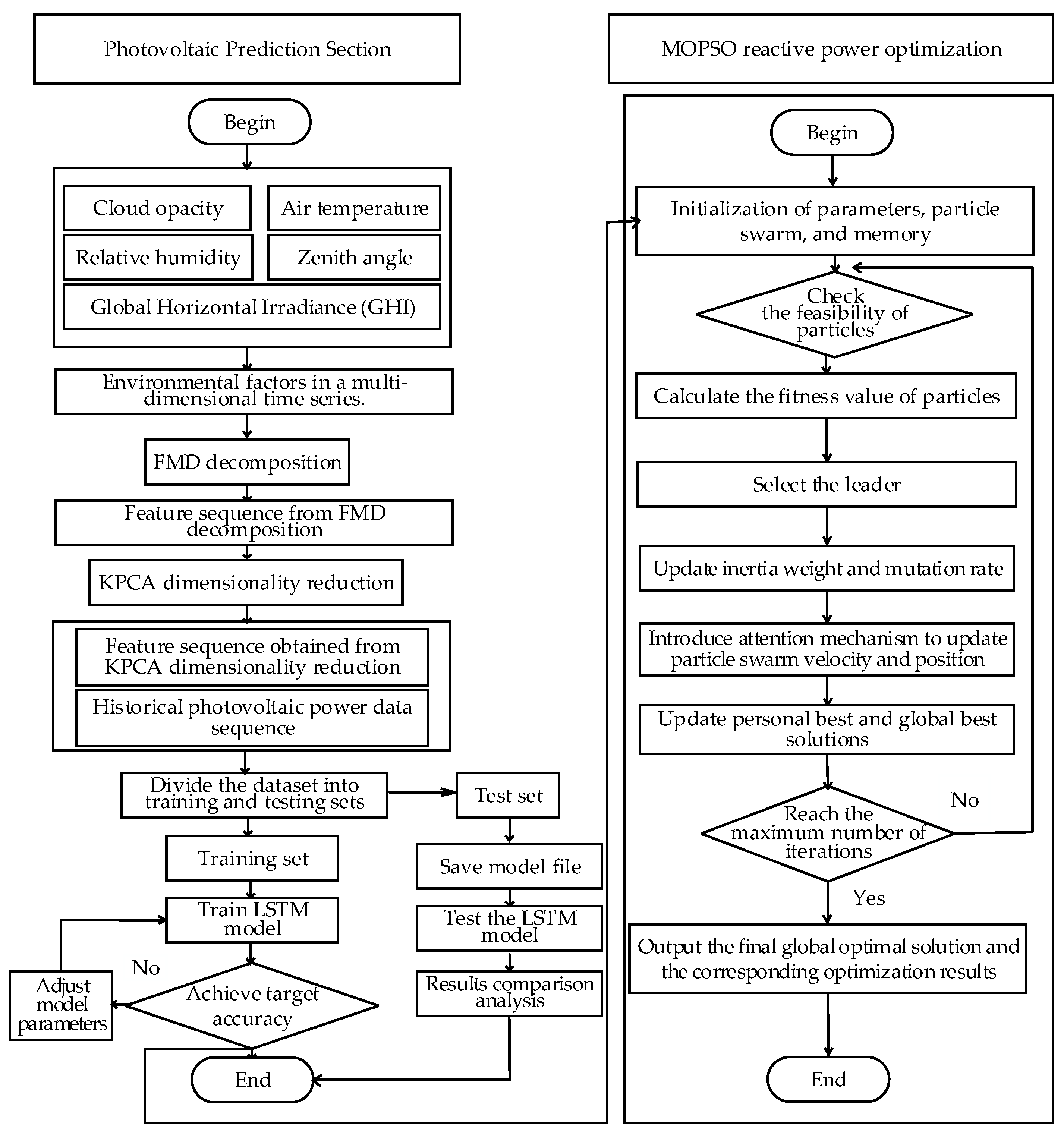
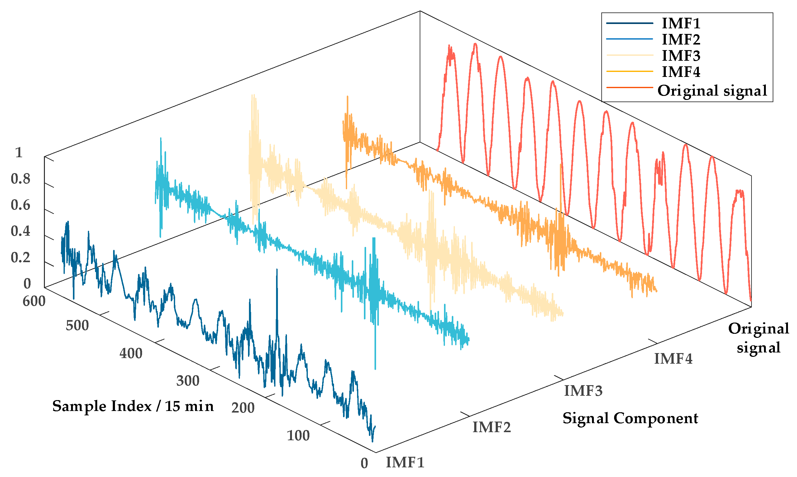
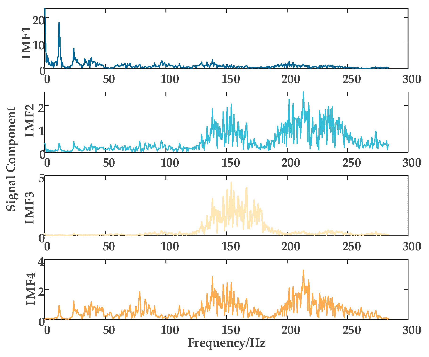
Short-term PV power forecasting provides critical support for enabling PV systems to participate in reactive power optimization. However, conventional signal decomposition methods, such as empirical mode decomposition (EMD) and variational mode decomposition (VMD), exhibit limitations when applied to non-stationary, multi-scale PV power signals. EMD is highly sensitive to noise and prone to mode mixing, resulting in decomposed components that lack clear physical interpretation. Although VMD can suppress mode mixing to some extent, it requires prior specification of the number of modes and penalty factors, which limits its adaptability and makes it less effective in handling complex spectral characteristics. To enhance the performance of hybrid forecasting models, this study first adopts an improved Feature Mode Decomposition (FMD) method to process environmental variables. Five environmental factors closely correlated with PV power output—global horizontal irradiance, air temperature, relative humidity, cloud optical depth, and solar zenith angle—are selected using Pearson correlation analysis. Each variable is decomposed into four modal components using the FMD approach. Subsequently, KPCA is applied to reduce the dimensionality of the high-dimensional feature space and extract the most informative characteristics. Finally, the dimensionally reduced features are fed into a LSTM network to achieve accurate PV power prediction.

3.1. Environmental Feature Decomposition Using an Improved FMD Model

The FMD method demonstrates strong noise and interference resistance by simultaneously considering the impulsive and periodic characteristics of the signal. This method utilizes an adaptive FIR filter to extract decomposition modes, overcoming the limitations of traditional methods related to filter shape, bandwidth, and center frequency, thereby achieving a more thorough signal decomposition. To address the non-stationarity and multi-scale features of PV power data, this study improves the FMD method by introducing an adaptive window function selection mechanism. Based on the spectral distribution characteristics of each frequency band, the mechanism dynamically selects either the Hanning window or the Blackman window, enabling more precise separation of short-term fluctuations and long-term trends in PV power.

Correlated kurtosis (CK) is used as an indicator to construct constraint conditions and update the FIR filter coefficients, decomposing the original signal into $k$ frequency bands, as defined by the following equation [30]:

$$\begin{gathered} \underset{\left\{f_k(l)\right\}}{\arg \max } \left\{C{K}_M(u_k)={\displaystyle \sum _{n=1}^N{({\displaystyle \prod _{m=0}^M{u}_k}(n-m{T}_p))}^2/{\left({\displaystyle \sum _{n=1}^N{u}_k}{(n)}^2\right)}^{M+1}}\right\} \\ \mathrm{s}.\mathrm{t}.u_k(n)={\displaystyle \sum _{l=1}^L{f}_k}(l)x(n-l+1) \end{gathered}$$

(7)

where $u_k(n)$ represents the $k$-th decomposition mode; $f_k$ is the $k$-th FIR filter function; $l$ denotes the index variable for the operation; $L$ is the filter length; $x(n)$ represents the original signal with length $N$; $T_p$ represents the photovoltaic fluctuation period; and $m$ is the shift order, $m\in [0,M]$.

The Hanning window and Blackman window are used to filter the low-frequency and high-frequency components of the signal, respectively. Under the constraint defined in the above Equation (7), the filter coefficients are updated iteratively with the maximum correlated kurtosis as the objective. The definition of the autocorrelation spectrum $R_x\left(\tau \right)$ is as follows [30]:

$$R_x(\tau )={\displaystyle {\int }_{n=1}^{N}x}(n)x(n+\tau )\mathrm{d}n$$

(8)

where $\tau$ is the lag coefficient.

First, the number of update iterations for the $k$-th filter is determined. Initial modal components are obtained through filter deconvolution. The correlation coefficients between the modal components are then calculated to identify the two pairs of modes with the highest correlation. Among these, the mode with the lower relative kurtosis is eliminated. After elimination, the filter coefficients of the remaining modes are updated, and the iteration continues until the number of modal components reaches the predefined value $n$, at which point the process is terminated. The relevant equations are given in Ref. [30]:

$$C{C}_{pq}={\displaystyle \frac{{\displaystyle \sum _{n=1}^N(u_p(}n)-{\overline{u}}_p)(u_q(n)-{\overline{u}}_q)}{\sqrt{{\displaystyle \sum _{n=1}^N(u_p(}n)-{\overline{u}}_p{)}^2}\sqrt{{\displaystyle \sum _{n=1}^N(u_q(}n)-{\overline{u}}_q{)}^2}}}$$

(9)

where $u_p$ and $u_q$ represent the two mode components, and ${\overline{u}}_p$ and ${\overline{u}}_q$ are the average values of the $u_p$ and $u_q$ mode components, respectively. The following illustrates the procedure of the improved FMD method.

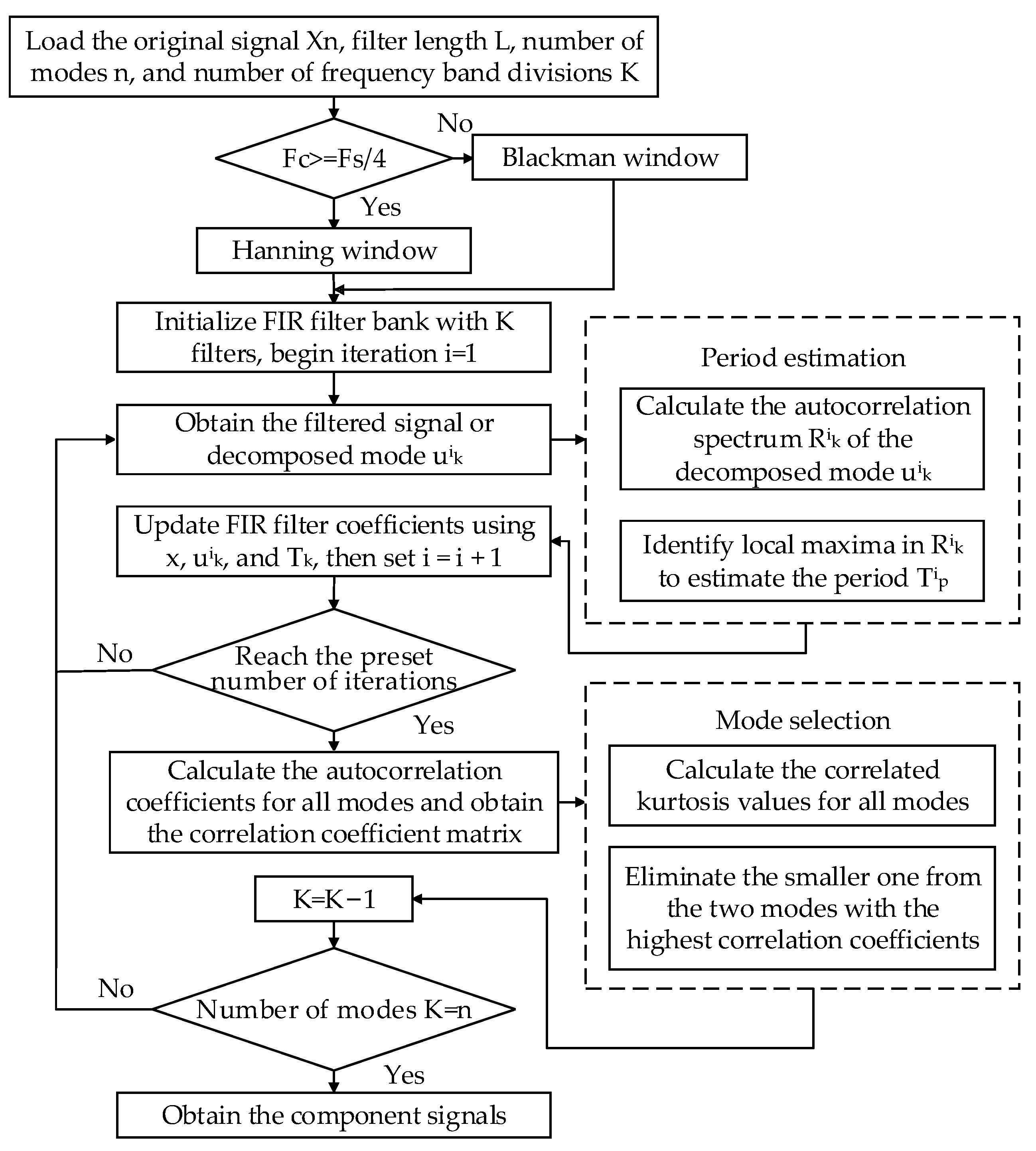
(1) Initialization: Load the original photovoltaic signal $x_n$, input preset parameters such as sampling frequency, filter size, the number of frequency bands, the number of decomposition modes, and the maximum number of iterations as input information for initialization. Define the frequency band range for each band. Based on the frequency band characteristics, dynamically select the window function: use the Hanning window for the high-frequency components and the Blackman window for the low-frequency components. Design $k$ FIR filters $f_k\left(l\right)$. Set the initial iteration counter $i=1$.

(2) Signal Decomposition: Filter the original signal $x_n$ using the filter group. Perform convolution operations on the signal using the filter group $f_k\left(l\right)$ to obtain the filtered mode components.

$$u_k^i\left(n\right)={\displaystyle \sum _{l=1}^L{f}_k\left(l\right)x\left(n-l+1\right)},k=1,2\dots ,K$$

(10)

Use the original signal $x_n$, the decomposition mode components $u_k^i\left(n\right)$, and the estimated photovoltaic fluctuation period $T_p$ to update the filter coefficients. The photovoltaic fluctuation period $T_p$ is estimated by the autocorrelation spectrum at the moment when it reaches the local maximum $R_k$ after the zero-crossing point. After one iteration, set $i=i+1$.

(3) Iteration Termination Check: Check whether the iteration count has reached the preset maximum iteration number. If it has not been reached, return to step 2 to continue the iteration. If it has been reached, proceed to step 4.

(4) Mode Component Selection: Use the Multiscale Decomposition Algorithm (MCKD) to decompose the signal into multiple modes (IMFs) and calculate the correlation coefficient between two modes:

$${\rho }_{ij} ={\displaystyle \frac{cov(x_{i },x_j )}{{\sigma }_{x_{i }} {\sigma }_{x_j}}}$$

(11)

where $cov(x_{i },x_j )$ is the covariance between signals $x_{i }$ and $x_j$, and ${\sigma }_{x_{i }}$ and ${\sigma }_{x_j}$ are the standard deviations of signals $x_{i }$ and $x_j$, respectively. This results in a matrix of size $K\times K$, representing the pairwise signal correlations. The correlation kurtosis of the two signals with the highest correlation coefficient is compared, and the signal with the higher correlation kurtosis is retained. By updating the signals and filters, redundant signals are removed, and the final $n$ modes are obtained. The improved FMD algorithm proposed in Ref. [30] follows the procedure illustrated in Figure 1.

3.2. Feature Dimensionality Reduction via KPCA

Excessively complex data can reduce the predictive performance of neural networks, making dimensionality reduction of the decomposed signals crucial to decrease computational complexity. Kernel Principal Component Analysis (KPCA) is an improvement on the PCA method. The core idea of KPCA is to map the data points in the input space to a feature space, where the data points in the feature space can be more easily processed and analyzed. Choosing an appropriate kernel function is critical for effective dimensionality reduction. Common kernel functions include linear kernel, polynomial kernel, and Gaussian kernel. Kernel functions also contain parameters that directly affect the degree of transformation, and these parameters can be determined through cross-validation. The explained variance method is used to evaluate the dimensionality reduction effect, and then the features obtained after KPCA fusion are ranked based on their contribution. The top few features whose total contribution reaches 90% of the overall contribution are selected as the reduced-dimensional data.

3.3. Long Short-Term Memory Network

LSTM is a deep learning algorithm based on an improved Recurrent Neural Network (RNN). The basic unit of LSTM is the memory block, which consists of three main stages: the forget stage, the input stage, and the output stage. Each stage has its specific operations, and the flow of information is controlled by different gating mechanisms.

3.4. Prediction Accuracy Evaluation

The model’s photovoltaic power prediction performance was evaluated using three metrics: Root Mean Square Error (RMSE), Mean Absolute Error (MAE), and the coefficient of determination (R²). The corresponding calculation formulas are provided in Appendix A.1.

4. A Reactive Power Optimization Model for Distribution Networks Based on an Improved MOPSO Algorithm

In the previous section, the PV forecasting model provided critical decision-making support for reactive power optimization by accurately predicting short-term photovoltaic generation. To further enhance the PV hosting capacity, this study develops a reactive power optimization model for distribution networks based on an improved multi-objective particle swarm optimization (MOPSO) algorithm. In this model, a multi-head attention mechanism is introduced into the particle velocity update process to enhance the algorithm’s global guidance and local exploration capabilities during the solution space search. The overall workflow is shown in Figure 2.

(1) After integrating static var compensators, photovoltaic generation, and on-load tap changers into the grid, the predicted photovoltaic output is used as the boundary for decision variables. Particle swarm initialization is performed, including acceleration coefficients, dynamic inertia weight, maximum iteration count, expansion rate, and dynamic mutation rate.

$$W(it)={\displaystyle \frac{({\max }_{\mathrm{iter}}-it)-(w_1-w_2)}{{\max }_{\mathrm{iter}}}}+w_2$$

(12)

$$pm(it)={\left(1-{\displaystyle \frac{it-1}{{\max }_{iter}-1}}\right)}^{{\displaystyle \frac{1}{\mu }}}$$

(13)

where $W(it)$ represents the dynamic inertia weight at iteration $it$; $w_1$ and $w_2$ denote the initial and final values of the inertia weight, respectively; ${\max }_{\mathrm{iter}}$ is the maximum number of iterations; $pm(it)$ denotes the dynamic mutation rate at iteration $it$; and $\mu$ represents the mutation rate.

The grid storage management is initialized, and individuals are assigned to the grid based on the objective function values.

$$\mathrm{Grid} \mathrm{Index}=⌊{\displaystyle \frac{f_i-f_{i,\min }}{f_{i,\max }-f_{i,\min }}}\times \mathrm{grid}\_\mathrm{size}⌋$$

(14)

where $f_i$ represents the $i$ objective function value; $f_{i,\min }$ and $f_{i,\max }$ denote the minimum and maximum values of the $i$ objective function, respectively; and $\mathrm{grid}\_\mathrm{size}$ represents the number of grids in each dimension.

(2) Based on the defined objective functions and constraints, the population and parameters are initialized to construct particle positions, update velocities, and assign attention weights.

$$\left\{\begin{array}{l}{X}_i=\left[x_{i1},x_{i2},\cdots ,x_{id}\right]\\ V_i=\left[v_{i1},v_{i2},\cdots ,v_{id}\right]\\ W_i=\left[w_{i1},w_{i2},\cdots ,w_{id}\right]\end{array}\right.$$

(15)

where $X_i$ represents the position vector of particle $i$, consisting of $d$ components; $V_i$ denotes the velocity vector of particle $i$; and $W_i$ represents the attention weight of particle $i$.

(3) Fitness Value Calculation

The iterative loop calculates the fitness function based on the objective functions of each particle to ensure that the voltage magnitude remains within the allowable range while optimizing system performance.

$$F_i=\left[f_{i1}{f}_{i2},\cdots ,f_{ik}\right]$$

(16)

where $f_{ik}$ represents the $k$-th fitness value of particle $i$.

A voltage violation penalty function is introduced into the network loss model to effectively constrain the voltage magnitude and enhance the stability and safety of the system.

$$F_0={\left({\displaystyle \frac{\Delta V_i}{V_{i,\max }-V_{i,\min }}}\right)}^2\cdot Z_1$$

(17)

where $F_0$ represents the voltage violation penalty value; $\Delta V_i$ is the voltage deviation at node $i$; $V_{i,\max }$ and $V_{i,\min }$ denote the lower and upper voltage limits at node $i$, respectively; and $Z_1$ is the penalty coefficient.

(4) The attention weight $W_i$ is optimized using evolutionary strategies, and iterative evolution is achieved using methods such as parent selection and new solution generation. During this process, the attention weights are dynamically adjusted, considering both the distance between particles and the historical optimal solution as well as the differences in fitness. This approach enhances the algorithm’s exploration ability in the search space and improves its convergence performance.

$$W_i^c,W_i^s=updateAttentionWeight(X_i^k,P_{bes{t}_i}^k,G_{best}^k,F_i)$$

(18)

where $W_i^c$ represents the cognitive component attention weight of particle $i$; $W_i^s$ denotes the social component attention weight of particle $i$; $X_i^k$ is the position of particle $i$ at iteration $k$; $P_{bes{t}_i}^k$ represents the individual historical best position of particle $i$ at iteration $k$; and $G_{best}^k$ is the global best position of the population at iteration $k$. See Appendix A.2 for the specific encapsulation formula.

(5) The particle velocity update employs an attention mechanism, where the cognitive and social coefficients are dynamically adjusted based on the historical best position and fitness values using multi-head attention weights, thereby updating the particle’s velocity and position.

$$\left\{\begin{array}{l}\begin{array}{l}{V}_i^{k+1}=W(it)\cdot V_i^k+c_1\cdot r_1\cdot (P_{bes{t}_i}^k-X_i^k)+c_2\cdot r_2\cdot (G_{best}^k-X_i^k)\\ X_i^{k+1}=X_i^k+V_i^{k+1}\end{array}\hfill \\ c_1=c_1^{\prime }\cdot W_i^c,c_2=c_2^{\prime }\cdot W_i^s\hfill \end{array}\right.$$

(19)

where $V_i^{k+1}$ represents the velocity of particle $i$ at iteration $k+1$; $r_1$ and $r_2$ are random numbers; $c_1$ is the dynamic cognitive coefficient; and $c_2$ is the dynamic social coefficient.

(6) During the position update stage, boundary constraints are introduced to correct the particle’s position, ensuring it remains within the predefined reasonable range.

(7) The individual best position is updated by comparing the current fitness value with the individual best position.

$$P_{bes{t}_i}=arg\min (F_i)$$

(20)

(8) If the current particle is not dominated by other particles, the global best solution is updated, and the external storage mechanism is updated accordingly.

$$G_{best}=arg\min (F)$$

(21)

(9) Finally, the current iteration count is checked to see if it has reached the maximum value. If the maximum iteration has not been reached, the algorithm continues to iterate; otherwise, the global optimal solution and optimization results are output.

5. Case Study Analysis

To verify the feasibility and effectiveness of the proposed model, a simulation study was conducted on the MATLAB 2018b platform using the modified IEEE 33-bus distribution system as the test system. The system operates at a voltage level of 12.66 kV, with a three-phase power base of 10 MVA. To reflect the characteristics of high-penetration PV integration, the total installed PV capacity was set to approximately 30% of the maximum active load in the distribution network—this ratio is commonly used as a threshold to define high-PV-penetration scenarios. However, excessive PV capacity, especially when connected near the end of feeder branches, can easily lead to voltage limit violations and associated control challenges. Considering the network topology and load distribution, a 1.2 MW PV plant was integrated at Bus 6. An OLTC was installed at Bus 1, with a voltage regulation range of [1.0, 1.1] p.u., a step size of 0.0125 p.u., and a total of 9 tap positions (0 to +8). Additionally, static var compensators with a capacity of 800 kvar were installed at Buses 16 and 30 to enhance reactive voltage support at the end of the feeder. The network topology is illustrated in Figure 3.

5.1. Prediction of Photovoltaic Output Based on the FMD-KPCA-LSTM Model

5.1.1. Experimental Data Preprocessing

The experimental data used in this study were collected from a photovoltaic (PV) power station located in Sichuan Province, China, covering the period from 24 September to 6 October 2020. The data were sampled at 15 min intervals, resulting in a total of 569 daytime records during periods with effective solar irradiance. The dataset includes the measured PV power output from Inverter No. 3, along with five corresponding environmental features: ambient temperature, relative humidity, cloud opacity, global horizontal irradiance (GHI), and solar zenith angle. The PV plant is situated in a northern, hilly region at an altitude exceeding 800 m and experiences a temperate continental climate with relatively stable weather conditions. The data were acquired from PV Array No. 20, which is centrally located within the plant and equipped with well-maintained monitoring devices, ensuring data reliability. To address potential anomalies arising from communication failures or other operational disturbances, daily data cleaning was conducted, and all records containing zero values for either power output or environmental parameters were removed. Since PV systems primarily generate power during daylight hours, the study period was restricted to the time interval between 07:00 and 19:00 each day.

5.1.2. Parameter Settings

The aforementioned FMD-KPCA-LSTM model was employed for photovoltaic power prediction. In the FMD signal decomposition, the filter size was set to 20, with 4 cut points and 4 modes, and the maximum number of iterations was 30. The KPCA utilized a polynomial kernel function with a kernel parameter of 1. Based on the scaled preprocessed data, experimental results verified its effective dimensionality reduction performance. For the LSTM network, the maximum number of training epochs was set to 100, with an initial learning rate of 0.01. After 70 epochs, the learning rate was adjusted. A regularization parameter of 0.01 was applied. The input layer had a time step of 1 and an input dimension of 5, the network consisted of a single hidden layer with 50 units, and the output layer dimension was 1. The training batch size was 25. The dataset was split into training and testing sets with a ratio of 7:3.

5.1.3. Analysis of Photovoltaic Output Prediction Results

(1) FMD Decomposition Results: The photovoltaic data exhibit certain periodicity and random fluctuations. To highlight its signal characteristics, the FMD decomposition is applied to extract feature signals, resulting in 539 × 20 sets of feature data. The decomposition signals of global horizontal radiation are selected for visualization analysis, as shown in Figure 4.

IMF1 primarily reflects the low-frequency trend, while IMF2 and IMF3 capture the mid-frequency components of the signal, representing mid-term fluctuations. IMF4 mainly contains high-frequency noise and interference. The spectral characteristics are comprehensively analyzed based on the time-frequency distribution presented in Figure 5.

From the spectrogram, it can be observed that the low-frequency components reflect the initial data trend, and that the mid-frequency fluctuations and the high-frequency noise are well separated. The spectra of the decomposed modes show clear separation characteristics, with low, mid, and high-frequency components either not overlapping or only minimally overlapping. Overall, the FMD decomposition performs well.

(2) KPCA Dimensionality Reduction Results: KPCA can construct a new feature space using a kernel function for data processing, retaining key data information while reducing the complexity and dimensionality of data processing. This improves the efficiency of machine learning algorithms. The specific decomposed signals are shown in

Table 1. Principal component contribution.

Component	Eigenvalue	Variance Contribution Rate (%)	Cumulative Contribution Rate (%)
1	1387.49	51.21	51.21
2	424.40	15.66	66.87
3	336.61	12.42	79.29
4	191.74	7.08	86.37
5	108.01	3.99	90.36
6	61.77	2.28	92.64
7	57.08	2.11	94.75
⁞	⁞	⁞	⁞
19	0.28	0.01	99.99
20	0.13	0.00	100.00

The first five components are selected as the initial data for prediction, corresponding to the cumulative contribution rate reaching 90%.

. Based on the decomposition results, KPCA is suitable for the photovoltaic forecasting process.

(3) Prediction Result Analysis: To evaluate the prediction performance of the proposed FMD-KPCA-LSTM model under transitional weather conditions, this study selected daytime data from three representative meteorological days in the test set: 5 October 2020 (overcast), 2 October 2020 (variable weather), and 3 October 2020 (sunny). Based on this dataset, three typical models were used as benchmarks for comparison: FMD-LSTM, Transformer, and the EMD-PCA-LSTM model proposed in Ref. [19]. The comparison between FMD-KPCA-LSTM and FMD-LSTM primarily aimed to examine the necessity of applying KPCA for dimensionality reduction to eliminate redundancy in meteorological data and improve prediction accuracy. In contrast, the comparison with the method from Ref. [19] highlights the advantages of the improved hybrid model and demonstrates the superior adaptability and expressive capability of FMD in decomposing photovoltaic power data. A visualization of the prediction results is shown in Figure 6.

As observed from the visualization results above, the proposed algorithm achieves the best fitting performance under all three weather conditions. The specific evaluation metrics are summarized in

Table 2. Comparison of evaluation indicators.

Comparison Model	Cloudy			Variable Weather			Sunny
	RMSE	MAE	R2/%	RMSE	MAE	R2/%	RMSE	MAE	R2/%
Transformer	7.3291	6.4384	0.9576	5.6605	4.6510	0.9642	6.6651	5.7735	0.9676
FMD-LSTM	3.3523	2.2126	0.9911	4.6225	3.4649	0.9761	2.1845	1.5989	0.9965
Ref. [19] method	2.9064	1.9532	0.9933	4.2737	3.0632	0.9796	1.8598	1.4441	0.9975
FMD-KPCA-LSTM	2.2764	1.5839	0.9959	3.2889	2.5875	0.9879	1.6647	1.3448	0.9980

.

The experimental results demonstrate that the FMD-KPCA-LSTM model significantly outperforms the benchmark models in terms of all error metrics under different weather conditions. Specifically, compared with the method in Ref. [19], the RMSE of the proposed model decreased from 2.9064, 4.2737, and 1.8598 to 2.2764, 3.2889, and 1.6647 under overcast, variable, and sunny weather conditions, respectively, corresponding to relative reductions of 21.70%, 23.03%, and 10.48%, thus indicating a notable improvement in forecasting accuracy. Across the three weather scenarios, the FMD-KPCA-LSTM model achieved an average RMSE of 2.4100 ± 0.1606, an average MAE of 1.8387 ± 0.1459, and an average R² of 0.998 ± 0.0005. The standard deviations reflect the performance variability of the model under different meteorological conditions, indicating that the proposed model possesses strong stability and generalization capability across various weather patterns. Although the FMD-LSTM model improves feature extraction through FMD decomposition, the potential issue of mode mixing in PV data limits its effectiveness and may even increase forecasting errors due to the added model complexity. In contrast, the FMD-KPCA-LSTM model further integrates KPCA-based dimensionality reduction on the basis of FMD-LSTM, effectively extracting nonlinear features from PV data. This leads to substantial improvements in RMSE, MAE, and R². Notably, under highly variable weather conditions (e.g., 2 October 2020), the FMD-KPCA-LSTM model captures the complex nonlinear characteristics of PV generation data more accurately, demonstrating superior robustness and adaptability, thereby providing a reliable data foundation for subsequent reactive power optimization.

5.2. Reactive Power Optimization in Distribution Networks Considering Photovoltaic Output

The forecasting result corresponding to Figure 6c (a sunny day on 5 October 2020) from the previous section is selected as the upper limit of PV power injected into the grid. The parameter settings refer to Ref. [28] and typical applications of the MOPSO algorithm in distribution network optimization: the learning factors are set to 0.1 and 0.2, respectively; the population size is 100; the initial and final inertia weights are set to 0.5 and 0.001, respectively; the number of non-dominated solutions is set to 100; and the maximum number of iterations is 150.

To verify the performance of the proposed algorithm, a comparative analysis was conducted against the Grey Wolf Optimizer (GWO), Genetic Algorithm (GA), and the improved Whale Optimization Algorithm from Ref. [29] in the context of reactive power optimization. Figure 7 illustrates the voltage distribution of the IEEE 33-bus system at the peak load period (Hour 20).

As shown in Figure 7, under the baseline scenario—where typical loads are connected but no optimization measures are applied—the voltage at certain nodes drops below the lower limit required for secure and stable operation. After applying the improved MOPSO algorithm, all node voltages are effectively maintained within the safe range of 0.95–1.05 p.u. In comparison with the GA, GWO, and the method proposed in Ref. [29], the improved MOPSO achieves the most notable voltage improvement near nodes 19 and 33, with an increase of approximately 3.8% relative to the unoptimized case. Figure 7 presents the voltage profile of node 33 over a 24 h period, further illustrating the superior voltage regulation capability of the proposed method. Figure 8 illustrates the variation in network losses under different algorithms over time, facilitating a temporal analysis of the optimization performance.

From the 9:00 to 19:00 period, as PV output participates in reactive power optimization, network losses are reduced. However, after 19:00, with the increase in load demand, PV output drops to nearly zero, and system network losses gradually rise. At this point, by increasing the transformer tap ratio using OLTC and incorporating SVC for reactive power compensation, network losses are effectively reduced. The total network loss is reduced by 37.5% compared to before optimization. The improved algorithm not only effectively reduces distribution network losses and enhances grid economy but also promotes sustainable energy development. Furthermore, the improvement in grid economy is also reflected in the enhanced ability to accommodate renewable energy. Figure 9 presents a comparison of different algorithms in terms of PV accommodation.

At the same time, the reactive power optimization using the improved MOPSO algorithm also enhanced the photovoltaic absorption rate. The specific optimization data are shown in

Table 3. Comparison of different algorithms’ performance.

Comparison Models	PV Absorption Rate/%	Voltage Deviation/p.u.	Active Power Loss/MW
GA	72.6318	73.4563	2.6033
GWO	76.4483	72.1570	2.4771
Ref. [29] method	78.8452	71.9604	2.4657
Improved MOPSO	89.2168	63.5803	2.1119

below.

As shown in the comparison results of PV utilization rates, the proposed improved MOPSO outperforms GA, GWO, and the method in Ref. [29]. By optimizing the reactive power compensation strategy, the proposed algorithm moderately curtails PV output around time step 15, where the injection is relatively high, while increasing PV utilization during other periods. This contributes to enhanced voltage stability and reactive power support capacity. Compared with Ref. [29], the proposed method improves the PV utilization rate by 13.15%, reduces the voltage deviation by 2.86%, and lowers the active power loss by 11.01%.

To further verify the effectiveness of the proposed reactive power optimization method, three comparative scenarios are designed: Scenario 1 involves no reactive power optimization under typical load access; Scenario 2 considers only the optimized PV power curve without additional reactive power control; and Scenario 3 adopts the reactive power optimization method proposed in this study. The objective function values for the three scenarios are calculated and compared. The 24 h voltage profiles of the 33-bus system are shown in Figure 10.

As shown in Figure 10, Scenario 3 demonstrates an overall improvement in voltage levels after optimization. Under typical load conditions and with the optimized PV integration, the voltage range falls within [0.965–1.05], with some values slightly below the acceptable voltage range of [0.95–1.05] for distribution networks. After applying the optimization in Scenario 3, the voltage range is adjusted to [0.943–1.05], ensuring that the voltages remain within a reasonable range. This optimization effect is mainly attributed to the introduction of the multi-head attention mechanism in the particle velocity update process. By dynamically adjusting the cognitive and social coefficients, this mechanism enhances both the global exploration capability and local exploitation efficiency of the algorithm, thereby improving convergence performance. As a result, the algorithm can identify optimal reactive power compensation strategies that meet the target objectives at each time step, effectively improving voltage stability. The optimization performance of the three scenarios is further compared in

Table 4. Comparison of different Scenarios’ performance.

Comparison of Schemes	PV Absorption Rate/%	Voltage Deviation/p.u.	Active Power Loss/MW
Scenario 1	-	94.9791	3.5106
Scenario 2	89.2168	89.2252	3.0351
Scenario 3	89.2168	63.5803	2.1119

.

Under the scenario of typical load conditions with optimized PV integration, active power losses and voltage deviation are reduced by 30.42% and 28.74%, respectively. By introducing the PV feed-in power as a decision variable in the dynamic reactive power compensation process, the optimization strategy can more accurately respond to PV output fluctuations, thereby further enhancing reactive power regulation capability. Additional optimization results are provided in Appendix B. These findings indicate that the proposed method not only reduces voltage deviation and network losses but also effectively improves the adaptability of distribution networks to variable PV output, promoting the efficient utilization of high-penetration renewable energy. For distribution system operators (DSOs), this method contributes to increasing PV accommodation capacity and power quality, lowering voltage regulation costs and the economic losses caused by power losses, and strengthening the operational robustness and control flexibility of the grid under high-penetration distributed PV scenarios.

6. Conclusions

This paper addresses the issues caused by the high penetration of PV systems in distribution networks, such as uncertainty in PV power forecasting, limited PV absorption, and reactive power imbalance. An adaptive FMD-based coordinated reactive power–voltage optimization method is proposed to tackle these challenges. The main conclusions are as follows:

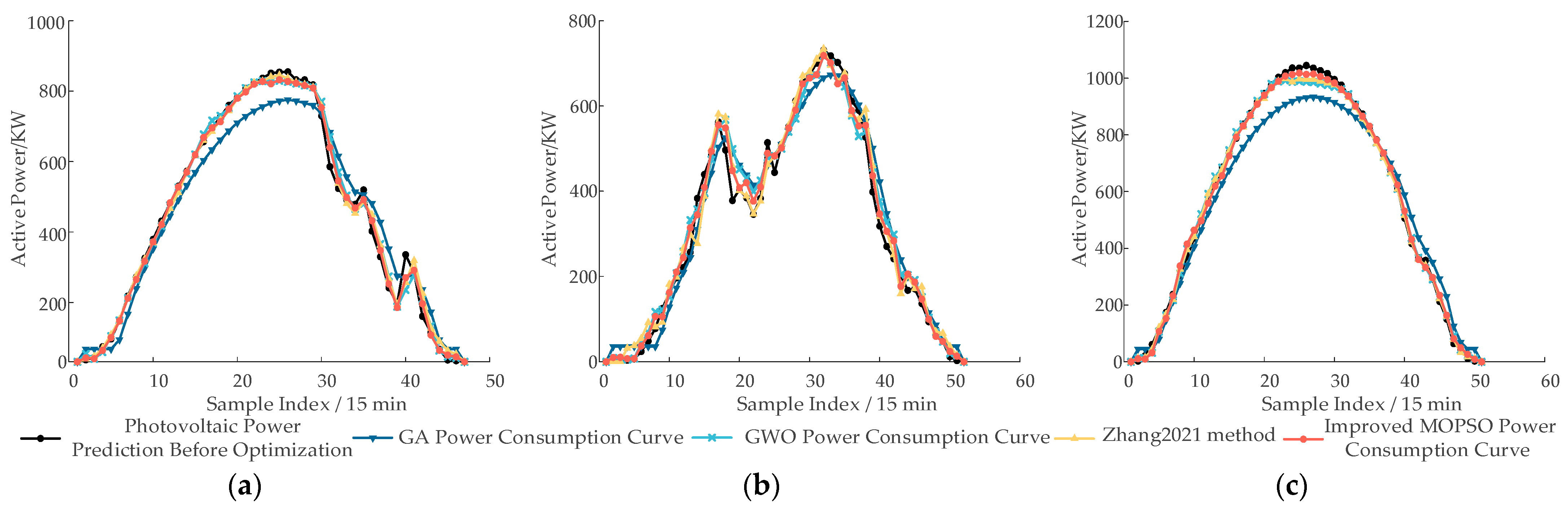
(1) The FMD based on an adaptive window function optimization enables more accurate extraction of the periodic fluctuations and long-term trends of photovoltaic (PV) output. Compared to the EMD-PCA-LSTM model reported in Ref. [19], the improved FMD-KPCA-LSTM forecasting method reduces the RMSE from 2.9064, 4.2737, and 1.8598 to 2.2764, 3.2889, and 1.6647 under cloudy, variable, and sunny conditions, respectively. This corresponds to accuracy improvements of 21.70%, 23.03%, and 10.48%, providing high-quality data support for subsequent reactive power optimization.

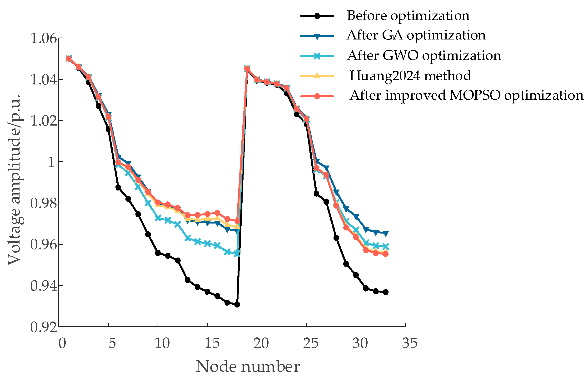
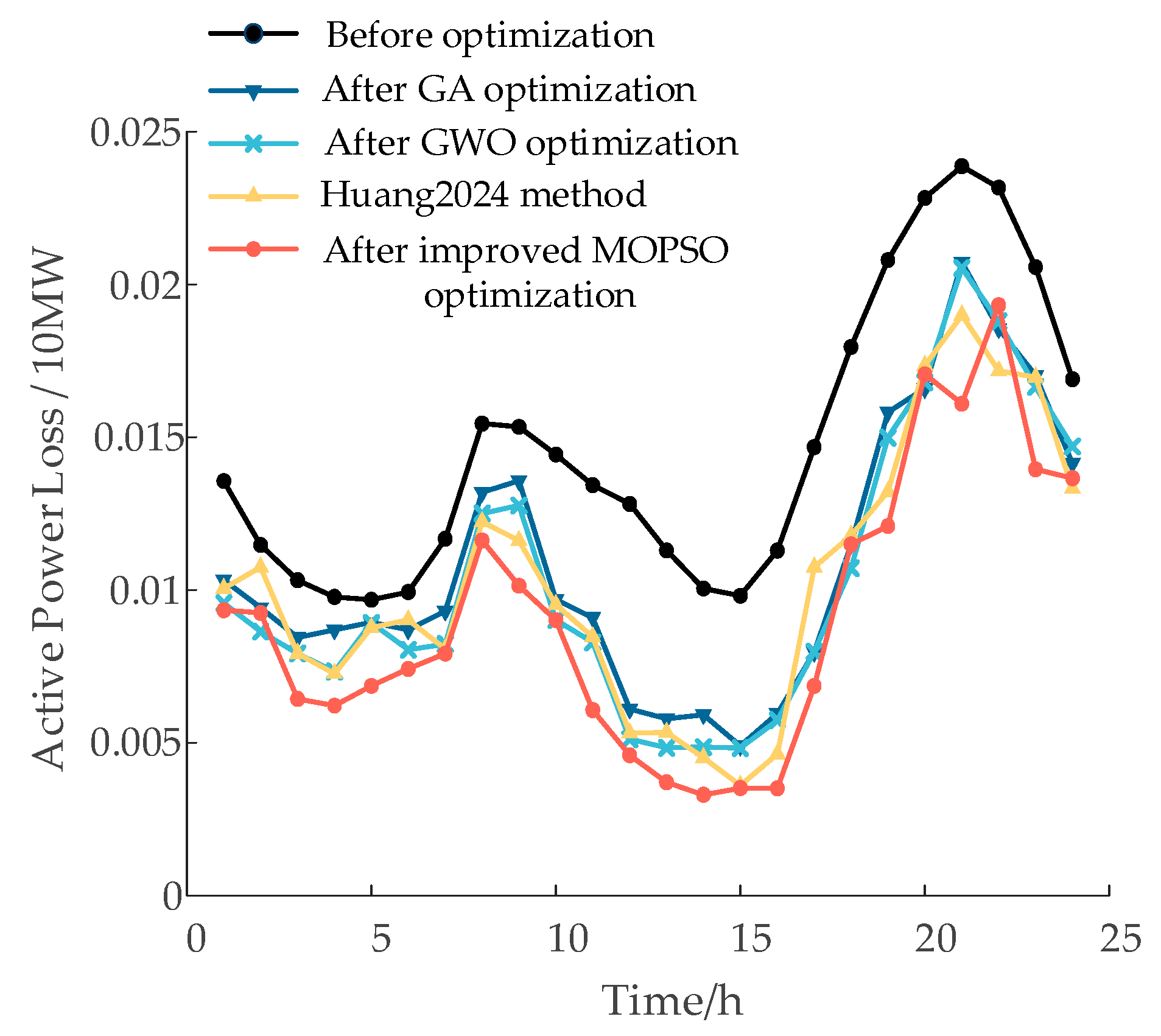
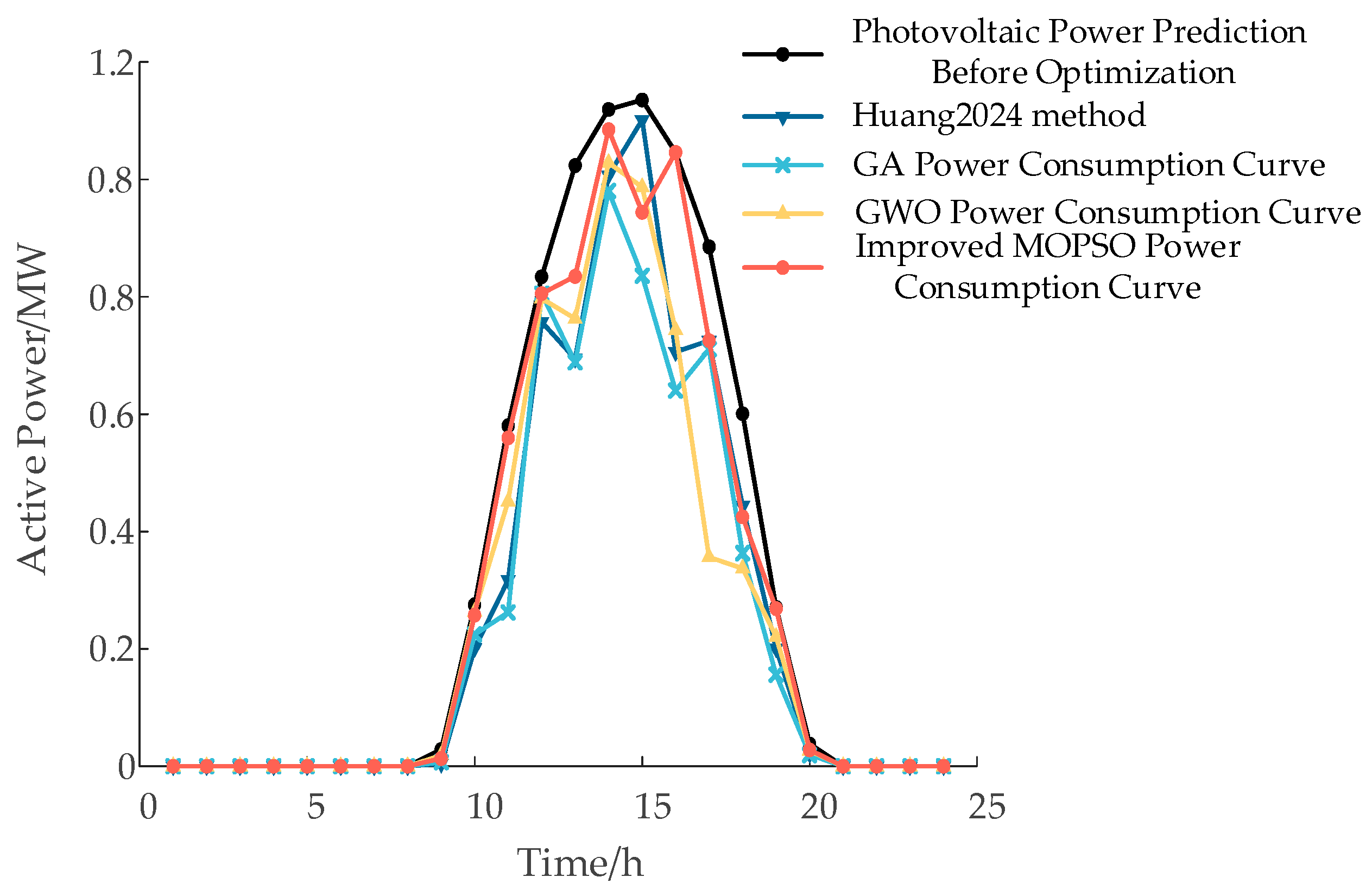
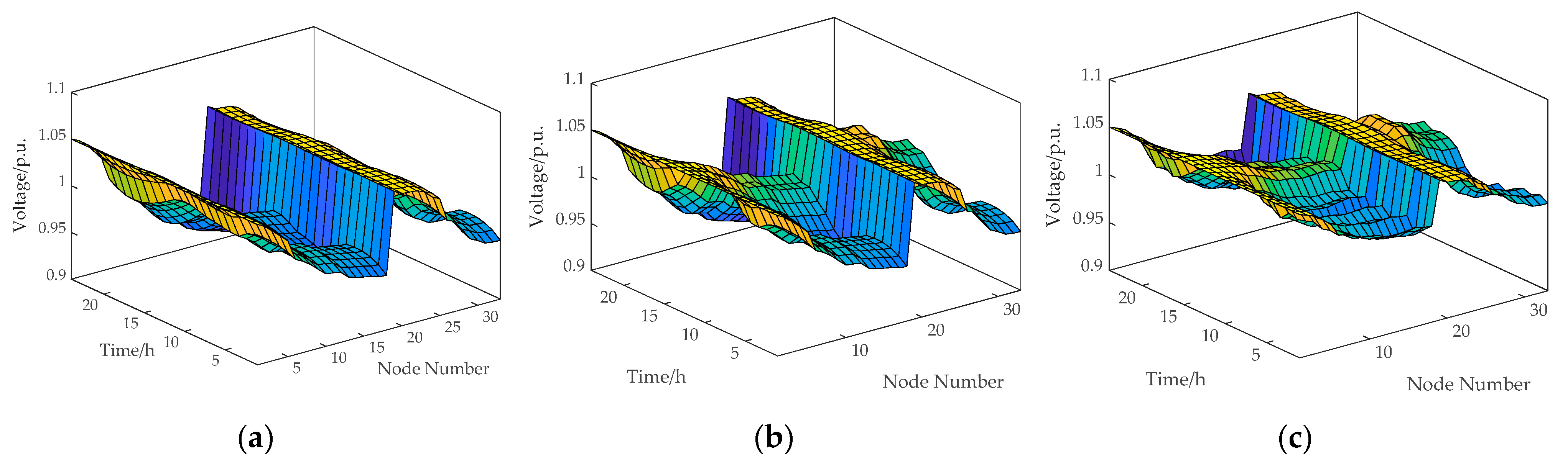
(2) A comprehensive objective function was constructed to coordinate the control of PV output, SVC, and OLTC, and solved using the improved MOPSO algorithm. Compared with the improved Whale Optimization Algorithm proposed in Ref. [29], the proposed method achieves a 13.15% increase in PV utilization rate, a 2.86% reduction in voltage deviation, and an 11.01% decrease in active power losses. Under the scenario with typical load and optimized PV integration, active power losses and voltage deviation are reduced by 30.42% and 28.74%, respectively. These results verify the effectiveness of the proposed method in minimizing network losses, enhancing PV accommodation, and improving voltage quality while satisfying voltage constraint conditions.

(3) Case study validation shows that the proposed method demonstrates superior adaptability and computational accuracy, effectively enhancing the safety and economy of the distribution network, and further highlights the important role of photovoltaic power forecasting in reactive power optimization.

This study focuses on reactive power optimization in a distribution network based solely on day-ahead typical load profiles and PV forecast data with a one-hour resolution, without fully considering the dynamic uncertainties present in actual dispatching. Future research could integrate time-of-use pricing mechanisms and extreme PV fluctuation scenarios to develop multi-time-scale dynamic secondary reactive power optimization under source-load uncertainties, thereby further enhancing scheduling flexibility and economic efficiency.