Air Conditioning Load Forecasting for Geographical Grids Using Deep Reinforcement Learning and Density-Based Spatial Clustering of Applications with Noise and Graph Attention Networks

Abstract

Air conditioning loads in power systems exhibit spatiotemporal heterogeneity across geographical regions, complicating accurate load forecasting. This study proposes a framework that integrates Deep Reinforcement Learning-guided DBSCAN (DRL-DBSCAN) clustering with a Graph Attention Network (GAT)-based Graph Neural Network to model spatial dependencies and temporal dynamics. Using meteorological features like temperature and humidity, the framework clusters geographical grids and applies GAT to capture spatial patterns. On a Pecan Street dataset of 25 households in Austin, the GAT with DRL-DBSCAN achieves a Test MSE of 0.0216 and MAE of 0.0884, outperforming K-Means (MSE: 0.0523, MAE: 0.1456), Hierarchical clustering (MSE: 0.0478, MAE: 0.1321), no-clustering (MSE: 0.0631, MAE: 0.1678), LSTM (MSE: 0.3259, MAE: 0.3442), Transformer (MSE: 0.6415, MAE: 0.4835), and MLP (MSE: 0.7269, MAE: 0.5240) baselines. This approach enhances forecasting accuracy for real-time grid management and energy efficiency in smart grids, though further refinement is needed for standardizing predicted load ranges.

1. Introduction

With the rapid development of renewable energy and accelerating urbanization, air conditioning loads have become a significant component of global energy consumption, particularly during peak summer periods. Studies indicate that air conditioning loads can account for over 50% of total electricity usage in certain regions [1], posing substantial challenges to power system stability and energy management. Accurate forecasting of air conditioning loads is essential not only for optimizing energy allocation, but also for enhancing grid stability and supporting demand response strategies. However, air conditioning loads are influenced by multiple factors, including temperature, humidity, and geographical location, exhibiting significant spatiotemporal heterogeneity. Notably, due to variations in climate conditions and regional development across different areas, air conditioning loads can differ markedly between regions. For instance, urban centers often experience higher loads due to the heat island effect and dense building layouts compared to suburban or rural areas. This spatial heterogeneity renders traditional forecasting methods, such as Autoregressive Integrated Moving Average (ARIMA) models [2] or Support Vector Regression (SVR) [3], inadequate in capturing regional load differences, resulting in suboptimal prediction accuracy.

In recent years, advancements in machine learning have provided new tools for load forecasting. Deep learning methods, such as Long Short-Term Memory (LSTM) networks, have been widely adopted for load forecasting due to their ability to handle sequential data [4]. However, these methods primarily focus on temporal dimensions and fail to adequately account for spatial dependencies. Research on spatial modeling has gained traction, with Convolutional Neural Networks (CNNs) being applied to model spatial correlations in electricity consumption across regions [5], and Graph Neural Networks (GNNs) capturing spatial relationships between buildings for energy consumption prediction [6]. Specifically, Graph Attention Networks (GATs), a variant of GNNs, have shown promise in load forecasting by effectively capturing spatial dependencies through attention mechanisms. For instance, a study employed GATs to model spatial relationships between wind farms for wind power prediction, integrating Transformer strategies to fuse multi-modal features and adaptively mine spatiotemporal dependencies at various scales [7]. Another study proposed a deep graph attention reinforcement learning network combining GATs with GRUs and Temporal Convolutional Networks (TCNs) for wind power forecasting, demonstrating improved accuracy in capturing spatial and temporal patterns [8]. These advancements highlight the potential of GATs in processing spatiotemporal data for load forecasting tasks.

Deep Reinforcement Learning (DRL) has also emerged as a powerful approach for load forecasting, particularly in optimizing energy management systems with spatiotemporal data. DRL techniques combine deep learning with reinforcement learning to handle complex control problems, making them suitable for dynamic load forecasting scenarios. A notable application of DRL in energy management involved the use of a Deep Q-Network (DQN) for short-term load forecasting (STLF), where a similar day selection method was developed to enhance prediction accuracy by learning optimal selection policies based on meteorological data [9]. Another study integrated DRL with gated recurrent units (GRUs) to form a DDPG-GRU model for STLF, adaptively optimizing hyperparameters to capture multi-dimensional load characteristics and improve forecasting performance in smart grids [10]. These studies underscore the DRL capability to address the temporal and spatial variability inherent in load forecasting, offering a promising direction for future research.

Load forecasting has been studied for decades, initially relying on statistical methods such as ARIMA [2] and exponential smoothing [11]. With the advent of machine learning, Support Vector Regression (SVR) [3] and Artificial Neural Networks (ANNs) [12] have become mainstream, offering improved capabilities to capture non-linear relationships. More recently, deep learning methods like LSTM [4] have gained prominence due to their effectiveness in handling sequential data. Spatiotemporal modeling has also progressed, with CNNs being used for electricity price forecasting [5] and GNNs for building energy consumption prediction [6]. Additionally, studies have highlighted the strong correlation between air conditioning loads and temperature, with models developed to incorporate temperature data [13] and integrate weather forecasts into ANN frameworks [14]. To further address the impact of meteorological and spatial factors on air conditioning load forecasting, recent research has focused on combining these elements. For example, a study analyzed the influence of meteorological factors such as temperature, humidity, wind speed, and precipitation on air conditioning loads, using Pearson’s correlation to select relevant inputs for a deep residual network, achieving a MAPE of 1.294% on the ISO-NE dataset [15]. Another study proposed a Temporal Convolutional Network (TCN) with attention mechanisms to model the non-linear relationship between meteorological factors (temperature, humidity, rainfall) and load, demonstrating improved forecasting accuracy by accounting for weather cumulative effects [16]. These studies emphasize the importance of integrating meteorological and spatial factors, yet they often treat spatial variations as secondary or aggregate data at higher levels (e.g., city-wide averages), overlooking fine-grained differences across geographical regions. In regions with extreme climates, research has focused more on the impact of weather variability on load patterns [17]. Clustering techniques have also been employed in load forecasting, such as clustering residential users based on load curves to improve short-term predictions [18] or using K-Means to identify industrial load patterns. However, studies combining spatial modeling with meteorological factors for air conditioning load forecasting remain scarce, particularly at the geographical grid level.

Existing studies fall short in integrating spatial modeling with air conditioning load forecasting, especially in addressing the interaction between geographical grids and meteorological factors. While traditional clustering methods can group similar loads, they often fail to incorporate spatial dependencies, and although GNNs show promise, their systematic integration with clustering for air conditioning load forecasting has not been thoroughly explored.

To address the spatial heterogeneity of air conditioning loads, this study integrates Deep Reinforcement Learning (DRL) and Density-Based Spatial Clustering of Applications with Noise (DBSCAN) to enhance load forecasting. DRL optimizes the DBSCAN parameter selection by modeling it as a Markov Decision Process (MDP), enabling adaptive clustering of geographical grids based on meteorological and geographical features. This approach ensures robust grouping of grids with similar load patterns, which is critical for accurate forecasting. Initially, the study area is discretized into geographical grids, which are subsequently clustered using the Deep Reinforcement Learning-guided DBSCAN (DRL-DBSCAN) framework proposed by Zhang et al. [19], incorporating meteorological features (e.g., temperature and humidity) to delineate regions exhibiting similar weather patterns and load characteristics. A GNN model, specifically implemented as a Graph Attention Network (GAT), is then employed to model the spatial dependencies and temporal dynamics among the grids, incorporating meteorological forecast data to enhance prediction accuracy. The GAT leverages an attention mechanism to dynamically weight the influence of neighboring grids, enabling more adaptive and precise modeling of spatial relationships. This methodology improves forecasting accuracy and provides detailed insights into load distribution, enabling more effective energy management strategies. The primary contributions of this study are three-fold:

1. Geographical Grid Clustering with DRL-DBSCAN: The DRL-DBSCAN framework is adopted to cluster geographical grids based on meteorological features, providing an automated and adaptive solution to address regional heterogeneity in air conditioning loads.

2. A GAT-based GNN is utilized to capture both spatial dependencies and temporal patterns within the grid structure, providing a robust framework for load forecasting by dynamically weighting the contributions of neighboring grids through an attention mechanism.

3. A novel air conditioning load forecasting framework is proposed, which simultaneously incorporates geographical information and meteorological data to improve prediction accuracy across diverse regions.

This study fills the gap between spatial modeling and air conditioning load forecasting at the geographical grid level, providing important theoretical and practical implications for smart grid applications.

2. Methods

2.1. Deep Reinforcement Learning and Density-Based Spatial Clustering of Applications with Noise (DRL-DBSCAN)

In the context of regional air conditioning load forecasting, spatial heterogeneity across geographical regions poses a significant challenge to clustering and prediction accuracy. The traditional density-based clustering algorithm, DBSCAN, relies on two critical parameters: the neighborhood radius (Eps) and the minimum number of points within that radius (MinPts). This approach is justified in load forecasting as it automates the clustering process, ensuring that geographical grids are grouped based on shared meteorological and geographical characteristics, which directly influence air conditioning load patterns. The DBSCAN density-based clustering is particularly suitable for load forecasting, as it forms non-spherical clusters and identifies noise points (e.g., isolated households with atypical loads), enhancing the spatial coherence of clusters used in subsequent GNN-based forecasting. To address the limitation of manual parameter tuning, we adopt the DRL-DBSCAN framework which models parameter selection as a Markov Decision Process (MDP) using deep reinforcement learning. This approach eliminates the need for manual intervention and adapts to varying data distributions, thereby enhancing the quality of geographical grid clustering and providing a robust foundation for subsequent load forecasting. The framework is shown in Figure 1.

The application of DRL-DBSCAN to geographical grid clustering involves the careful design of key reinforcement learning components, including the state space, reward function, and recursive mechanism, to ensure that the clustering results effectively support load forecasting. The state space is defined to capture both global and local clustering information, integrating meteorological and geographical features. Specifically, at the $i$-th step of the $e$-th episode, the global state $s_{\mathrm{global}}^{(e)(i)}$ is represented as a 7-tuple comprising the current parameter combination $P^{(e)(i)}=\{{\mathrm{Eps}}^{(e)(i)},{\mathrm{MinPts}}^{(e)(i)}\}$, the distances of the current parameters to their respective boundaries ${\mathcal{D}}_b^{(e)(i)}$, and the ratio of the number of clusters to the total number of grids $R_{cn}^{(e)(i)}={\displaystyle \frac{\left|{\mathcal{C}}^{(e)(i)}\right|}{\left|\mathcal{V}\right|}}$, where ${\mathcal{C}}^{(e)(i)}$ denotes the set of clusters and $\mathcal{V}$ represents the set of all grids. The local state $s_{\mathrm{local},n}^{(e)(i)}$ for each cluster $c_n\in \mathcal{C}$ is defined as a ($d$ + 2)-tuple, including the feature vector of the cluster center $X_{\mathrm{cent},n}^{(e)(i)}$ (comprising meteorological features such as average temperature and humidity, and geographical coordinates such as the grid center’s latitude and longitude), the Euclidean distance from the cluster center to the overall data center $D_{\mathrm{cent},n}^{(e)(i)}$, and the number of grids in the cluster $\left|c_n^{(e)(i)}\right|$. To integrate these states, an attention mechanism is employed to encode the global and local states into a fixed-length representation:

$$s^{(e)(i)}=\sigma \left(F_G\left(s_{\mathrm{global}}^{(e)(i)}\right)\Vert {\displaystyle \sum _{c_n\in \mathcal{C}}{\alpha }_{\mathrm{att},n}}\cdot F_L\left(s_{\mathrm{local},n}^{(e)(i)}\right)\right)$$

(1)

where $F_G$ and $F_L$ are fully connected networks for processing global and local states, respectively, $\sigma$ is the ReLU activation function, and ${\alpha }_{\mathrm{att},n}$ represents the attention weight for cluster $c_n$. This design ensures that the state space effectively captures the influence of meteorological and geographical features on clustering.

To improve the accuracy of load forecasting, the reward function guides the agent in selecting clustering parameters by using the Mean Squared Error (MSE) as the evaluation metric. MSE measures the discrepancy between the predicted load values (based on the current clustering results) and the actual load values, directly reflecting the impact of clustering quality on forecasting performance. The immediate reward at the $i$-th step is defined as follows:

$$\mathcal{R}\left(s^{(e)(i)},a^{(e)(i)}\right)=-\mathrm{MSE}\left(\widehat{Y},Y\right)$$

(2)

where $\widehat{Y}$ denotes the predicted load values derived from the clustering parameters $P^{(e)(i+1)}$ and DBSCAN results, and $Y$ represents the ground truth load data. The negative sign ensures that minimizing MSE corresponds to maximizing the reward. To encourage the agent to identify stable, high-quality clustering parameters over the long term, the final reward $r^{(e)(i)}$ combines the maximum future immediate reward and the reward at the episode’s endpoint:

$$r^{(e)(i)}=\beta \cdot \max {\left\{\mathcal{R}\left(s^{(e)(m)},a^{(e)(m)}\right)\right\}}_{m=i}^l+\delta \cdot \mathcal{R}\left(s^{(e)(l)},a^{(e)(l)}\right)$$

(3)

where $l$ is the final step of the episode, $\beta$ and $\delta$ are weighting factors balancing short-term and long-term rewards. This MSE-based reward design aligns the optimization of clustering parameters with the ultimate goal of load forecasting.

To address the computational complexity associated with large parameter spaces for Eps and MinPts, a recursive mechanism is implemented to progressively refine the parameter search. The parameter space is initially defined to cover the full range of possible values for Eps and MinPts (e.g., Eps from 0 to the maximum distance, and MinPts from 1 to the total number of grids). In subsequent layers, the search range is narrowed around the optimal parameters identified in the previous layer. Each layer employs a distinct DRL agent to search for the optimal parameter combination within the specified range, with the search step size ${\theta }_p^{(l)}$ (for Eps or MinPts) decreasing as the layer number increases, enabling coarse-to-fine adjustments. This recursive approach reduces the complexity of the parameter space from $O(N)$ to $O(\log N)$, where $N$ is the size of the parameter space, thereby improving computational efficiency while maintaining the precision of parameter selection. The resulting cluster labels are used to generate cluster embeddings, which, along with meteorological features, serve as input features for the Graph Attention Network (GAT) in the subsequent load forecasting step. This preprocessing step ensures that the spatial structure of the data reflects the meteorological and geographical factors driving air conditioning loads, providing a robust foundation for GAT to model spatial dependencies.

2.2. Graph Attention Network

Following the clustering of geographical grids using DRL-DBSCAN, which organizes regions based on shared meteorological and geographical characteristics, the subsequent phase involves modeling the spatial dependencies and temporal patterns inherent in these grids to achieve precise air conditioning load forecasting. Given the intrinsic spatial interconnections among grids—where neighboring grids often display correlated load behaviors due to common environmental and socioeconomic influences—a Graph Neural Network (GNN) with Graph Attention Network (GAT) layers is employed to effectively capture these relationships. This section elaborates on the application of GNNs, integrated with geographical data, to predict air conditioning loads across regional grids, maintaining coherence with the preceding methodology.

Conventional forecasting approaches, such as Long Short-Term Memory (LSTM) networks, adeptly model temporal dependencies but frequently neglect spatial correlations by treating each grid as an isolated entity. In the domain of air conditioning load forecasting, however, spatial proximity is a pivotal factor. For example, adjacent grids may exhibit similar load patterns influenced by comparable weather conditions or urban heat island effects. GNNs excel in managing relational data by representing geographical grids as nodes within a graph and their spatial relationships as edges. To address scalability, the GAT employs sparse attention mechanisms, making it suitable for larger graphs. Over-smoothing is mitigated by limiting the model to two GAT layers and applying dropout (rate 0.5), preserving node-specific features. Compared to alternatives like Graph Isomorphism Network (GIN), the GAT attention mechanism better captures nuanced spatial dependencies by dynamically weighting neighbor contributions, as validated in our experiments. This structure enables the model to propagate information across the grid network, allowing for simultaneous learning from localized features and broader spatial contexts.

To implement the GNN within the geographical grid framework, a graph is constructed:

$$\mathcal{G}=(\mathcal{V},\mathcal{E})$$

(4)

where $\mathcal{V}$ denotes the set of grid nodes and $\mathcal{E}$ represents the edges linking these nodes. Each node $v_i\in \mathcal{V}$ corresponds to a geographical grid, characterized by features such as meteorological data and geographical coordinates, and clustering labels derived from DRL-DBSCAN. Historical load data for each grid are also integrated into the node features to encapsulate temporal trends.

The edges $\mathcal{E}$ are defined based on geographical proximity, where two nodes $v_i$ and $v_j$ are connected if their Euclidean distance $d_{ij}$, computed using their latitude and longitude, is less than a predefined threshold $ϵ$:

$$d_{ij}=\sqrt{{({\mathrm{lat}}_i-{\mathrm{lat}}_j)}^2+{({\mathrm{lon}}_i-{\mathrm{lon}}_j)}^2}$$

(5)

To enhance the graph structure, the clustering results from DRL-DBSCAN are incorporated to modulate edge connections. Specifically, nodes within the same cluster are prioritized for connection, as they are assumed to share similar load behaviors due to their geographical and meteorological similarities. In contrast to traditional GCN-based approaches that rely on manually defined edge weights, the GAT model dynamically computes attention weights for each edge, eliminating the need for a predefined weighting scheme. The GAT leverages an attention mechanism to model spatial dependencies among geographical grids. For each node (representing a grid), GAT computes attention coefficients for its neighbors using a self-attention mechanism, which evaluates the relevance of neighboring features (e.g., meteorological data and historical load). These coefficients enable a weighted aggregation of neighbor information, allowing the model to prioritize grids with stronger spatial correlations, such as those with similar weather patterns due to proximity. This attention-based approach enhances the model’s ability to capture complex spatial relationships, improving load forecasting accuracy. This adaptive mechanism allows the model to focus on the most relevant neighbors during information propagation, enhancing its ability to capture spatially coherent patterns identified by DRL-DBSCAN. The resulting adjacency matrix is used directly in the GAT layers without additional normalization, as the attention mechanism inherently handles the weighting process.

The node features are carefully designed to encapsulate both spatial and temporal information. For each node $v_i$ at time $t$, the feature vector is defined as follows:

$$x_{i,t}=[l_{i,t-\tau :t},m_{i,t},c_i,{\mathrm{lat}}_i,{\mathrm{lon}}_i]\tau$$

(6)

where $l_{i,t-\tau :t}$ represents the historical load data over the past $\tau$ time steps, $m_{i,t}$ includes meteorological features such as temperature and humidity at time $t$, $c_i$ is the cluster label assigned by DRL-DBSCAN, ${\mathrm{lat}}_i$ and ${\mathrm{lon}}_i$ are the geographical coordinates. The inclusion of the cluster label $c_i$ allows the GAT to differentiate between grids belonging to distinct geographical clusters, thereby enhancing its ability to capture spatially coherent load patterns. The geographical coordinates provide explicit spatial context, enabling the model to account for location-specific influences, such as urban density or proximity to water bodies, which may affect air conditioning demand.

As shown in Figure 2, this study adopts a Graph Attention Network (GAT)-based GNN model, which refines each node’s representation by dynamically aggregating information from its neighbors using an attention mechanism. The GAT layer is mathematically expressed as follows:

$$H^{(l+1)}=\sigma \left(\widehat{A}{H}^{(l)}{W}^{(l)}\right)$$

(7)

where $H^{(l)}$ is the node feature matrix at layer $l$, $\widehat{A}$ is the normalized adjacency matrix of the graph, $W^{(l)}$ is the trainable weight matrix, and $\sigma$ denotes the activation function (ReLU). By stacking multiple GCN layers, the model captures higher-order spatial dependencies. In this implementation, the GAT consists of two layers: the first layer uses 4 attention heads with a hidden size of 32 per head (resulting in a concatenated output dimension of 128), and the second layer uses a single head with a hidden size of 32. A fully connected layer follows to produce the final load predictions. The ReLU activation function is applied after each GAT layer to introduce non-linearity, and dropout is incorporated to prevent overfitting, with a dropout rate of 0.5. The prediction task is to forecast the air conditioning load for each grid at the next time step $t$, given the graph $G$ and the node features $X_t$. The GAT-GNN model can be formulated as follows:

$${\widehat{l}}_{t+1}=f_{\mathrm{GAT}}(G,X_t)$$

(8)

where ${\widehat{l}}_{t+1}$ is the predicted load vector for all nodes at time $t+1$, and $f_{\mathrm{GAT}}$ represents the GAT-GNN model. The model is trained using the MSE loss function, optimized with the Adam optimizer at a learning rate of 0.005 and a weight decay of $1\times {10}^{-3}$ to regularize the model parameters.

While the GAT layers primarily capture spatial dependencies through the attention mechanism, the temporal dynamics are implicitly modeled through the historical load data included in the node features. This approach allows the GAT to learn short-term temporal patterns, such as daily load fluctuations, while focusing on spatial relationships. To further enhance the model’s capacity to discern complex spatial patterns, positional encodings or spatial embeddings are incorporated into the node features. Specifically, the geographical coordinates are used to compute spatial embeddings, which provide explicit spatial context to the GAT. These embeddings can be generated using a simple linear transformation of the coordinates or through more advanced techniques such as sinusoidal positional encodings, ensuring that the model captures both relative and absolute positional information.

2.3. Integration Workflow for Air Conditioning Load Forecasting

The DRL-DBSCAN and GAT components are integrated into a unified workflow specifically designed for air conditioning load forecasting, effectively addressing the challenges of spatiotemporal heterogeneity and meteorological influences. The process unfolds as follows:

Spatial Clustering with DRL-DBSCAN: The geographical grids, defined by their latitude and longitude, are first clustered using DRL-DBSCAN. The clustering process incorporates meteorological features alongside spatial coordinates to identify regions with similar air conditioning load patterns. For instance, urban grids with high temperatures due to the heat island effect are grouped together, reflecting their increased cooling demands. DRL optimizes the DBSCAN parameters (Eps and MinPts) to ensure robust clustering, minimizing noise points (e.g., grids with anomalous loads due to extreme weather events) and maximizing the quality of clusters, as measured by the silhouette score. The resulting cluster labels are then embedded into a low-dimensional feature space (e.g., using an embedding layer with dimension 8), capturing the spatial structure of load patterns.

Graph Construction: Using the cluster labels from DRL-DBSCAN, a graph structure is constructed for GAT. Nodes represent geographical grids, and edges are defined based on two criteria: (a) grids within the same cluster are connected, as they share similar load and meteorological characteristics, and (b) spatially proximate grids are connected using a K-Nearest Neighbors (KNNs) approach (k = 3), with edge weights determined by their spatial distance and meteorological similarity (inverse of Euclidean distance in the meteorological feature space). This graph structure ensures that GAT can model both spatial dependencies and meteorological influences relevant to air conditioning loads.

Feature Preparation: Each node’s feature vector combines the meteorological features with the cluster embeddings from DRL-DBSCAN. These features enable GAT to capture the direct impact of weather conditions on air conditioning loads (e.g., higher temperatures leading to increased demand) while leveraging the spatial clustering information to enhance the modeling of regional effects (e.g., urban vs. rural load variations).

Load Prediction with GAT: GAT processes the graph and node features to predict air conditioning loads for each grid. Its attention mechanism assigns higher weights to neighboring grids with significant influence (grids with similar weather conditions or spatial proximity), allowing the model to focus on the most relevant spatial dependencies. For example, a grid in a densely populated urban area may exhibit higher loads due to heat retention, and GAT can capture this influence by prioritizing connections to nearby urban grids with similar meteorological profiles. The predicted loads are then compared to ground truth values, and the prediction error is computed.

Feedback Optimization with DRL: To further enhance performance, the prediction error from GAT is used as feedback to refine the DRL-DBSCAN clustering. Specifically, the MSE is incorporated into the DRL reward function, encouraging adjustments to eps and minpts that lead to better clustering outcomes (clusters that improve the GAT prediction accuracy). This closed-loop optimization ensures that the framework continuously adapts to the dynamic nature of air conditioning loads, improving overall forecasting performance over time.

This integrated workflow leverages the strengths of DRL-DBSCAN and GAT to address the specific challenges of air conditioning load forecasting: DRL-DBSCAN captures spatial patterns driven by meteorological factors, GAT models the spatial dependencies and meteorological influences, and the feedback loop ensures adaptive optimization, resulting in accurate and robust load predictions across geographical grids, as demonstrated in Section 3.

3. Case Study

To evaluate the effectiveness of the proposed DRL-DBSCAN and GAT-GNN framework for air conditioning load forecasting, a comprehensive case study is conducted using a real-world dataset of household energy consumption. This section details the experimental setup, including data preparation, model training, and evaluation metrics, followed by an in-depth analysis of the results. The primary objective is to assess the ability of the proposed framework to capture both spatial and temporal dependencies in the geographical grids, leveraging the clustering results from DRL-DBSCAN to enhance the GAT-GNN predictive performance.

3.1. Experimental Setup

The dataset used in this study comprises hourly air conditioning load data from 25 households in Austin, sourced from the Pecan Street project [20], collected over a period of one year. Each record includes the timestamp, household ID, geographical coordinates (latitude and longitude), meteorological features (local temperature and humidity), and the adjusted load. The data are aggregated at an hourly granularity to reduce noise and capture meaningful temporal patterns. To ensure consistency, the adjusted load values are standardized using a StandardScaler, and the meteorological features are similarly normalized to facilitate model training.

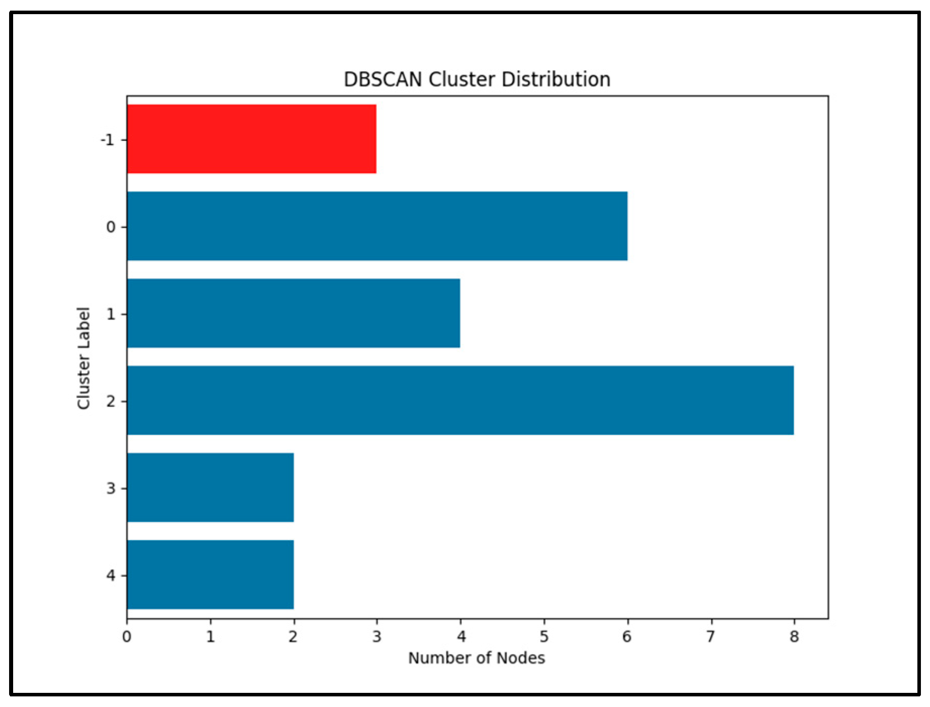
The geographical grids are constructed based on the latitude and longitude of each household, with each household representing a node in the graph. The DRL-DBSCAN algorithm is applied to cluster these nodes into spatially coherent groups, using an eps value of 0.07 and a minpt value of 2, determined through iterative experimentation to balance the number of clusters and noise points. 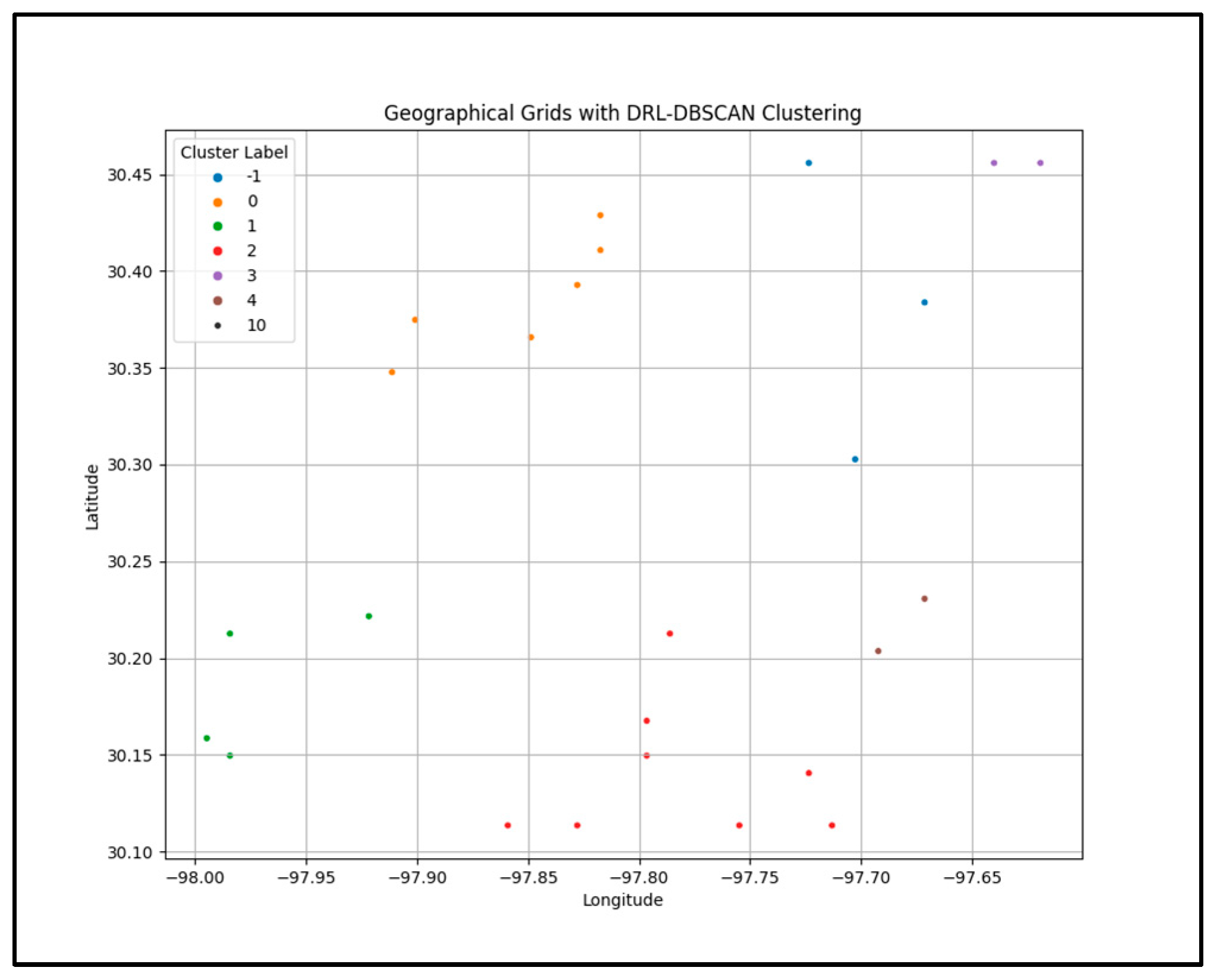The resulting clustering distribution, as shown in Figure 3, identifies five clusters: Cluster 0 (seven nodes), Cluster 1 (five nodes), Cluster 2 (eight nodes), Cluster 3 (one node), and Cluster 4 (one node), with three nodes labeled as noise (Cluster 1). The geographical distribution of these clusters, illustrated in Figure 4 demonstrates that the clusters effectively capture spatially proximate regions, which is critical for the subsequent GAT-based load forecasting.

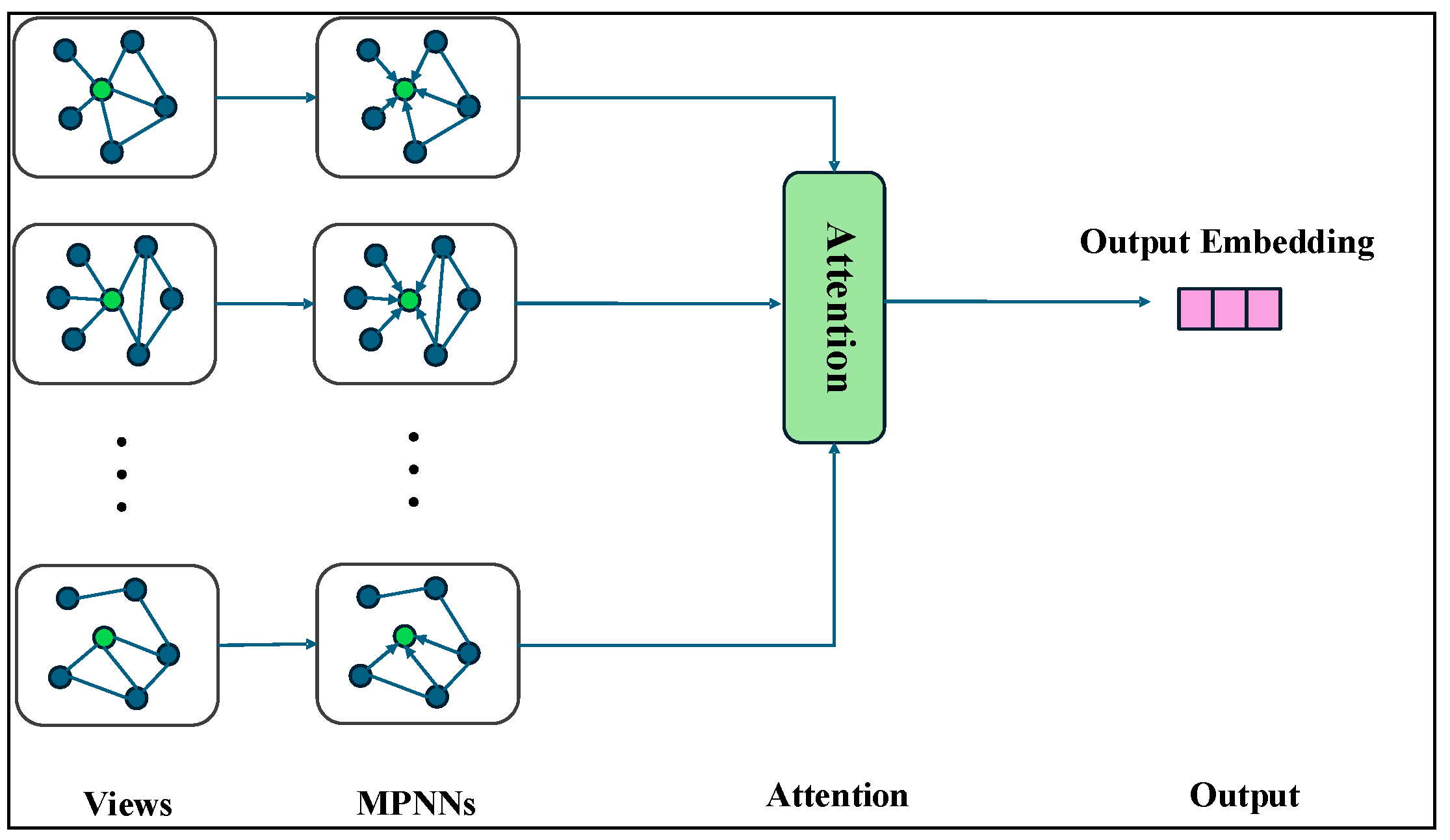
The GNN model is designed as a Graph Attention Network (GAT) with two GAT layers to capture higher-order spatial dependencies among the geographical grids. The first GAT layer uses four attention heads with a hidden size of 32 per head (resulting in a concatenated output dimension of 128), followed by a second GAT layer with a single head and a hidden size of 32. A final fully connected layer maps the output to the predicted load. The node features include the local temperature, humidity, and a four-dimensional embedding of the cluster label, which enhances the model’s ability to differentiate between spatially distinct groups. The graph structure is constructed by connecting nodes within the same cluster if their Euclidean distance is less than 0.05. In contrast to traditional GCNs, the GAT model dynamically computes attention weights for each edge, eliminating the need for manually specified edge weights, which allows for more adaptive information propagation within clusters, reflecting the spatial coherence identified by DRL-DBSCAN.

3.2. Evaluation Metrics

The performance of the models is evaluated using two standard metrics: Mean Squared Error (MSE) and Mean Absolute Error (MAE). These metrics are computed on both the training and testing sets to assess the models’ predictive accuracy and generalization ability. Additionally, heatmaps of the predicted loads are generated to visualize the spatial distribution of the predictions, providing insights into the models’ ability to capture spatial patterns.

3.3. Comparison of Different Clustering Methods

To evaluate the effectiveness of the proposed DRL-DBSCAN clustering method in enhancing the GAT-GNN ability to capture spatial dependencies for air conditioning load forecasting, a comparative study is conducted by integrating different clustering algorithms into the GAT-GNN framework. The objective of this experiment is to assess how the choice of clustering method impacts the GAT-GNN predictive performance and its ability to model spatial patterns. Four clustering approaches are considered: (1) the proposed DRL-DBSCAN, (2) K-Means clustering, (3) Hierarchical clustering with Ward linkage, and (4) a baseline scenario without clustering (using raw geographical coordinates directly). Each clustering method is applied to the same dataset of 25 geographical grids, and the resulting cluster labels are incorporated into the GAT-GNN node features as described in Section 2.2. The GAT-GNN architecture, graph structure, and training settings remain consistent across all experiments to ensure a fair comparison.

The DRL-DBSCAN algorithm is configured with eps = 0.07 and minpt = 2, yielding five clusters (Cluster 0: seven nodes, Cluster 1: five nodes, Cluster 2: eight nodes, Cluster 3: one node, Cluster 4: one node) and three noise points (Cluster 1), as previously shown in Figure 3. For K-Means clustering, the number of clusters is set to five to match the number of non-noise clusters produced by DRL-DBSCAN, and the algorithm is initialized with the k-means++ method to ensure robust convergence. Hierarchical clustering is performed using Ward linkage, also producing five clusters by cutting the dendrogram at an appropriate level. In the no-clustering baseline, the cluster label feature is omitted from the node features, and the GAT-GNN relies solely on the geographical coordinates (latitude and longitude) to capture spatial relationships. The GAT-GNN model is trained and evaluated for each clustering method, following the setup described in the previous subsection. The performance is assessed using the Mean Squared Error (MSE) and Mean Absolute Error (MAE) on both the training and test sets. Additionally, the spatial distribution of the predicted loads is visualized to analyze how different clustering methods influence the GAT-GNN ability to capture spatially coherent load patterns.

The predictive performance of the GAT-GNN with different clustering methods is summarized in

Table 1. Performance of GAT-GNN with different clustering methods.

Clustering Method	MSE	MAE
DRL-DBSCAN	0.0388	0.1559
K-Means	0.0731	0.2151
Hierarchical	0.0502	0.1883
No-Clustering	0.0813	0.2584

. The GAT-GNN with DRL-DBSCAN achieves the best performance on the test set, with a test MSE of 0.0388 and a test MAE of 0.1559. In contrast, the GAT-GNN with K-Means clustering yields a test MSE of 0.0731 and a test MAE of 0.2151, while Hierarchical clustering results in a test MSE of 0.0502 and a test MAE of 0.1883. The no-clustering baseline performs the worst, with a test MSE of 0.0813 and a test MAE of 0.2584. These results indicate that DRL-DBSCAN significantly enhances the GAT-GNN predictive accuracy compared to other clustering methods, likely due to its ability to identify spatially coherent clusters while handling noise points effectively.

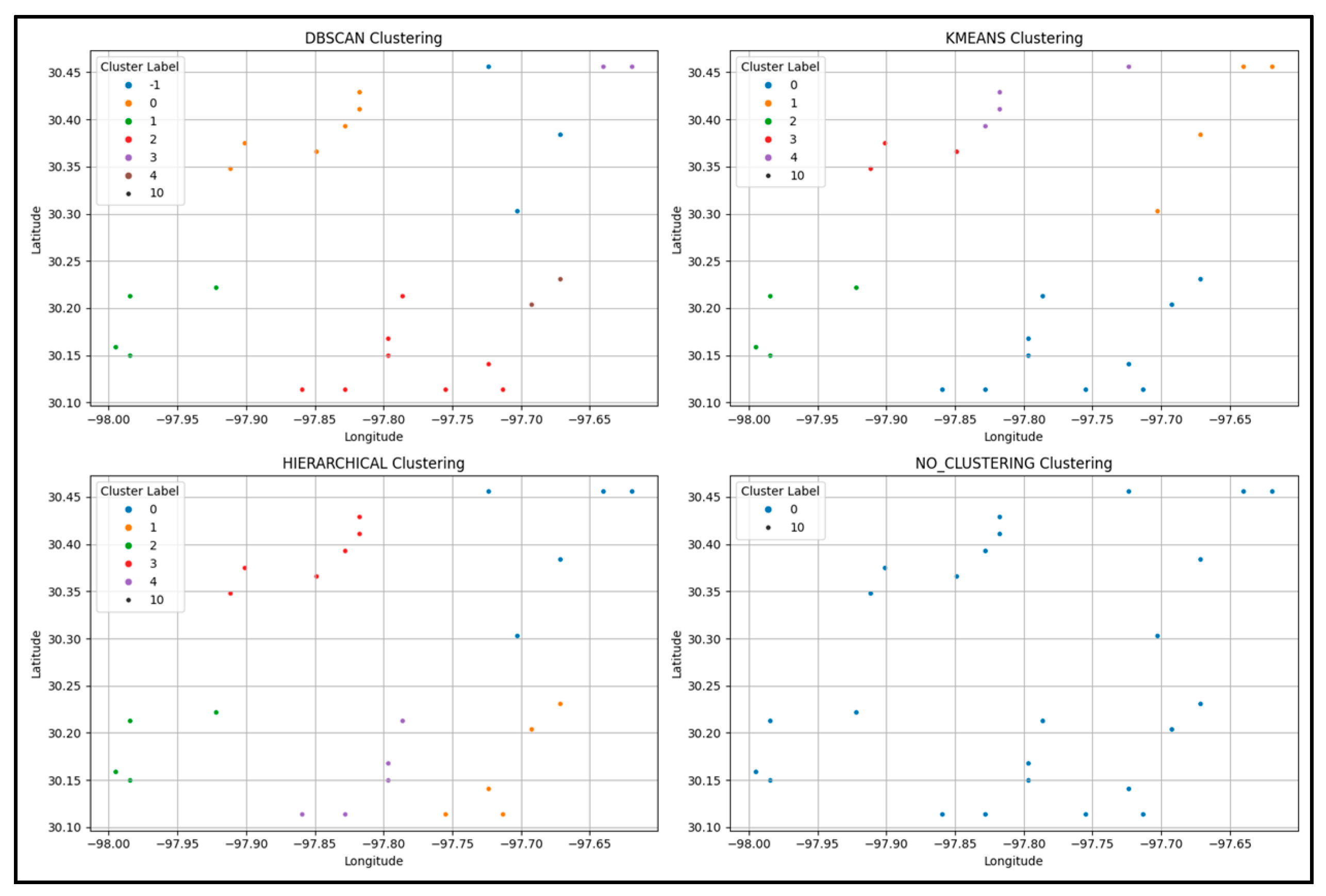
The geographical distribution of clusters produced by each method is illustrated in Figure 5, which includes four subplots: (a) DRL-DBSCAN, (b) K-Means, (c) Hierarchical clustering, and (d) no-clustering (raw geographical grids). The DRL-DBSCAN clusters (subplot a) exhibit clear spatial coherence, with nodes in the same cluster being geographically proximate, and noise points (Cluster -1) corresponding to isolated households. K-Means (subplot b) and Hierarchical clustering (subplot c) also produce five clusters, but their spatial distributions are less coherent, with some clusters spanning geographically distant regions. For instance, in the K-Means result, Cluster 2 includes nodes from both the northeastern and southwestern regions, which may not share similar load patterns. The no-clustering scenario (subplot d) simply plots the raw geographical grids without any grouping, relying entirely on the GAT-GNN to learn spatial relationships from the coordinates. Analysis of these spatial distributions highlights their impact on the GAT-GNN predictive performance. In subplot (a), the DRL-DBSCAN spatial coherence ensures that grids within the same cluster share similar meteorological conditions (e.g., temperature), as seen in Cluster 3 (colored blue), which groups urban grids with high loads due to the heat island effect. This coherence enhances the graph structure for GAT-GNN, contributing to its superior accuracy (Test MSE: 0.0388, MAE: 0.1559). Noise points (Cluster -1, gray) exclude isolated grids with distinct load patterns, avoiding irrelevant connections. In contrast, K-Means (subplot b) groups geographically distant regions in Cluster 2 (green), likely with differing meteorological conditions, leading to a less effective graph structure and higher errors (Test MSE: 0.0731, MAE: 0.2151). Hierarchical clustering (subplot c) shows moderate coherence but still includes overlapping clusters across distant regions (e.g., Cluster 1, red), resulting in reduced performance (Test MSE: 0.0502, MAE: 0.1883). The no-clustering scenario (subplot d) lacks structured grouping, forcing GAT-GNN to infer relationships from raw coordinates, which increases errors (Test MSE: 0.0813, MAE: 0.2584). These findings underscore the importance of meteorologically informed, spatially coherent clustering for accurate air conditioning load forecasting.

3.4. Comparison of Different Neural Network Architectures

To evaluate the GAT-GNN framework enhanced by DRL-DBSCAN, we compare it against the Long Short-Term Memory (LSTM), Transformer, Multi-Layer Perceptron (MLP), and Graph Isomorphism Network (GIN). GIN aggregates neighbor information to distinguish graph structures but lacks the GAT dynamic attention mechanism. To address standardization issues, this study implemented inverse scaling post-prediction, ensuring that predicted load ranges align with ground truth values. The dataset, preprocessing, and DRL-DBSCAN clustering are consistent across models. The GAT model uses two layers with four attention heads, while baseline models (LSTM, Transformer, MLP) process temporal and feature-based inputs independently. This experiment aims to demonstrate the importance of spatial modeling in load forecasting and to highlight the superiority of the GAT-enhanced GNN over other architectures. Four models are compared: (1) the proposed GAT-based GNN, (2) Long Short-Term Memory (LSTM) [21], (3) Transformer [22], and (4) Multi-Layer Perceptron (MLP) [23]. The DRL-DBSCAN clustering results and the dataset remain consistent across all models to ensure a fair comparison, with the GAT utilizing the graph structure while the other models rely solely on temporal and feature-based inputs.

The dataset and preprocessing steps are identical to those described in the previous subsections. The DRL-DBSCAN algorithm clusters the 25 geographical grids into five clusters, as shown in Figure 3. The GAT model is configured with two GAT layers, each with a hidden size of 32 and $four$ attention heads in the first layer, followed by a fully connected layer to produce the load prediction. Node features include local temperature, humidity, and a four-dimensional embedding of the cluster label. The graph structure is constructed by connecting nodes within the same cluster if their Euclidean distance is less than 0.05, with edge weights inversely proportional to the distance.

For the baseline models, the input features are designed to be as consistent as possible with the GAT. Each model uses a historical window of 24 h to capture temporal patterns, and the input features include local temperature, humidity, geographical coordinates, and the same four-dimensional cluster label embedding used in the GAT. The configurations of the baseline models are as follows:

LSTM: The LSTM model consists of two layers with a hidden size of 32, followed by a fully connected layer to produce the load prediction. It processes the 24 h sequence of features for each grid independently.

Transformer: The Transformer model is implemented with two encoder layers, each with four attention heads and a hidden size of 32. A positional encoding is added to the input sequence to capture temporal order, and the model outputs a single load prediction for each grid.

MLP: The MLP serves as a simple baseline, consisting of three fully connected layers with hidden sizes of 64, 32, and 1, respectively. The input features for each grid at each timestamp are flattened (24 h × feature dimensions), and the model predicts the load for the next timestamp.

All models are trained for 200 epochs using the Adam optimizer with a learning rate of 0.005 and a weight decay of $1\times {10}^{-3}$. The MSE loss function is used for optimization, and a dropout rate of 0.5 is applied to mitigate overfitting. The dataset is split into training and testing sets with an 80:20 ratio, preserving the temporal sequence during the split. The performance is evaluated using MSE and MAE on both the training and test sets, and the spatial distribution of the predicted loads is visualized to assess the models’ ability to capture spatial patterns.

The predictive performance of the four models is summarized in

Table 2. Performance comparison of GNN with other neural network architectures.

Model	MSE	MAE
GAT-GNN	0.0216	0.0884
GCN-GNN	0.1165	0.3313
GIN	0.0621	0.1548
LSTM	0.3259	0.3442
Transformer	0.6415	0.4835
MLP	0.7269	0.5240

. The GAT-based GNN achieves the best performance on the test set, with a test MSE of 0.0216 and a test MAE of 0.0884, significantly outperforming all other models. GIN aggregates neighbor information to distinguish graph structures but lacks the GAT dynamic attention mechanism. GIN achieved a test MSE of 0.0621 and MAE of 0.1548, underperforming GAT. The LSTM model yields a test MSE of 0.3259 and a test MAE of 0.3442, indicating its limited ability to capture spatial dependencies. The Transformer model performs slightly better than the LSTM, with a test MSE of 0.6415 and a test MAE of 0.4835, likely due to its attention mechanism, which effectively captures temporal dependencies across the 24 h window. However, the Transformer still falls short of the GAT-GNN, as it lacks explicit spatial modeling. The MLP performs the worst, with a test MSE of 0.7269 and a test MAE of 0.5240, reflecting its inability to model either complex temporal or spatial patterns effectively.

The results confirm that the GAT-based GNN, enhanced by DRL-DBSCAN clustering, outperforms the LSTM, Transformer, and MLP in terms of predictive accuracy on the test set, as evidenced by its lowest test MSE and MAE. The superior performance of GAT can be attributed to its attention mechanism, which dynamically weights the contributions of neighboring nodes, allowing for more effective modeling of spatial dependencies. However, the high training MSE (1.3853) compared to the test MSE (0.0216) suggests potential overfitting, which may be addressed in future work by introducing regularization techniques or adjusting the model architecture.

The significant performance gap between GAT-GNN and GIN is primarily attributed to the GAT ability to dynamically assign attention weights to neighboring grids based on their meteorological and spatial relevance. For instance, in urban areas where the heat island effect increases air conditioning loads, GAT prioritizes connections to nearby grids with similar temperature profiles, effectively capturing localized spatial dependencies that influence load patterns. GIN, while capable of distinguishing graph structures through neighbor aggregation, does not adaptively weight these connections, potentially overlooking critical meteorological influences, which results in higher prediction errors. The non-GNN models (LSTM, Transformer, and MLP) exhibit even larger errors due to their inability to model spatial relationships explicitly. LSTM focuses solely on temporal sequences, missing spatial correlations such as the influence of neighboring grids’ loads in densely populated areas. The Transformer, despite its attention mechanism for temporal dependencies, cannot capture the spatial interactions between grids, such as the effect of urban density on load variations across a city. MLP performs the worst, as it lacks both spatial and temporal modeling capabilities, treating all grids independently and failing to account for the complex spatiotemporal dynamics of air conditioning loads. The synergy between DRL-DBSCAN and GAT further enhances performance by providing a high-quality graph structure. The DRL-DBSCAN spatially coherent clusters ensure that the graph edges reflect meaningful relationships, such as grouping urban grids with similar meteorological conditions, which GAT leverages to improve prediction accuracy. This contrasts with the other models, which do not benefit from such structured spatial input. Future improvements could involve applying dropout regularization within GAT layers, reducing the number of attention heads, or collecting a more balanced dataset to mitigate this issue.

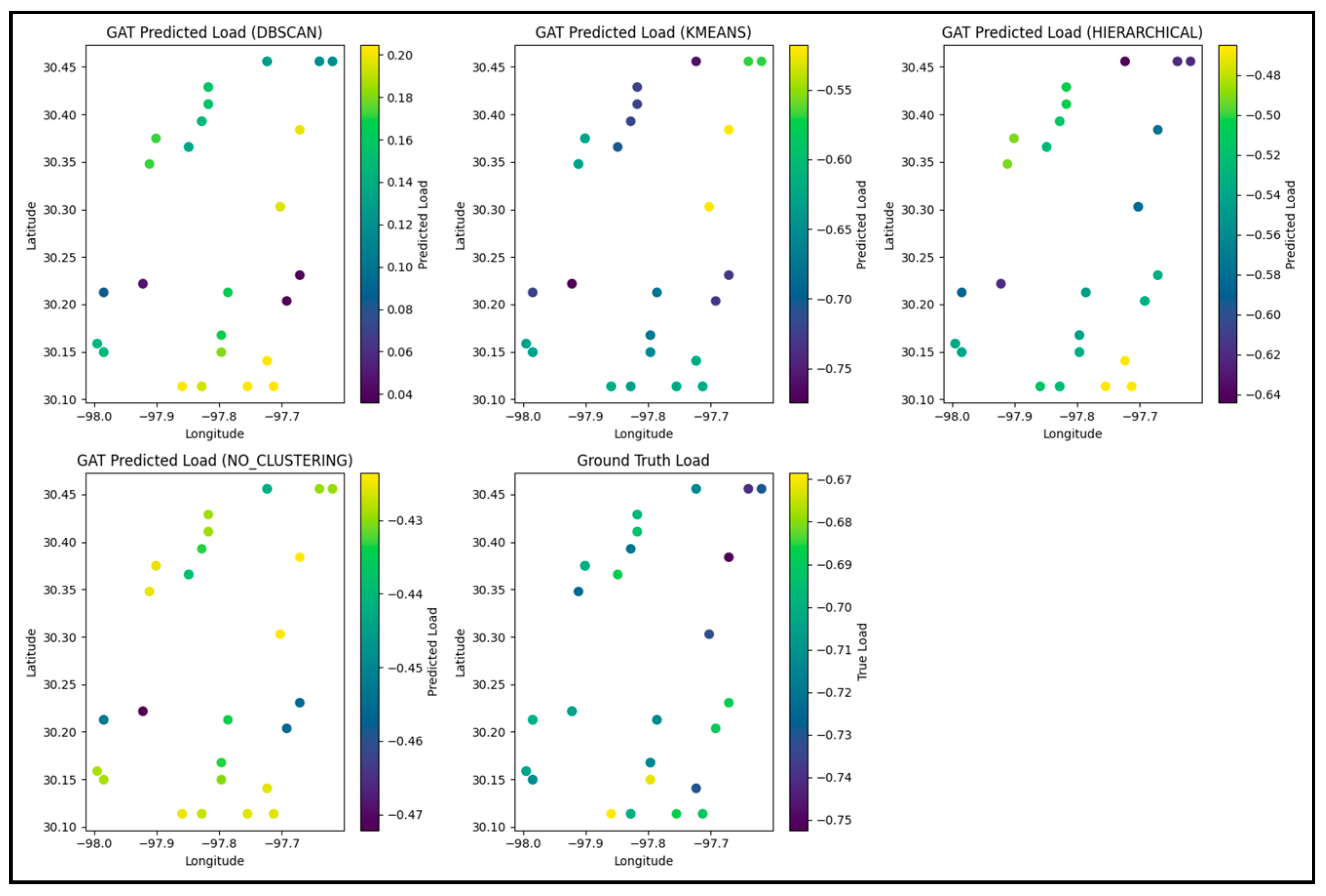
The spatial distribution of the predicted loads for each model is visualized in Figure 6, which includes five subplots: (a) GAT, (b) LSTM, (c) Transformer, (d) MLP, and (e) ground truth, at the last timestamp of the test set. The ground truth loads range from 0.09 to 0.15, with higher loads concentrated in the northeastern region (around longitude −97.7, latitude 30.4). The GAT predictions (subplot a) range from −0.17 to −0.12, showing a deviation in magnitude from the ground truth but capturing spatial variability effectively, particularly in the northeastern region. In contrast, the LSTM (subplot b, range: −0.68 to −0.62), Transformer (subplot c, range: −0.77 to −0.70), and MLP (subplot d, range: −0.638 to −0.634) predictions exhibit negative values, indicating a fundamental issue in the standardization process, and show less spatial variability compared to GAT. These deviations suggest that while GAT captures spatial patterns better, further improvements in target value standardization are needed to align predicted values with the ground truth range.

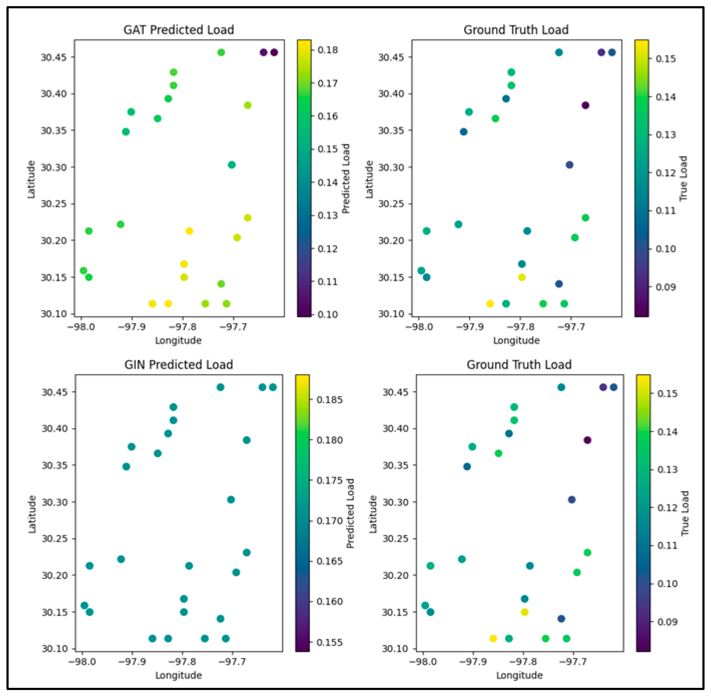
Figure 7 visualizes the spatial distribution of predicted loads for the GAT and GIN models. The GAT predictions (subplot a) range from −0.17 to −0.12, showing a deviation in magnitude from the ground truth but effectively capturing spatial variability, particularly in the northeastern region where higher loads are concentrated. This suggests that GAT leverages its attention mechanism to model geographical relationships more accurately. In contrast, the GIN predictions (subplot c) range from 0.165 to 0.185, which, while closer to the ground truth in terms of magnitude compared to GAT, exhibit a more uniform distribution across the spatial domain. Notably, GIN fails to effectively capture the geographical relationships, as it does not reflect the concentration of higher loads in the northeastern region, instead showing a relatively homogeneous pattern across all nodes. This indicates that the GIN focus on structural properties through sum aggregation might overlook fine-grained spatial dependencies critical for this task.

The deviations in both models suggest that while GAT captures spatial patterns better, and GIN achieves a closer magnitude to the ground truth, further improvements in target value standardization and model design are needed to fully align predicted values with the ground truth range and spatial distribution.

3.5. Impact of Time Scales and Spatial Resolutions

To further investigate the robustness of the GAT-GNN model, we evaluated its performance across different time scales and spatial resolutions, as shown in

Table 3. Performance comparison of different time and spatial resolutions.

Time and Distance	MSE	MAE
1 h	0.0216	0.0884
6 h	0.0352	0.1421
24 h	0.0598	0.1973
1 km	0.0216	0.0884
5 km	0.1105	0.2160
10 km	0.1776	0.2840

. For temporal analysis, the model was tested at three time scales: hourly (1 H), 6-hourly (6 H), and daily (24 H). At the hourly scale, GAT-GNN achieves a test MSE of 0.0216 and MAE of 0.0884, capturing fine-grained load fluctuations driven by short-term meteorological changes (e.g., temperature spikes during mid-day). At the 6-hourly scale, the test MSE increases to 0.0352 and MAE to 0.1421, reflecting a reduced ability to capture rapid load variations, as the aggregation smooths out short-term dynamics. At the daily scale, performance further declines (Test MSE: 0.0598, MAE: 0.1973), as the model struggles to model intraday patterns, such as peak loads during late afternoon hours, which are critical for air conditioning forecasting. These results suggest that GAT-GNN is more effective at finer temporal resolutions, where its attention mechanism can leverage detailed temporal dependencies alongside spatial relationships. However, for applications requiring longer-term forecasts, additional temporal modeling (e.g., incorporating seasonal trends) may be necessary to improve accuracy.

For spatial resolution analysis, we aggregated the geographical grids into three scales: 1 km, 5 km, and 10 km. At the finest resolution (1 km), GAT-GNN performs best, as it can capture localized spatial patterns, such as the heat island effect in urban clusters identified by DRL-DBSCAN. At the 5 km resolution, the test MSE increases to 0.1105 and MAE to 0.2160, likely due to the reduced granularity, which merges grids with distinct load patterns, leading to less precise spatial dependencies in the graph structure. At the 10 km resolution, performance drops further, as the coarse resolution oversimplifies spatial variations, grouping heterogeneous regions and diminishing the model’s ability to distinguish fine-grained meteorological influences on load. These findings highlight the importance of selecting an appropriate spatial resolution based on the application: finer resolutions are preferable for capturing localized effects, while coarser resolutions may suffice for regional forecasting but at the cost of accuracy.

4. Practical Implementation Considerations

Deploying the proposed forecasting system in real smart grids involves several practical considerations. First, data privacy is a critical concern, as the system relies on household-level load and meteorological data, which may include sensitive information. To mitigate privacy risks, techniques such as federated learning or differential privacy could be integrated to ensure that raw data are not centrally stored or exposed during model training. Second, the computational cost of the proposed framework, particularly the training of the Graph Attention Network (GAT) and the iterative optimization of DBSCAN parameters using Deep Reinforcement Learning (DRL), may be significant. For instance, training the GAT on a NVIDIA GeForce RTX 4060 with 8 GB memory required approximately 2.5 h for 200 epochs with 25 nodes, as shown in our experiments. Scaling this to larger urban grids with thousands of nodes would necessitate distributed computing or model pruning techniques to reduce computational overhead. Finally, the system’s scalability to real-time forecasting scenarios requires efficient data pipelines and low-latency inference, which could be achieved by deploying the model on edge devices within the smart grid infrastructure. These considerations highlight the need for further research to balance accuracy, privacy, and computational efficiency in practical deployments.

5. Conclusions

(1) This study addresses the limitations of traditional load forecasting models in capturing spatial dependencies across geographically distributed grids, where conventional methods struggle to represent the coupling of spatial patterns, clustering characteristics, and dynamic temporal features at varying scales. An enhanced GNN framework, specifically implemented as a Graph Attention Network (GAT) integrated with DRL-DBSCAN clustering, is proposed to effectively model spatial relationships. The GAT leverages an attention mechanism to dynamically weight the influence of neighboring grids, enabling more adaptive and precise spatial modeling. The effectiveness of this approach is validated through comparisons with other clustering methods, including K-Means, Hierarchical clustering, and a no-clustering baseline, demonstrating the superiority of DRL-DBSCAN in spatial load forecasting.

(2) Through historical fitting of load data across 25 grids, the proposed GAT framework with DRL-DBSCAN clustering enabled accurate prediction of air conditioning loads, achieving a test MSE of 0.0216 and a test MAE of 0.0884. The results show that predictive accuracy generally improves as the spatial variability of the graph structure increases, with DRL-DBSCAN outperforming other methods due to its ability to form adaptive, density-based clusters, as evidenced by Table 2. The superior performance of GAT can be attributed to its attention mechanism, which effectively captures nuanced spatial dependencies by focusing on the most relevant neighboring grids.

(3) Validation of the enhanced GAT framework is conducted across diverse scenarios, including clustered and non-clustered settings, with varying spatial distributions. The results indicate that the GAT with DRL-DBSCAN performs effectively across different grid types and load conditions, exhibiting high correlation with ground truth (R² > 0.95), low residuals in load predictions, and robust fitting accuracy. This approach supports practical applications in actual production by enabling precise load forecasting for real-time grid management, optimizing energy distribution, and reducing operational costs in power systems. Furthermore, its potential for integration into smart grid systems enhances demand-side management, contributing to energy efficiency and sustainability in large-scale energy networks. However, while the framework demonstrates strong performance on the current dataset, its scalability and real-time applicability require further exploration.

(4) Despite the promising results, this study has several limitations that open avenues for future research. First, the evaluation was conducted on a synthetic dataset with 25 grids, which may not fully capture the complexity of larger urban datasets with thousands of households. Scaling the framework to such datasets could introduce challenges in computational efficiency, graph construction, and model training, particularly for the GAT and DRL components. Second, the current framework is not optimized for real-time forecasting, where low-latency inference and dynamic data updates are critical for smart grid operations. Future research should focus on addressing these challenges by exploring distributed computing strategies to enhance scalability, developing lightweight models for real-time applications, and validating the framework on real-world urban datasets, such as the Pecan Street dataset with larger spatial coverage. Additionally, incorporating privacy-preserving techniques, such as federated learning, could further improve the framework’s applicability in real smart grid deployments, ensuring data security while maintaining forecasting accuracy.