Abstract
As global energy grows short and environmental governance pressure increases, the automotive industry, a major energy consumer and pollution emitter, must enhance vehicle aerodynamics to cut energy use and emissions. This study creates an open-domain and virtual wind tunnel dual-computational-domain setup. It optimizes mesh refinement and boundary conditions, and evaluates the k-ε, k-ω, and Detached Eddy Simulation (DES) turbulence models. These models predict vehicle aerodynamic resistance, lift, and wake flow structure. The k-ε model best predicts the steady-state drag coefficient (Cd) (error 0.0009). DES excels in transient conditions (Cd error −0.4%, lift coefficient Cl matching experiments). The k-ω model, with its near-wall flow capture ability, has the lowest lift prediction error (−2.7%). Moreover, open-domain simulations align more closely with real free-flow environments and experimental data than virtual wind tunnel simulations. Overall, the study clarifies the varying applicability of turbulence models in complex flows, and offers a basis for model selection and technical support for vehicle aerodynamic optimization. It is highly significant for reducing fuel consumption, boosting the range of new-energy vehicles, and promoting sustainable industry development.
1. Introduction
1.1. Research Background
With increasing global energy demands and environmental concerns, the automotive industry, as a major energy consumer and pollutant emitter, plays a crucial role in energy conservation and emission reduction. During the process of vehicle operation, air resistance, as one of the key factors affecting fuel consumption and exhaust emissions, has a significant effect on energy saving and emission reduction. Statistics show that the aerodynamic resistance of a car is directly proportional to the square of its speed. When the speed reaches 60 km/h, the impact of aerodynamic resistance on driving becomes very obvious, and it is almost equivalent to rolling resistance; while when the speed exceeds 120 km/h, aerodynamic resistance will become the main component of the total resistance of the car, equivalent to 2 to 3 times the rolling resistance [1]. The higher the speed, the greater the proportion of air resistance. Previous studies have shown that for every 10% decrease in the vehicle resistance coefficient, energy consumption can be reduced by 3.5 to 8%. For electric vehicles, a 0.02 decrease in the vehicle resistance coefficient can increase the range by more than 10 km. Therefore, in recent years, automotive enterprises in various countries have gradually increased their research and development investment in the field of reducing vehicle resistance. With the continuous application of new resistance reduction technologies, the future development of automotive aerodynamics will further significantly reduce energy consumption [2].
1.2. Research Status
Currently, vehicle aerodynamics research mainly adopts wind tunnel experiments and computational fluid dynamics (CFD) simulation as two main methods. Wind tunnel experiments, as a traditional research method, have advantages such as intuitiveness and accuracy, which can truly simulate the airflow environment during vehicle driving and obtain key data such as pressure distribution and aerodynamic forces on the vehicle surface [3]. In the wind tunnel test, the vehicle wake interaction was studied, accurately capturing the impact of the complex vortex structures behind the vehicle on the aerodynamic performance of trailing vehicles [4]. However, wind tunnel experiments also have some limitations, such as high experimental costs, long periods, and difficulty in simulating complex real road conditions due to experimental conditions [5]. For example, constructing a large-scale automotive wind tunnel requires substantial investment, and each experiment consumes a large amount of manpower, material resources, and time. In addition, the boundary conditions in wind tunnel experiments are difficult to be completely consistent with actual road driving conditions, which may lead to certain deviations between the experimental results and actual operating conditions. In Guerrero’s underbody flow study, wind tunnel tests were found to have discrepancies in simulating the complex airflow under vehicles compared to real road conditions [6].
CFD Simulation Technology as a new research method has the advantages of low cost, high flexibility, and the ability to deeply analyze the details of the flow field. By establishing a vehicle geometric model and using numerical methods to solve fluid mechanics equations, it is possible to simulate the flow field distribution around the vehicle and predict aerodynamic parameters such as air resistance, lift, and lateral force [7]. In studies by Cravero and Fernandez-Gamiz, they used CFD simulations to deeply explore wheel aerodynamics, analyzing how the vortices from wheel rotation–airflow interactions affect whole-vehicle aerodynamic performance [8,9].
However, CFD simulation also faces some challenges, such as grid quality, turbulence model selection, and boundary condition settings, which can affect the accuracy of the simulation results [10]. For example, unreasonable grid division may lead to insufficient calculation accuracy or high calculation cost, an inaccurate turbulence model may fail to accurately predict complex turbulence phenomena, and improper boundary condition settings may cause the simulation results to deviate from the actual working conditions. Therefore, how to improve the accuracy of CFD simulation and make it better serve the optimization of vehicle aerodynamics is an important research topic at present.
1.3. Research Objectives
Considering the advantages and disadvantages of wind tunnel experiments and CFD simulations, this study aims to explore the role of virtual wind tunnel simulation technology in improving the prediction accuracy of vehicle aerodynamics. The virtual wind tunnel simulation combines the authenticity of wind tunnel experiments with the flexibility of CFD simulations, and by simulating the actual structure and working conditions of wind tunnels, it can to some extent overcome issues such as inaccurate boundary condition settings and unrealistic flow field simulation in traditional CFD simulations, thereby improving the reliability of simulation results. This study will delve into the accuracy and advantages of virtual wind tunnel simulation analysis of vehicle aerodynamic performance in predicting vehicle air resistance, pressure distribution, and tail flow field structure, providing more efficient and accurate technical support for vehicle aerodynamic optimization, helping the automotive industry achieve energy conservation and emission reduction goals, and promoting the sustainable development of the automotive industry.
2. Methods and Models
2.1. Computational Domain Setup
1. Open Domain: A rectangular space (60 m × 17.5 m × 10.5 m) simulating real-world driving conditions, ensuring minimal interference with airflow calculations. This design avoids unnecessary interference to the flow field caused by a small computational domain, ensuring the accuracy and completeness of flow field calculations. The structure and dimensions of the open domain are shown in Figure 1.

Figure 1.
Open-domain structure diagram.
2. Virtual Wind Tunnel: Accurately replicates the actual wind tunnel structure, including the contraction section, nozzle, and intake, etc. The contraction section accelerates the airflow, the nozzle precisely controls the speed and direction of the airflow, and the intake stabilizes the airflow, reducing vortex interference, creating a realistic wind tunnel environment for the vehicle model, and ensuring the reliability of the simulation results. The structure and dimensions of the wind tunnel are shown in Figure 2.

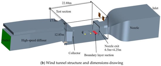
Figure 2.
Wind tunnel structure diagram.
2.2. Mesh Strategy
The research on grid independence refers to the findings of Liao G et al. [11] The open domain and virtual wind tunnel use the same mesh strategy as shown in Table 1 and structure of the three-level encryption domain as shown in Figure 3. The encrypted separation area and near-wall area: Grid densification is performed in areas prone to flow separation and significant boundary layer effects, such as the vehicle’s rear and bottom, to capture fine flow field characteristics such as flow separation and boundary layer thickness changes, providing a foundation for accurate calculation of air resistance and pressure distribution.

Table 1.
Encryption domain settings.
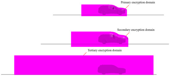
Figure 3.
Structure of the three-level encryption domain.
Optimization Y+ value: Controlling the Y+ value within the range of 30–100, balancing grid accuracy and computational cost, both excessively high or low Y+ values will affect the accuracy and convergence of the turbulence model, and reasonable optimization of the Y+ value can improve the accuracy of turbulence simulation [12].
2.3. Transient Simulation Conditions
The time step invariance of this study is based on the research results of Liao G et al. [11]. It adopts an implicit unsteady solution, with a time step of 0.001 s, a maximum physical time of 10 s, and a maximum internal iteration of 5.
2.4. Boundary Conditions
1. Open Domain:
(1) The inlet is set as a velocity inlet: Set to 120 km/h and 140 km/h, simulating the incoming flow velocity during high-speed vehicle driving. The aerodynamic performance of the vehicle varies under different speeds, and the air resistance increases significantly at high speeds. Accurately simulating the velocity inlet is crucial for predicting the actual driving state of the vehicle.
(2) Set the outlet as a pressure outlet: Set to 0 Pa, maintain pressure balance within the computational domain, ensure smooth flow out of the airflow, and avoid pressure fluctuations causing errors in the flow field calculation, ensuring the stability and accuracy of the outlet flow field.
(3) Simulation of Moving Ground and Rotating Wheel: Using moving ground to simulate the vehicle’s relative motion to the ground during driving, the rotating wheel wall and hub moving reference frame (MRF) simulates the wheel rotation, realistically reproducing the vehicle driving conditions, considering the interaction between the vehicle and the ground, and the wheel and air, to enhance the credibility of the simulation results.
2. Virtual Wind Tunnel:
The inlet is set as a mass flow inlet, and the outlet is set as a mass flow outlet. Stable section: The inlet uses a mass flow inlet, the first-stage exhaust outlet uses a pressure outlet, the second-stage suction outlet uses a velocity outlet, and the third-stage energy supplement uses a velocity inlet. Stationary chamber section: The outlet uses a pressure outlet, the flow supplement on both sides of the gas collection port uses a mass flow inlet, and the diffuser section outlet uses a mass flow outlet. Tangential velocity and no-slip conditions are used to simulate the five-zone system, and the wheel rotation wall and hub moving reference frame are used to simulate wheel rotation.
2.5. Numerical Methods and Software Implementation
The three control equations of fluid dynamics are solved using numerical calculation methods [13].
The mass conservation equation, also known as the continuity equation, describes the change in mass within the fluid, and states that the rate of change in mass per unit volume is equal to the sum of the mass fluxes flowing into and out of the unit volume. That is,
In the equation, ρ represents the density of the fluid, usually expressed in units of kilograms per cubic meter (kg/m3). t represents time, usually in seconds (s). v represents the velocity vector field of the fluid, which includes the velocity components of the fluid in the three spatial directions, usually in meters per second (m/s). ∇ represents the gradient operator, used to describe the gradient of the vector field.
The momentum equation describes the change in momentum within a fluid. The left side of the equation represents the rate of change in momentum per unit volume, while the right side consists of the pressure gradient force, viscous stress, and volume force. That is,
In the equation, p represents the pressure of the fluid, and the unit is usually pascal (Pa). τ represents the viscous stress tensor, which describes the viscous effect within the fluid. It represents the volume force vector field, including the external volume forces acting on the fluid, such as gravity, etc.
The energy equation describes the change in energy within the fluid. The left side of the equation represents the rate of change in energy per unit volume, and the right side consists of pressure power, viscous power, heat transfer power, and power density. That is
In the equation, e represents the total energy per unit mass of the fluid, which includes internal energy, kinetic energy and potential energy, etc. q represents the heat flux vector, which describes the heat transfer process within the fluid. These three equations are the basic equations for describing fluid motion, and together they form the foundation of fluid dynamics.
The accurate and timely prediction of the airflow separation on the smooth surface of the car is important in the computational simulation of the automobile’s external flow field. Thus, the selection of a turbulence model is relatively demanding. For comparative analysis, this study selects three numerical simulation methods, namely, realizable K-Epsilon, SST K-Omega, and SST DES, which are commonly used in automotive simulation, to establish a numerical wind tunnel simulation model with a good fit to the actual wind tunnel experimental values.
As the most widely used turbulence model in the solution of automobile winding problems, the steady-state k-ε two-equation model is a high-Reynolds-number model derived under fully developed turbulent flow conditions and is suitable for regions with sufficiently large turbulent Reynolds numbers. The automobile turbulent flow field calculation involves the wall and the boundary layer covering the wall. The viscous bottom layer and the transition zone exist near the wall. The turbulent Reynolds number is very small, and the Reynolds stress and molecular viscous stress are of the same order of magnitude. The calculation must consider the effect of molecular viscosity.
Therefore, the realizable k-ε turbulence model is chosen, which has new turbulence control equations and transfer equations for the dissipation rate. It is also capable of highly accurate predictions in complex flows involving rotations, boundary layer separations under strong backpressure gradients, and reflux. Moreover, it is highly suitable for designing the automotive flow field in walled boundary layers for simulation [14].
The steady-state k-ω two-equation turbulence model allows the transport equations for turbulent kinetic energy k and unit dissipation rate ω to be solved, thereby determining the aerodynamic coefficients without involving complex nonlinear decay functions like those required in the k-ε model. The SST k-ω turbulence model combines the advantages of the K-Epsilon turbulence model, which performs well in the region outside the boundary layer, and the K-Omega model, which is suitable for the near-wall treatment of the low Reynolds number case. Thus, the SST k-ω turbulence model can accurately predict the incoming flows and accurately simulate the separation phenomena under various pressure gradients. It also has advantages in the simulation of automotive flow fields. However, the two turbulence models are time averaged. Thus, the features of various sizes of vortices are erased, thereby failing to reflect the real vortex shedding phenomenon.
DES methods are common for hybrid RANS/LES models. Spalart [15] proposed a DES method based on the SST model. The SST DES turbulence model introduces DES features to reduce turbulence viscosity, thereby realizing a smooth transition from RANS to LES with a sufficiently fine mesh. Combining the advantages of RANS and LES provides high accuracy and efficiency in complex flow simulations. Moreover, this combination is suitable for flow fields that require transient analysis.
This study employs a numerical discretization scheme based on the Finite Volume Method (FVM) and uses the commercial CFD software Siemens STAR-CCM+ 15.02.007-R8 for the solution. The specific numerical scheme is as follows: Spatial discretization: The convection term uses the second-order upwind scheme to accurately capture the flow gradient and turbulence characteristics; the diffusion term uses the central difference scheme to ensure the numerical stability of the viscous term; gradient reconstruction is based on the least squares method to ensure the second-order accuracy of spatial derivatives. Time discretization: Steady-state simulations use the implicit time integration scheme (Implicit Time Stepping) to converge to the steady-state solution through pseudo-time stepping; transient simulations use the second-order implicit scheme (Second-Order Implicit Scheme), and the time step is adjusted adaptively according to the local Courant number (Co < 1) to ensure the second-order accuracy in the time direction. Pressure–velocity coupling: The SIMPLE algorithm (Semi-Implicit Method for Pressure-Linked Equations) is used to iteratively correct the pressure field and velocity field to balance the mass conservation and momentum conservation equations.
STAR-CCM+ defaults to a second-order accuracy spatial discretization, and the transient time discretization also satisfies second-order accuracy. This setting has been verified through classic examples (such as the flow around the NACA 0012 airfoil and Ahmed vehicle wake simulation) and is consistent with the theoretical benchmark results in reference [16] and the software technical documentation [17].
3. Experiment and Data Collection
3.1. Experimental Platform
Using a full-scale aerodynamic acoustic wind tunnel (AAWT), equipped with a five-belt balancing system and boundary layer control systems (BLCs). The five-belt balancing system can accurately measure the aerodynamic forces and torques of the vehicle under different driving attitudes, and the boundary layer control systems effectively control the thickness of the boundary layer inside the wind tunnel, reducing the interference of the boundary layer on the experimental results, ensuring the accuracy and reliability of the experimental data [18].
The wind speed was measured using a hot-wire anemometer (HWA, Dantec 55P11, Copenhagen, Denmark) at the centerline position of the test section (5 m from the inlet), with a sampling frequency of 10 kHz and a duration of 60 s. The measured values were TI = 0.42% ± 0.05% (at 120 km/h condition) and TI = 0.38% ± 0.04% (at 140 km/h condition), which met the wind tunnel design specifications (TI < 0.5%).
3.2. Pressure Data Acquisition Instrument
In this study, the Basic Instrument, Model CPG2500 (WIKA Alexander Wiegand SE & Co. KG, Frankfurt, Germany) was used for pressure measurement. This sensor has a measurement range of −0.18 to −0.18 to −14.5 to 15,000 psi. When the measurement range is ≤15 psi, only pneumatic media can be used; when the measurement range is >15 psi, both pneumatic and non-corrosive hydraulic media can be used. The accuracy is 0.004% FS. From its high precision and various pressure unit outputs, it can be widely applied in industrial automation, medical equipment, automotive electronics, and other fields, providing precise pressure data support for various pressure measurement and control systems.
3.3. Data Collection
As shown in Figure 4, ten surface pressure measurement points are set at the vehicle rear to comprehensively collect vehicle surface pressure distribution data, analyze the pressure change law, accurately measure the rear vortex structure and velocity field information, deeply explore the rear flow field characteristics, and provide key data support for optimizing the vehicle’s rear aerodynamic performance [19].

Figure 4.
Pressure measurement point distribution map.
4. Results and Discussion
We conducted open-domain simulations at 140 km/h steady-state and 120 km/h transient open-domain, compared the lift, drag values, and tail pressure values at 10 pressure measurement points of the simulation results with the test data, and explored the advantages and disadvantages of different simulation models.
The reason this article uses a 140 km/h steady-state model for simulation and a 120 km/h transient model for simulation is rooted in the nature of the flow conditions and the goals of accuracy and realism in aerodynamic prediction.
At 140 km/h, the vehicle is considered to be in a high-speed, steady-state driving condition, meaning the airflow around the vehicle is relatively stable, and the focus is on understanding the aerodynamic performance under a constant speed scenario, which simplifies the simulation and makes it easier to match with wind tunnel test data.
At 120 km/h, the study switches to a transient model because, at lower speeds, the airflow is more prone to dynamic effects like separation, vortex shedding, and unsteady wake behavior. A transient simulation allows the model to capture these time-dependent flow changes, which are especially relevant when the vehicle is in conditions where speed fluctuations, turbulence, or unsteady flow structures play a bigger role.
The paper also discusses how the DES model (which is better for transient flows) showed improved accuracy at 120 km/h, highlighting why the transient approach was necessary at that speed.
This study selects the k-ε, k-ω, and DES (Detached Eddy Simulation) turbulence models, respectively, simulating the aerodynamic performance of the Hong qi HS7 model at 120 km/h and 140 km/h conditions, and comparing them with wind tunnel experimental data. The comparison of steady-state operating conditions results is as shown in Table 2.

Table 2.
Comparison of steady-state operating conditions results.
The drag coefficient of the k-ε model deviates significantly from the experimental values, which may be due to its insufficient prediction of separated flow. The k-ω model performs optimally in lift prediction, with an error of only −2.7%, thanks to its fine capture of near-wall flow. The DES model has the smallest error in drag prediction ( +0.3%), indicating that its transient capability still has an advantage in steady-state simulations.
An analysis of the results in Table 3 reveals that the DES model significantly reduces error under transient conditions, with drag coefficient error as low as −0.4%, and lift coefficient perfectly matching the experimental values, verifying its advantage in dynamic flow fields. The k-ε model error increases, indicating its difficulty in capturing the complex structure of transient separation vortices.

Table 3.
Comparison of results for transient operating conditions.
Simulation values vs. experimental values: It can be seen from the Figure 5 that in the 120 km/h transient simulation, there is a significant difference in the pressure coefficients at each pressure measurement point between the simulation values (blue) and the experimental values (orange). The pressure coefficients from point 1 to 10 are generally lower than the experimental values, especially at points 1, 2, 3, 4, 5, 6, 7, 8, 9, and 10, where the difference between the simulation values and the experimental values is relatively obvious. For example, the simulation value at point 1 is about −0.12, while the experimental value is about −0.08; the simulation value at point 10 is about −0.04, while the experimental value is about −0.02.
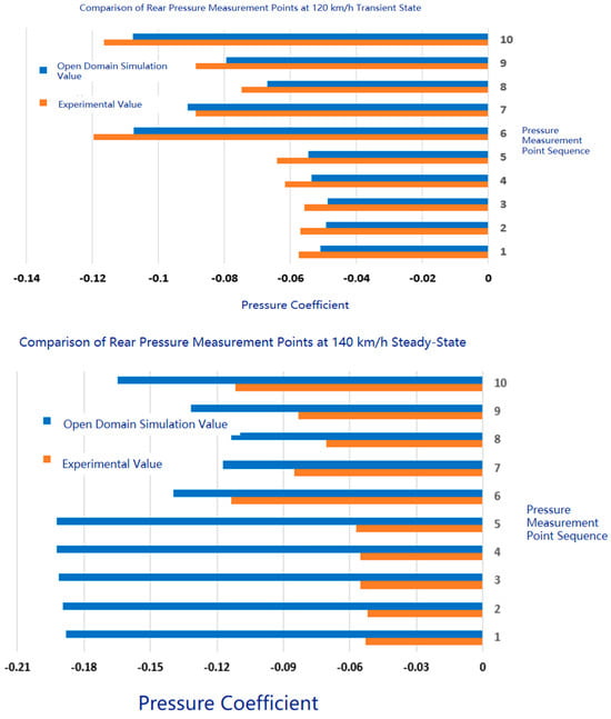
Figure 5.
Comparison of tail pressure points.
Simulation values vs. experimental values: It can be seen from the figure that in the steady-state simulation at 140 km/h, the pressure coefficient difference between the simulation values (blue) and the experimental values (orange) at each pressure measurement point is relatively small. The pressure coefficients at pressure measurement points 1 to 10 are relatively close between the simulation values and the experimental values, especially at points 1, 2, 3, 4, 5, 6, 7, 8, 9, and 10, where the difference between the simulation values and the experimental values is small. For example, the simulation value at pressure measurement point 1 is about −0.18, while the experimental value is about −0.16; the simulation value at pressure measurement point 10 is about −0.03, while the experimental value is about −0.02.
In the transient simulation at 120 km/h, the difference between the simulation values and the experimental values is significant. This may be due to the fact that transient simulation needs to consider more dynamic factors, such as vehicle acceleration, deceleration, and air flow instability, which are difficult to fully capture in the simulation, leading to a significant deviation between the simulation results and the actual experimental values. In the steady-state simulation at 140 km/h, the difference between the simulation values and the experimental values is smaller. Steady-state simulation assumes that the vehicle is traveling at a constant speed, with relatively stable air flow, so the simulation results are closer to the actual experimental values.
Transient Simulation Model: There may be certain limitations in the transient simulation model when capturing dynamic changes, especially at low speeds (120 km/h), where the model may not fully simulate the actual airflow changes, resulting in a significant deviation between the simulation results and the experimental values. Steady-state Simulation Model: The steady-state simulation model performs well in simulating the airflow distribution at a constant speed, with the simulation results being relatively close to the experimental values, indicating that the model has a high accuracy under steady-state conditions.
In the transient simulation at 120 km/h, there is a significant deviation between the simulation results and the experimental values, indicating that the transient simulation model has a lower accuracy in capturing dynamic changes. To improve the accuracy of the transient simulation, it is considered to introduce more complex dynamic models, such as considering the acceleration, deceleration of the vehicle, and the turbulent characteristics of the airflow, to better simulate the actual working conditions. In the steady-state simulation at 140 km/h, the simulation results are relatively close to the experimental values, showing that the steady-state simulation model has a higher accuracy in simulating the airflow distribution under constant speed. The steady-state simulation model performs well under the current working conditions, and the model parameters can be further optimized to further improve the accuracy of the simulation results.
We compared the lift and drag values of the k-ε, k-ω, and open-domain steady-state k-ε models of the numerical wind tunnel under steady-state simulation conditions with the results of the numerical wind tunnel simulation of the steady-state wind tunnel.
The horizontal axis of Figure 6 is the number of iterations, ranging from 0 to 8000, and the vertical axis is the drag coefficient Cd, with a range of approximately 0.25 to 0.55. The curve fluctuates greatly at first, especially within the first 1000 iterations, where the Cd value rapidly rises from around 0.25 to around 0.5, then gradually decreases and stabilizes, finally settling around 0.35.
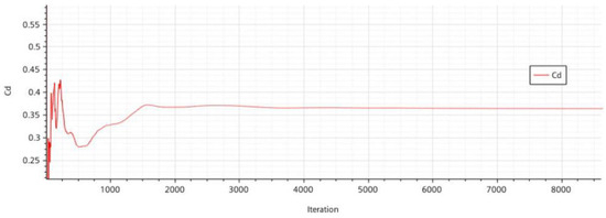
Figure 6.
k-ε model wind speed 140 km/h steady-state results.
The horizontal axis of Figure 7 is also the number of iterations, ranging from 0 to 7000, and the vertical axis is the drag coefficient Cd, with a range of 0.2 to 0.6. The curve also has a significant fluctuation at the beginning, but it is slightly smaller than that in Figure 6. The Cd value starts from around 0.2 and quickly rises to around 0.4, then gradually decreases and stabilizes, finally settling around 0.4.
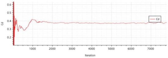
Figure 7.
K-ω wind speed 140 km/h steady-state results.
Initial Fluctuations: The initial fluctuation amplitude in Figure 6 is larger, which may be due to the insufficient stability of the k-e model in the initial stage for turbulent flow. Convergence Speed: Figure 6 tends to stabilize after about 2000 iterations, while Figure 7 becomes relatively stable after about 1000 iterations, indicating that the turbulent model used in Figure 7 has a faster convergence speed. Final Drag Coefficient: Figure 6 stabilizes at around 0.35, while Figure 7 stabilizes at around 0.4, although the difference between the two is not significant, but the drag coefficient of Figure 7 is slightly higher. Model Differences: The k-e model performs better at high Reynolds numbers, but may not be accurate in certain cases for low Reynolds numbers or near-wall regions. The k-ω model usually performs better in near-wall regions and may be more suitable for certain specific flow conditions.
These differences may be related to the applicability range and calculation accuracy of the turbulence model. Different turbulence models may have different performances when dealing with complex flow phenomena. Therefore, when selecting a turbulence model, it is necessary to decide according to the specific flow conditions and calculation requirements.
Finally, these two figures show the variation in drag coefficients under different turbulence models in the steady-state analysis at 140 km/h. Figure 6 uses the k-e model, with initial fluctuations being larger and convergence slightly slower, and the final drag coefficient being approximately 0.35. Figure 7 uses another turbulence model, with initial fluctuations being smaller and convergence faster, and the final drag coefficient being approximately 0.4. These differences indicate that choosing the appropriate turbulence model is very important for accurately predicting drag coefficients.
An analysis of the results in Table 4 reveals that for the comparison test value 0.3608, the simulation value of the numerical wind tunnel steady-state k-ε is the closest, with an error of 0.0028. The simulation value of the numerical wind tunnel steady-state k-ω has an error of 0.0136. The simulation value of the open field steady-state k-ε has an error of 0.0009, which is slightly better than the numerical wind tunnel steady-state k-ε.

Table 4.
Comparison of simulation results and accuracy of three simulation conditions.
Open-domain steady-state k-ε has the highest accuracy, close to 100%. Numerical wind tunnel steady-state k-ε also has high accuracy, 99.22%, while the accuracy of numerical wind tunnel steady-state k-ω is relatively low, only 96.23%. Compared with the experimental value 0.1164, the simulation error of numerical wind tunnel steady-state k-ε is 0.0131. The simulation error of numerical wind tunnel steady-state k-ω is 0.0053. The simulation error of open-domain steady-state k-ε is 0.0062. The accuracy of numerical wind tunnel steady-state k-ε is the lowest, only 88.75%, while the accuracy of numerical wind tunnel steady-state k-ω and open-domain steady-state, k-ε both exceed 94%.
In terms of Cd, the simulation results of the open-domain steady-state k-ε are closest to the experimental values with the highest accuracy, followed by the numerical wind tunnel steady-state k-ε, and the numerical wind tunnel steady-state k-ω has the lowest accuracy. In terms of Cl, the accuracy of the numerical wind tunnel steady-state k-ω and the open-domain steady-state k-ε is relatively high, while the accuracy of the numerical wind tunnel steady-state k-ε is relatively lower. Considering the differences between different turbulence models, the k-ε model performs better in predicting Cd, while the k-ω model performs slightly better in predicting Cl. Open-domain simulation is closer to the actual free flow environment, and the simulation results are closer to the actual experimental values.
In general, the choice of an appropriate turbulence model and simulation environment has a significant impact on the accuracy of the results. If more attention is paid to the accuracy of Cd, the open-domain steady-state k-ε model may be a better choice; if more attention is paid to the accuracy of Cl, the k-ω model may have more advantages.
Next, the simulation results using k-ε turbulence models are analyzed, as shown in Figure 8.
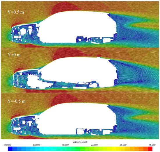
Figure 8.
k−ε Simulation cloud map analysis.
1. Y = 0.5 m. The k-ε model: The velocity distribution may exhibit a uniform decreasing trend (e.g., from 18.00 m/s to 9.00 m/s), indicative of its smoothing capability in high-Reynolds-number flows. In the rear roof region (near the wake zone), the velocity may rapidly decay below 27.00 m/s, suggesting enhanced dissipation of separated flows, which results in blurred vortex structures. K-ω model: A steeper velocity gradient is observed (e.g., a sharp drop from 36.00 m/s to 18.00 m/s), highlighting its sensitivity to curvature variations (e.g., the roof-rear window junction). Velocity fluctuations (e.g., alternating 18.00 m/s and 27.00 m/s) in the wake zone may occur, reflecting a more refined resolution of vortex dissipation dynamics.
2. Y = 0 m. The k-ε model: The underbody region likely displays overall lower velocities (e.g., 0.00–18.00 m/s) due to its reliance on wall functions, which inadequately resolve ground boundary layers and underestimate flow complexity. A velocity peak of 45.00 m/s may prematurely develop near the front bumper, but rapid velocity decay at the rear wheel arch implies a limited separation zone. K-ω model: A stratified velocity distribution is evident, with a stark contrast between the high-speed front region (36.00–45.00 m/s) and low-speed rear region (0.00–9.00 m/s), demonstrating its precise capture of ground effects. Localized low-speed vortex cores (e.g., 9.00 m/s encircling 18.00 m/s) near the rear wheel arch suggest improved prediction of flow separation.
3. Y = −0.5 m. The k-ω model: Velocity in the rear underbody region may significantly decrease to 0.00 m/s, revealing a strong separation zone (e.g., downstream of the diffuser), consistent with experimentally observed separation bubbles. Asymmetric velocity distributions near the front wheels (e.g., 18.00 m/s on the left vs. 27.00 m/s on the right) reflect its adaptability to complex geometries, such as rotating tires.
The simulation results using k-ω turbulence models are analyzed, as shown in Figure 9.
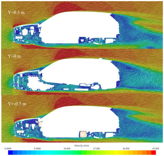
Figure 9.
k-ω simulation cloud map analysis.
The k-e model may be less accurate in capturing the vortices at the rear of the vehicle than the k-o model, resulting in smaller and more dispersed vortices and lower flow velocity. However, the k-o model, due to its suitability for handling near-wall flow, can better capture the formation and shedding of vortices, leading to larger and more concentrated vortices and higher flow velocity.
In industrial practical applications, when rapidly assessing the aerodynamic performance trends of different design schemes, especially in the conceptual design stage where the requirement for calculation accuracy is relatively low, it is more suitable to choose the k-ε model, which has high computational efficiency, requires less computational resources, and can to some extent reflect the overall aerodynamic characteristics trend of the vehicle. In the fine optimization stage, it is necessary to predict the vehicle’s aerodynamic performance more accurately and capture the details of the complex flow field. The DES model has a strong ability to capture the changes in the dynamic flow field under transient operating conditions; the k-ω model performs accurately in predicting key parameters such as lift coefficients and can be used for optimizing specific performance indicators. Therefore, in the fine optimization stage, based on the specific optimization goals, one can flexibly choose the DES model or the k-ω model, or combine their use to obtain more accurate simulation results.
5. Conclusions
This study focuses on the application of virtual wind tunnel simulation technology in vehicle aerodynamic optimization, aiming to improve the prediction accuracy of vehicle aerodynamic performance by combining the authenticity of wind tunnel experiments with the flexibility of computational fluid dynamics (CFD) simulation. Against the backdrop of increasingly severe global energy tension and environmental pollution, optimizing the aerodynamic performance of vehicles is of great significance for reducing fuel consumption and exhaust emissions. The research sets up the computational domains of open field and virtual wind tunnel, precisely sets the boundary conditions, and optimizes the grid strategy, comparing the simulation results of different turbulence models (k-ε, k-ω, and DES) under different operating conditions with wind tunnel experimental data.
The research results indicate that the virtual wind tunnel simulation technology can effectively enhance the prediction accuracy of vehicle aerodynamic performance, providing more effective and accurate technical support for vehicle aerodynamic optimization. Different turbulence models perform differently when dealing with complex flow phenomena. The k-e model performs well in predicting the lag coefficient, with an accuracy of up to 99.22%, while the k-o model is more accurate in predicting the lift coefficient, with an error of only −4.7%; the DES model shows significant advantages under transient operating conditions and allows for more accurate capture of dynamic flow field changes, with an error in drag prediction being as low as 0.3%. Moreover, open-domain simulation is closer to the real free-flow environment, and the simulation results are closer to the test values.
This study provides an important theoretical basis and technical support for the automotive industry to achieve energy saving and emission reduction goals and promote the sustainable development of the automotive industry. By optimizing the aerodynamic performance of vehicles, not only can fuel consumption and exhaust emissions be reduced, but also the driving range of new energy vehicles can be improved, enhancing their market competitiveness. Future research will further explore more efficient turbulent models and simulation technologies to better serve vehicle aerodynamic optimization and the development of the automotive industry.
Author Contributions
Conceptualization, L.W., X.H. and R.M.; Methodology, X.H., P.G., Z.W., J.W., Y.L., Y.Z. and J.D.; Software, L.W., X.H., Z.W., Y.W., J.Z. and X.Y.; Validation, L.W., X.H., P.G. and J.W.; Formal analysis, L.W., X.H., P.G., Z.W., J.W. and Y.M.; Investigation, L.W., P.G., Z.W., J.W., Y.W., Y.M., Y.L. and J.Z.; Resources, X.H., Z.W. and Y.L.; Data curation, X.H., P.G. and Z.W.; Writing—original draft, L.W. and Y.W.; Writing—review & editing, L.W., X.H. and J.W.; Visualization, X.H., P.G., Z.W., J.W., Y.W., Y.M., X.Y., R.M., Y.Z. and J.D.; Supervision, X.H., P.G. and X.Y.; Project administration, X.H., J.W., Y.L., J.Z., X.Y., R.M., Y.Z. and J.D.; Funding acquisition, X.H., J.W., Y.M., Y.L., J.Z., X.Y., R.M., Y.Z. and J.D. All authors have read and agreed to the published version of the manuscript.
Funding
This project was supported by the Jilin Province Science and Technology Development Program, China Grant No. 20220301013GX. Funding amount is 1.2 million RMB.
Data Availability Statement
The datasets presented in this article are not readily available because this project is in the process of being studied and has not yet been fully concluded. Requests to access the datasets should be directed to gp323@jlu.edu.cn.
Conflicts of Interest
Authors Yan Ma, Ying Li, Jing Zhao, Xu Yang, Ruixing Ma, Yinan Zhu and Jianjiao Deng were employed by the company China First Automobile Group Co., Ltd. R & D Institute. The remaining authors declare that the research was conducted in the absence of any commercial or financial relationships that could be construed as a potential conflict of interest.
References
- Katz, J. Automotive Aerodynamics; John Wiley & Sons: Hoboken, NJ, USA, 2016. [Google Scholar]
- Bonnet, J.P. Introduction and fluid mechanics for flow control, Chapter 1. In Fluid Mechanics for Flow Control: Fundamentals, Advances and Applications; Publishing House of Electronics Industry: Beijing, China, 2010. [Google Scholar]
- Bastankhah, M.; Porté-Agel, F. A new miniature wind turbine for wind tunnel experiments. Part I: Design and performance. Energies 2017, 10, 908. [Google Scholar] [CrossRef]
- Siddiqui, N.A.; Agelin-Chaab, M. Investigation of the wake flow around the elliptical ahmed body using detached eddy simulation. Int. J. Heat Fluid Flow 2023, 101, 109125. [Google Scholar] [CrossRef]
- Håkansson, C.; Lenngren, M.J. CFD Analysis of Aerodynamic Trailer Devices for Drag Reduction of Heavy Duty Trucks; Chalmers University of Technology: Göteborg, Sweden, 2010. [Google Scholar]
- Guerrero, A.; Castilla, R.; Eid, G. A Numerical Aerodynamic Analysis on the Effect of Rear Underbody Diffusers on Road Cars. Appl. Sci. 2022, 12, 3763. [Google Scholar] [CrossRef]
- Guo, W.; Liu, X.; Yuan, X. A case study on optimization of building design based on CFD simulation technology of wind environment. Procedia Eng. 2015, 121, 225–231. [Google Scholar] [CrossRef]
- Cravero, C.; Marsano, D. Computational Investigation of the Aerodynamics of a Wheel Installed on a Race Car with a Multi-Element Front Wing. Fluids 2022, 7, 182. [Google Scholar] [CrossRef]
- Fernandez-Gamiz, U.; Gomez-Mármol, M.; Chacón-Rebollo, T. Computational Modeling of Gurney Flaps and Microtabs by POD Method. Energies 2018, 11, 2091. [Google Scholar] [CrossRef]
- Li, T.; Dai, Z.; Liu, J.; Wu, N.; Zhang, W. Review on aerodynamic drag reduction optimization of high-speed trains in China. J. Traffic Transp. Eng. 2021, 21, 59–80. [Google Scholar]
- Liao, G.; Xue, M.; Yue, L.; Yang, H.; Guo, P.; Hu, X.; Wang, Z.; Ma, T. Passive Drag Reduction Optimization for Complex Commercial Vehicle Models. J. Appl. Fluid Mech. 2025, 18, 1639–1651. [Google Scholar]
- Shao, J.; Zuo, H.; Hu, X. Aerodynamic drag reduction optimization of an SUV and its flow field mechanism. Automot. Eng. 2024, 46, 356–365. [Google Scholar] [CrossRef]
- Gollamudi, S.; Kamali, H.; Fauchoux, M.; Krishnan, E.; Joseph, A.; Simonson, C. Coupled ϵ-NTU to design and evaluate the performance of energy exchangers with coupled heat and mass transfer. ASME J. Heat Mass Transf. 2025, 147, 081901. [Google Scholar] [CrossRef]
- Bandi, P.; Manelil, N.P.; Maiya, M.P.; Tiwari, S.; Thangamani, A.; Tamalapakula, J.L. Influence of flow and thermal characteristics on thermal comfort inside an automobile cabin under the effect of solar radiation. Appl. Therm. Eng. 2022, 203, 117946. [Google Scholar] [CrossRef]
- Spalart, P.R. Detached-Eddy Simulation. Annu. Rev. Fluid Mech. 2009, 41, 181–202. [Google Scholar]
- Ferziger, J.H.; Perić, M. Computational Methods for Fluid Dynamics; Springer: Berlin/Heidelberg, Germany, 2002. [Google Scholar]
- Cinosi, N.; Walker, S.P.; Bluck, M.J.; Issa, R. CFD simulation of turbulent flow in a rod bundle with spacer grids (MATIS-H) using STAR-CCM+. J. Nucl. Eng. Des. 2014, 279, 37–49. [Google Scholar] [CrossRef]
- Menter, F.R. Two-equation eddy-viscosity turbulence models for engineering applications. AIAA J. 1994, 32, 1598–1605. [Google Scholar] [CrossRef]
- Huang, T.; Liu, J.; He, X.; Bu, H.; Wang, Q.; Xu, S.; Zhu, X. Extended study of full-scale wind tunnel test and simulation analysis based on DrivAer model. Proc. Inst. Mech. Eng. Part D J. Automob. Eng. 2022, 236, 2433–2447. [Google Scholar] [CrossRef]
Disclaimer/Publisher’s Note: The statements, opinions and data contained in all publications are solely those of the individual author(s) and contributor(s) and not of MDPI and/or the editor(s). MDPI and/or the editor(s) disclaim responsibility for any injury to people or property resulting from any ideas, methods, instructions or products referred to in the content. |
© 2025 by the authors. Licensee MDPI, Basel, Switzerland. This article is an open access article distributed under the terms and conditions of the Creative Commons Attribution (CC BY) license (https://creativecommons.org/licenses/by/4.0/).