
Research on Energy Regeneration Characteristics of Multi-Link Energy-Fed Suspension


Abstract
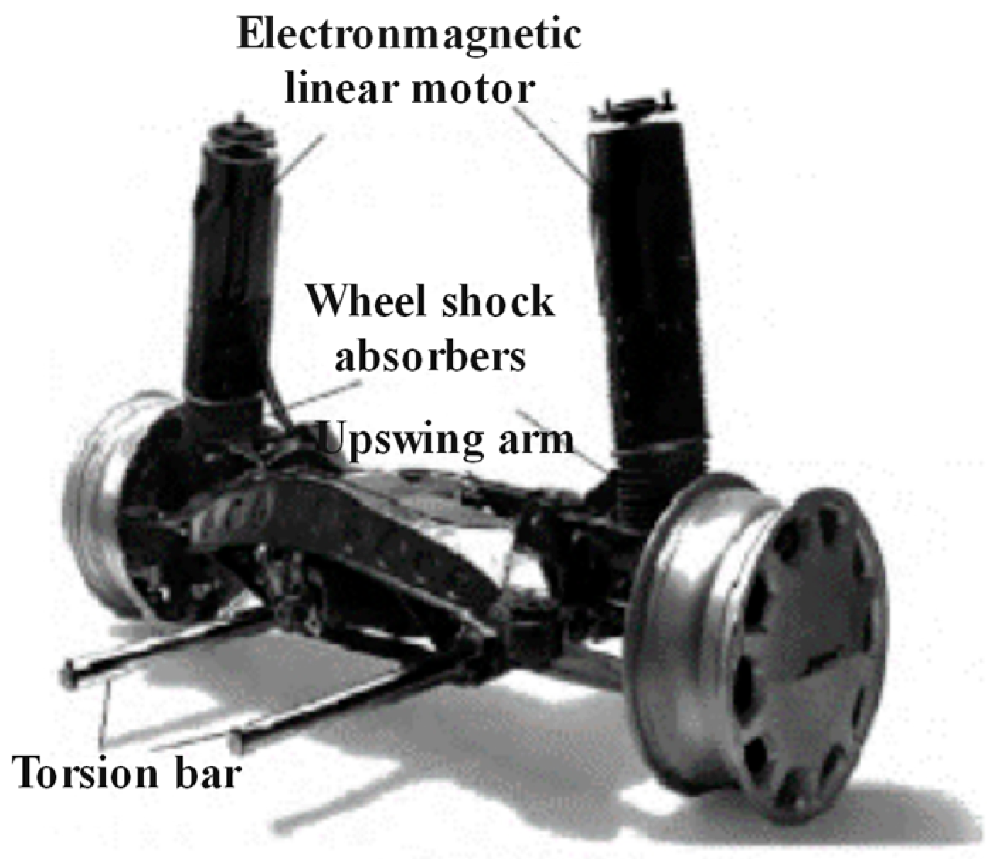
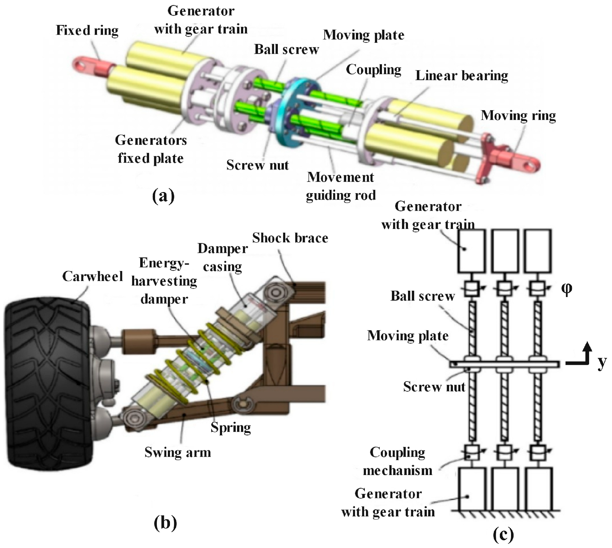
1. Introduction
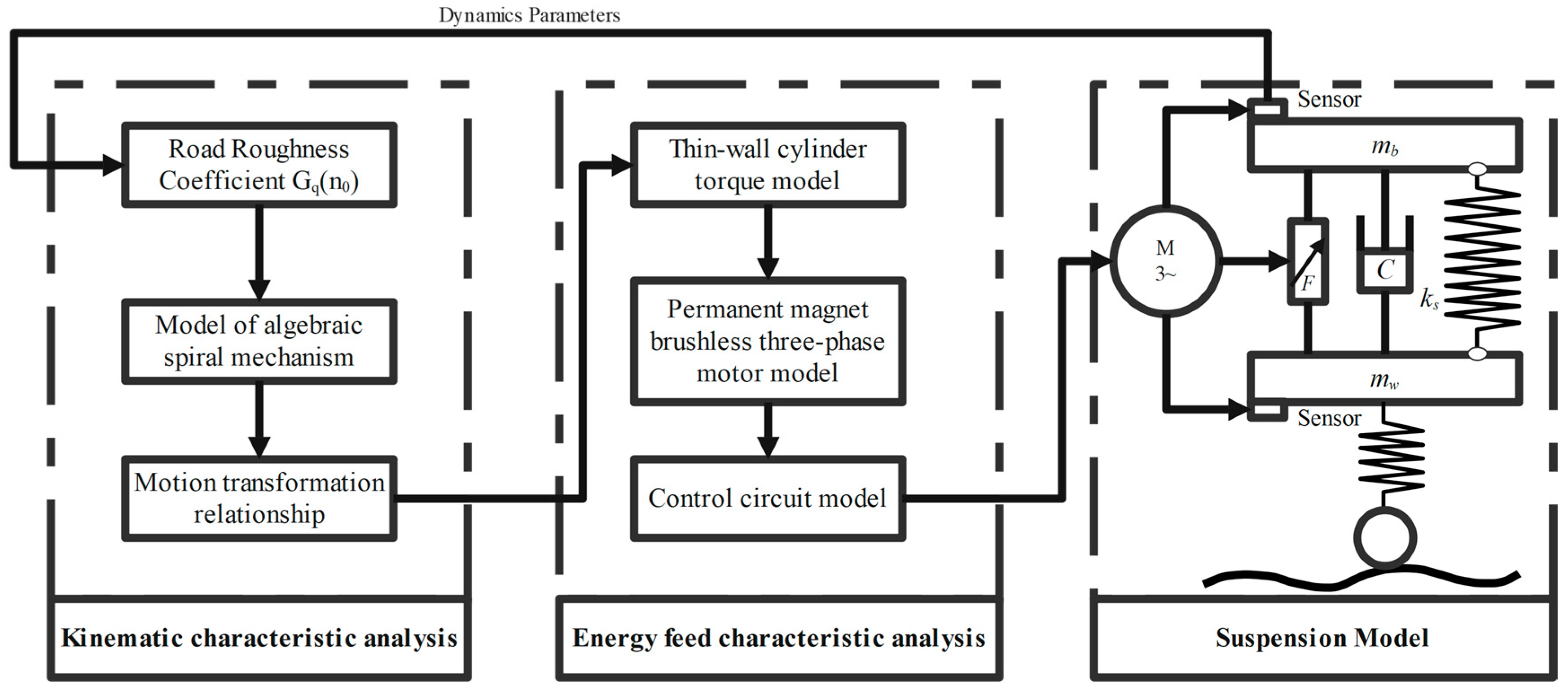
2. System Modeling
2.1. Two-Degree-of-Freedom 1/4 Vehicle Modeling
- (1)
- The interior and various parts of the vehicle are rigid bodies, without deformation;
- (2)
- The vehicle’s mass is uniformly distributed between the two centers of mass, located in the body and the chassis;
- (3)
- The vehicle only moves in the vertical direction, without considering the movement of the vehicle in the horizontal direction;
- (4)
- The suspension system is a linear elastic element, without considering nonlinear effects;
- (5)
- The wheels remain vertical in the vertical direction, ignoring the rolling and pitching of the wheels;
- (6)
- The vehicle maintains the same speed when turning, without considering the change in the acceleration of the vehicle in actual driving.
2.2. Modeling of Random Pavement Input
3. Analysis of Motion Characteristics
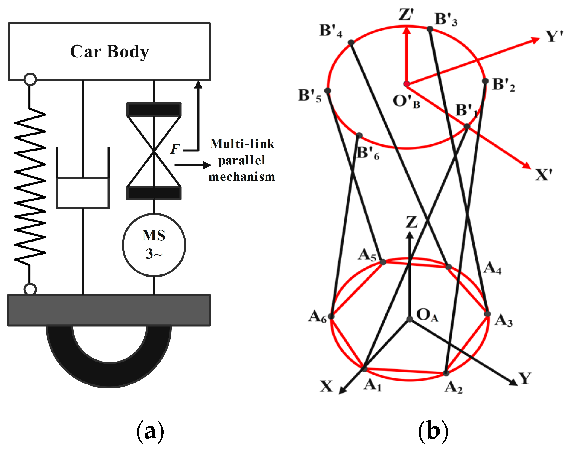
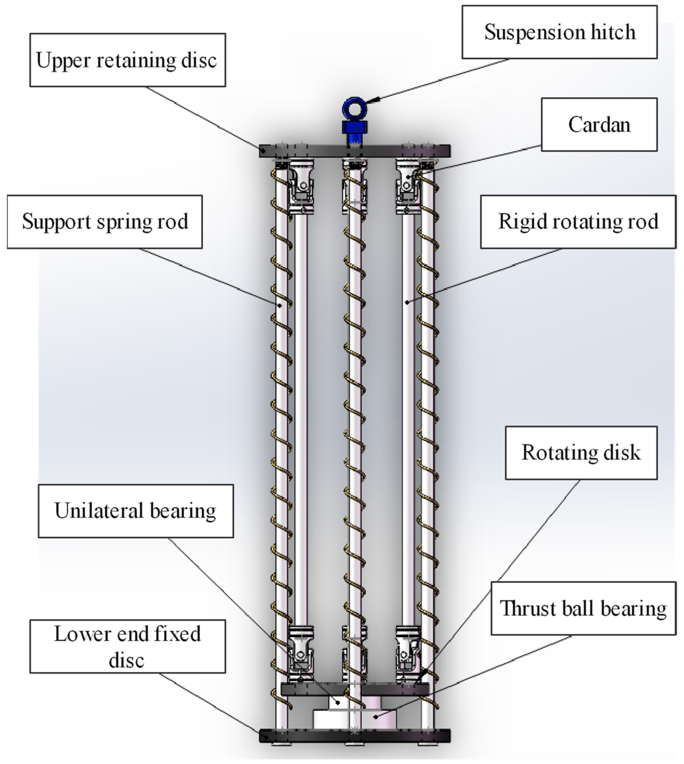
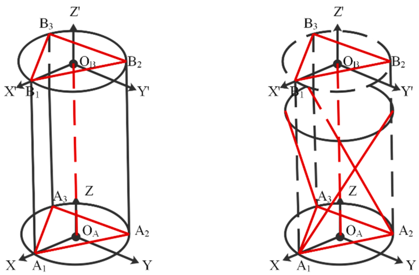
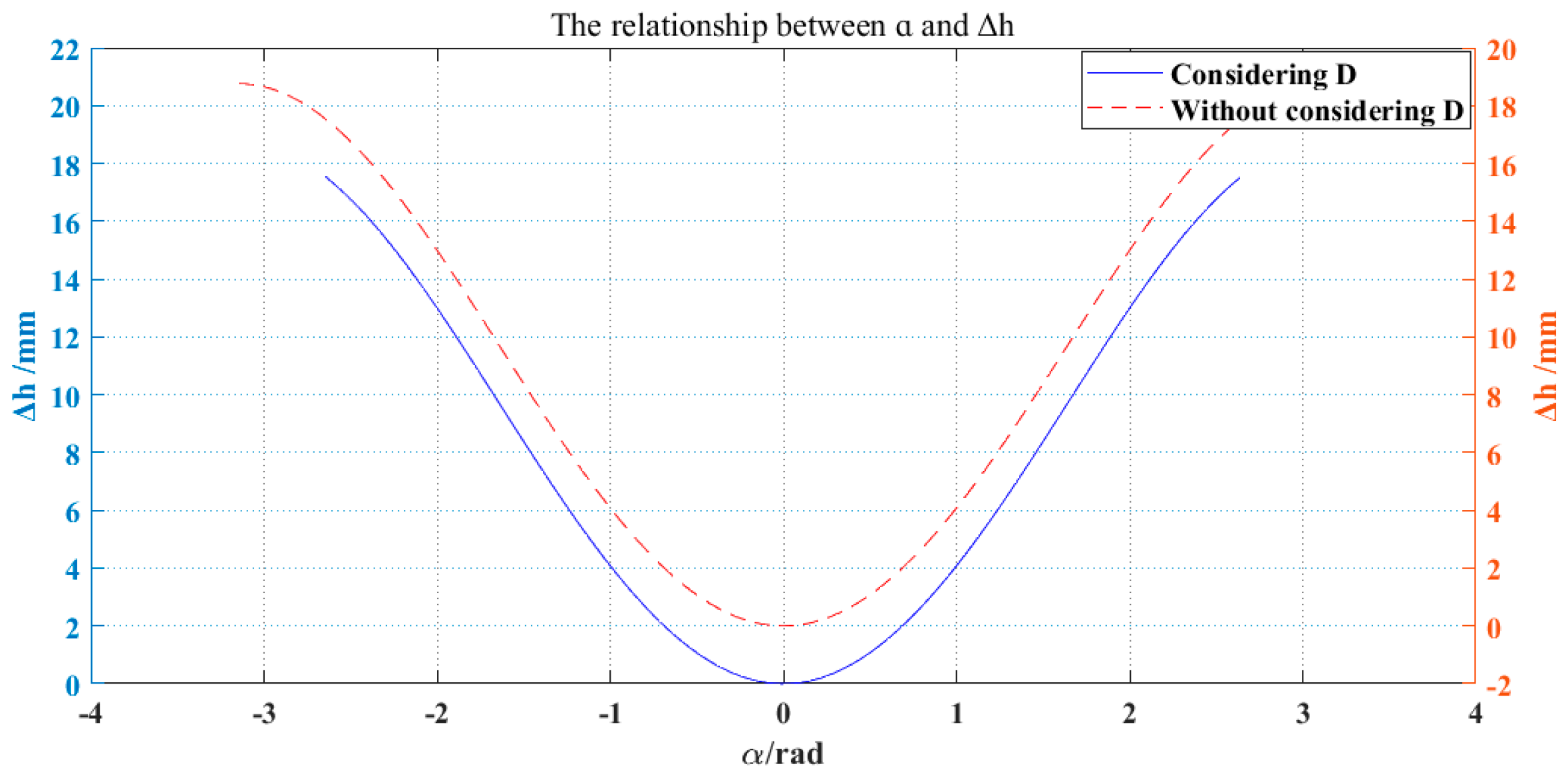
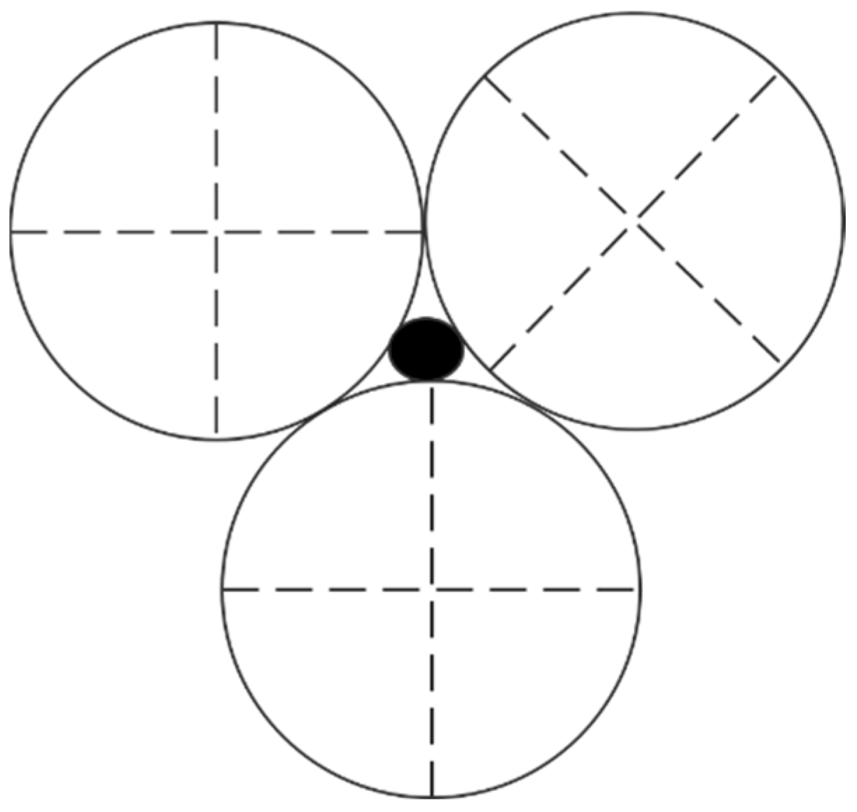
3.1. Multi-Link Parallel Mechanism
3.2. Modeling of Algebraic Helical Mechanisms
3.3. Simulation of Motion Transformation Relationship
4. Analysis of Energy Feed Characteristics
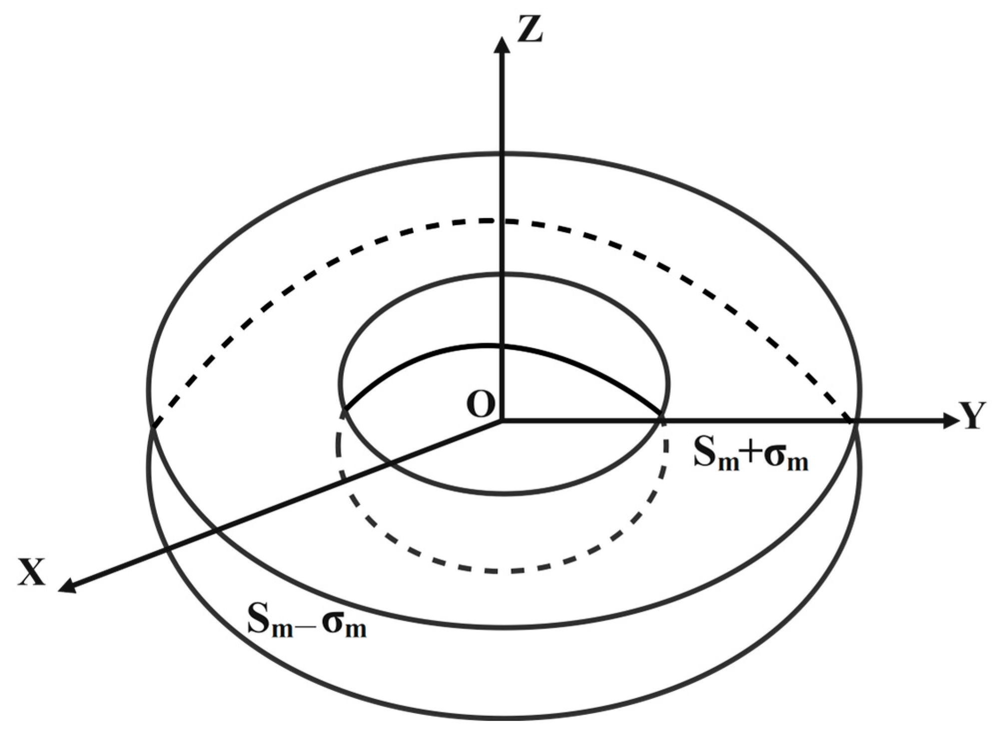
4.1. Torsion Model of Imaginary Thin-Walled Cylinder
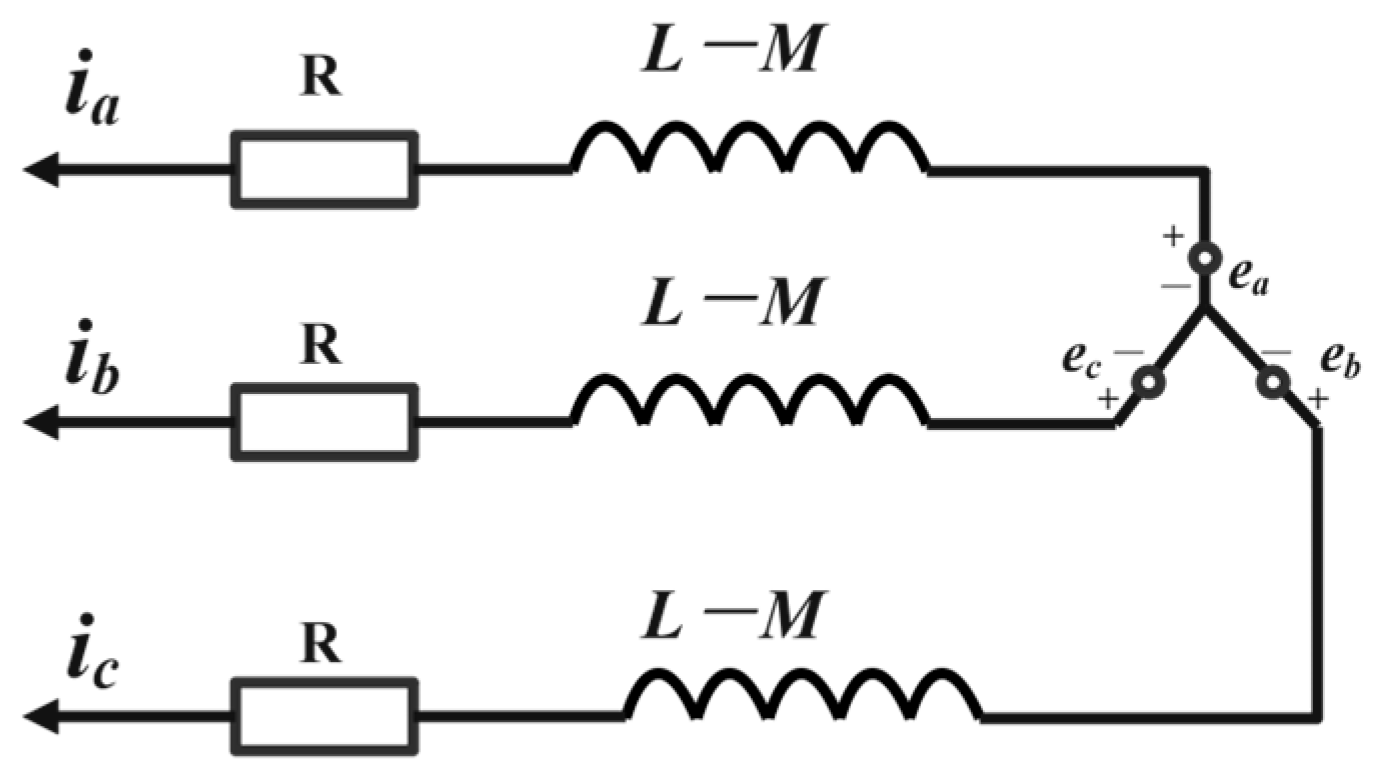
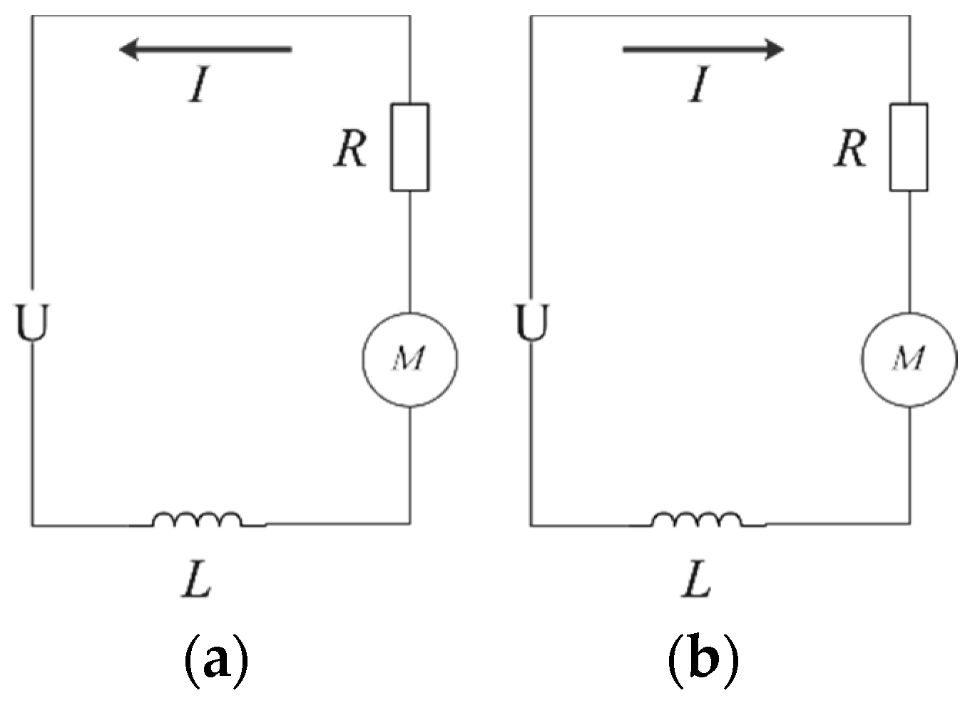
4.2. Modeling of Permanent Magnet Brushless Three-Phase Motor
- (1)
- The electrical conductivity of permanent magnet material is zero;
- (2)
- The armature winding is distributed on the inner side of the stator;
- (3)
- There is no saturation in the magnetic circuit of the motor;
- (4)
- The armature magnetic motive force generated when the motor winding through the current is not considered;
- (5)
- The parameters of the motor are not changed by temperature fluctuations;
- (6)
- The motor parameters do not change with frequency changes;
- (7)
- The stator current and rotor magnetic field are arranged in square wave symmetry in the motor;
- (8)
- The three-phase stator is wound to form a center symmetrical arrangement.
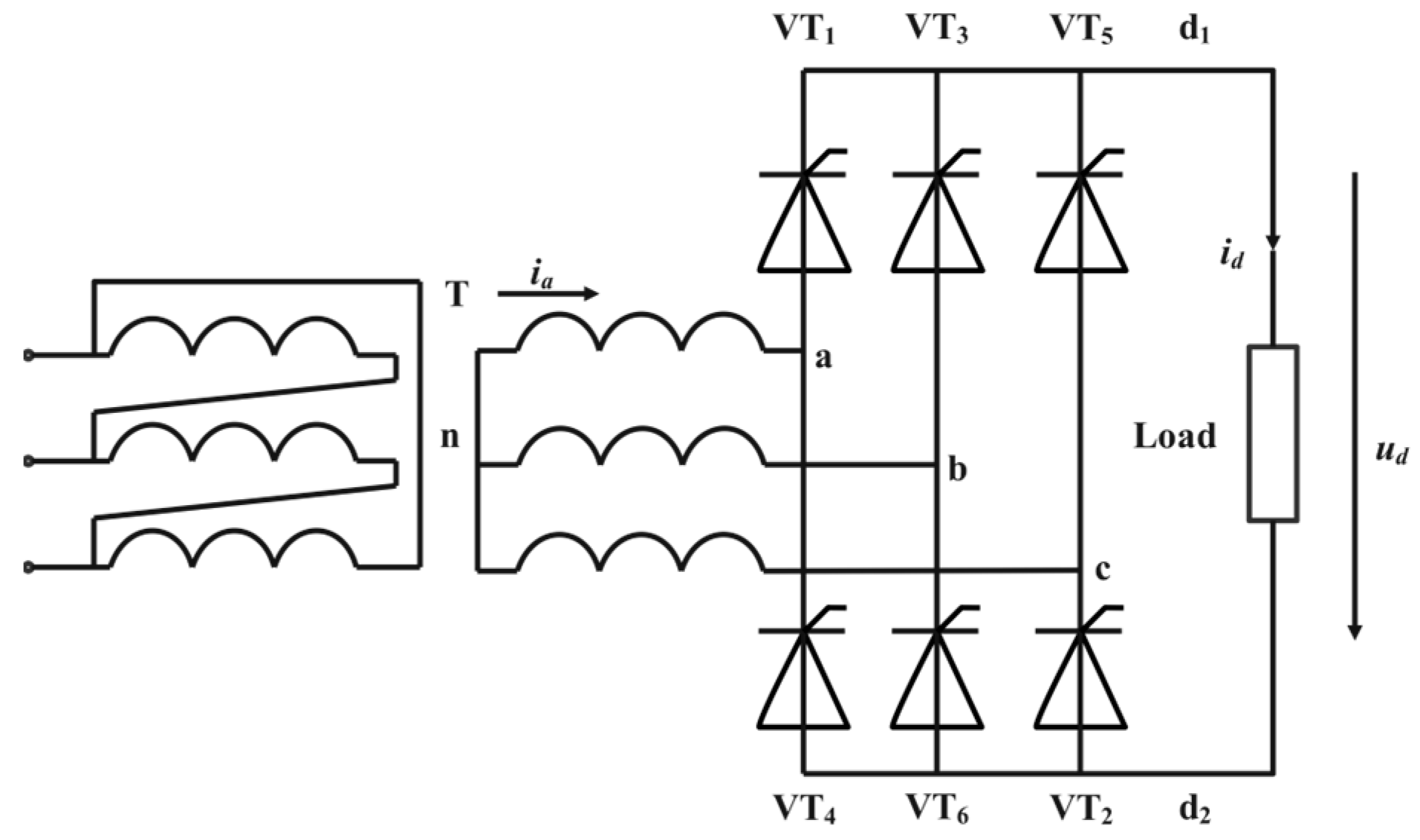
4.3. Modeling of Control Circuit
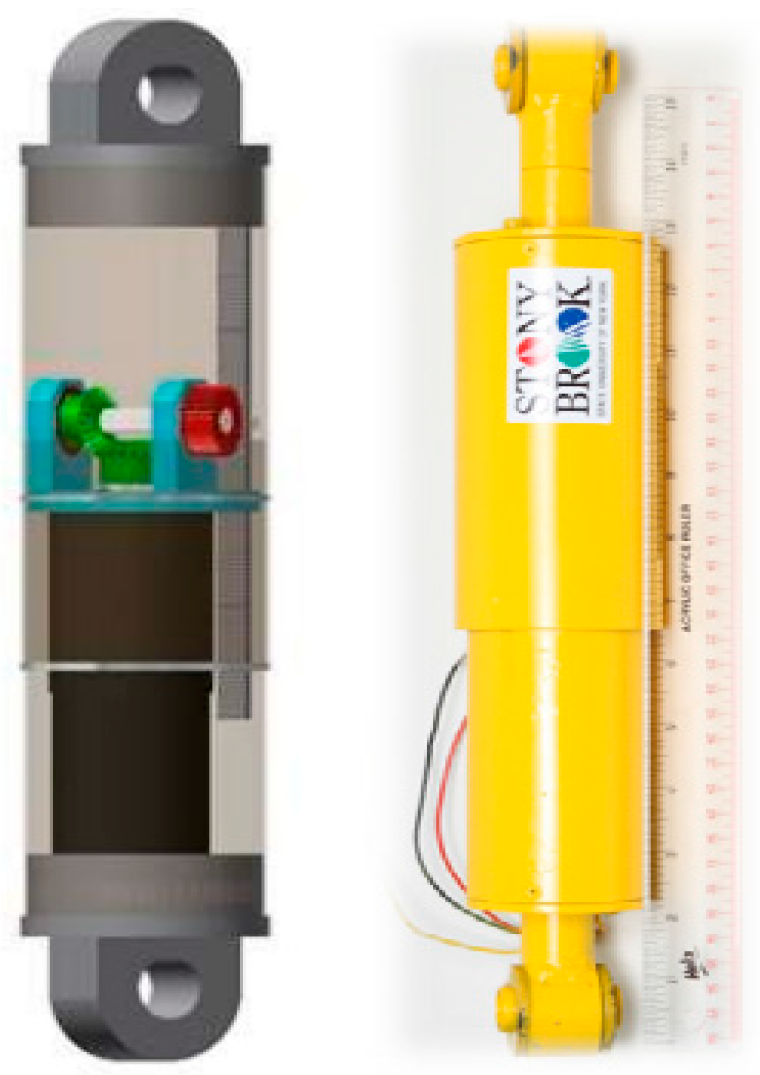
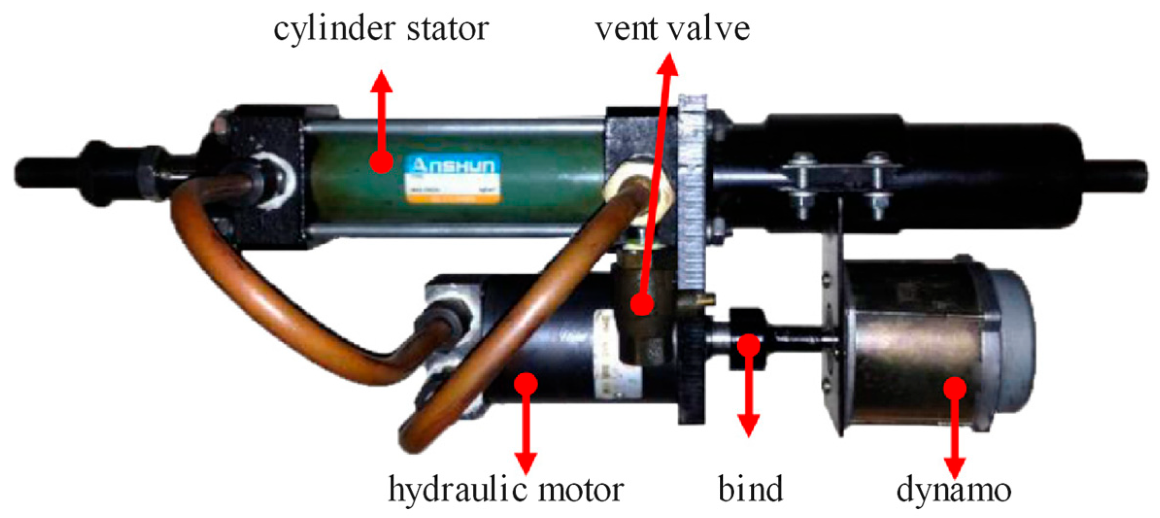
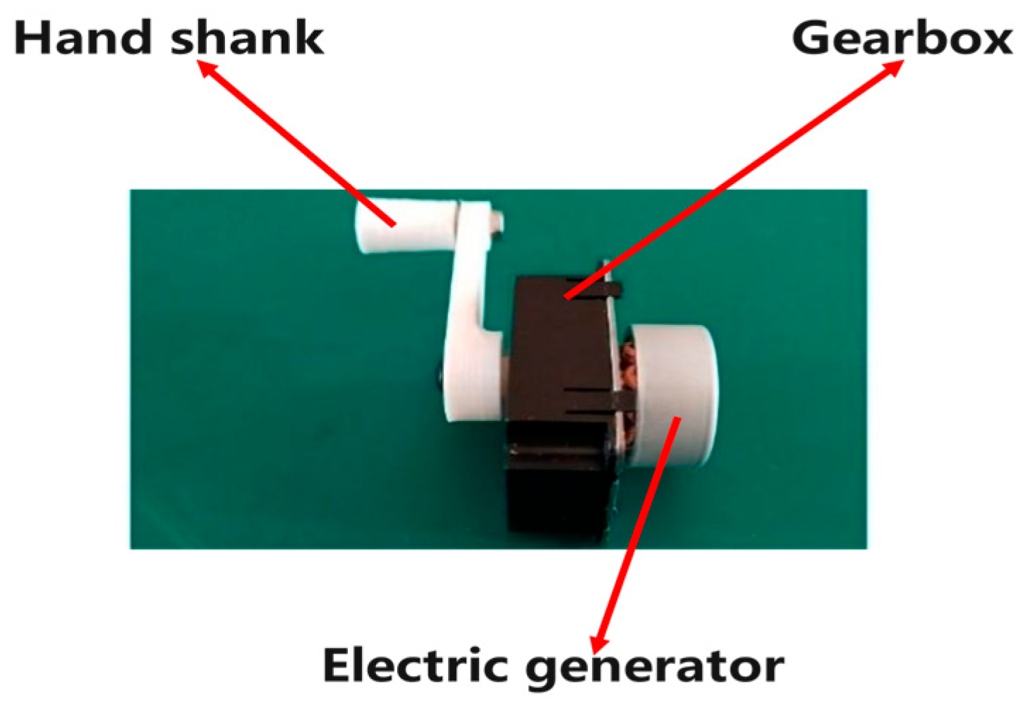
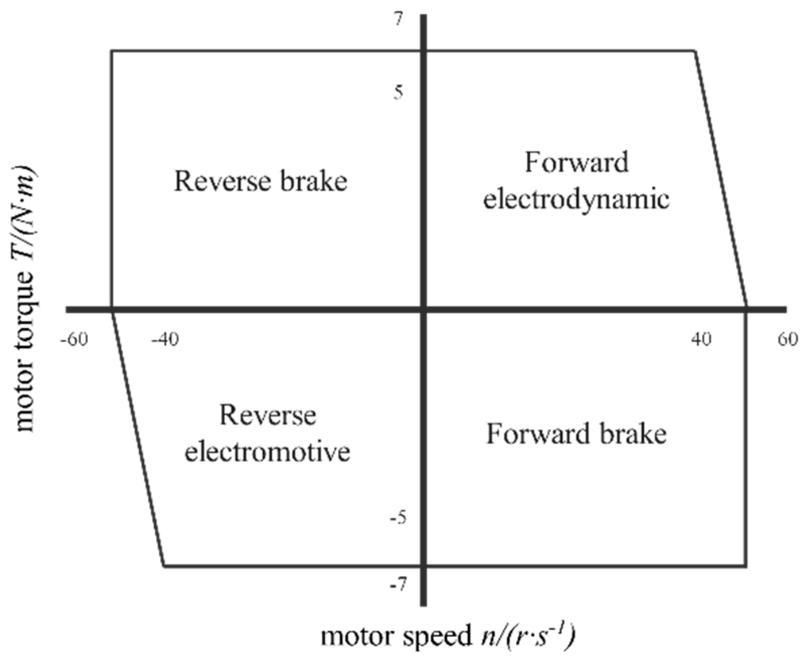
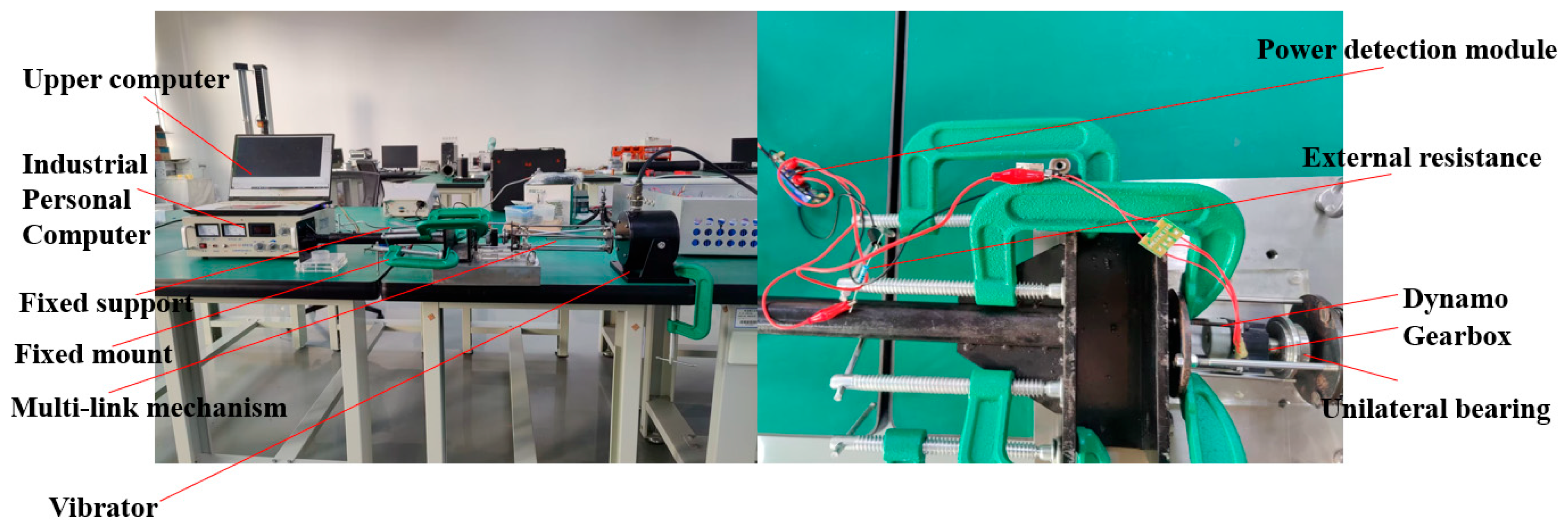
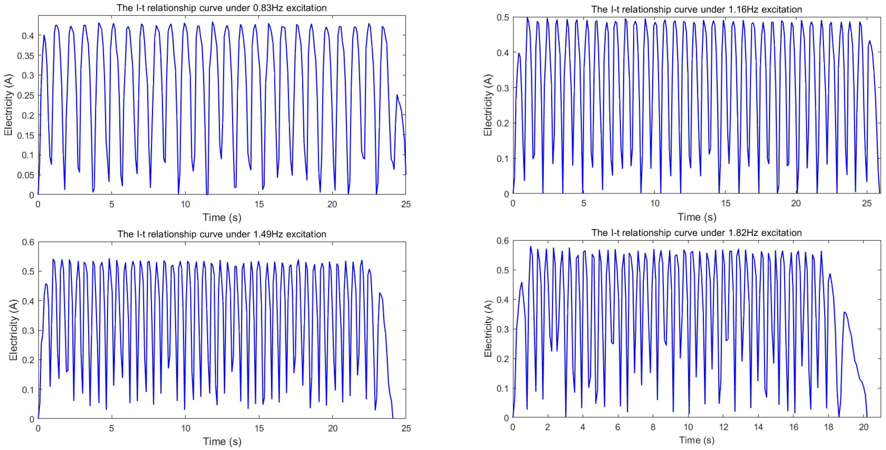
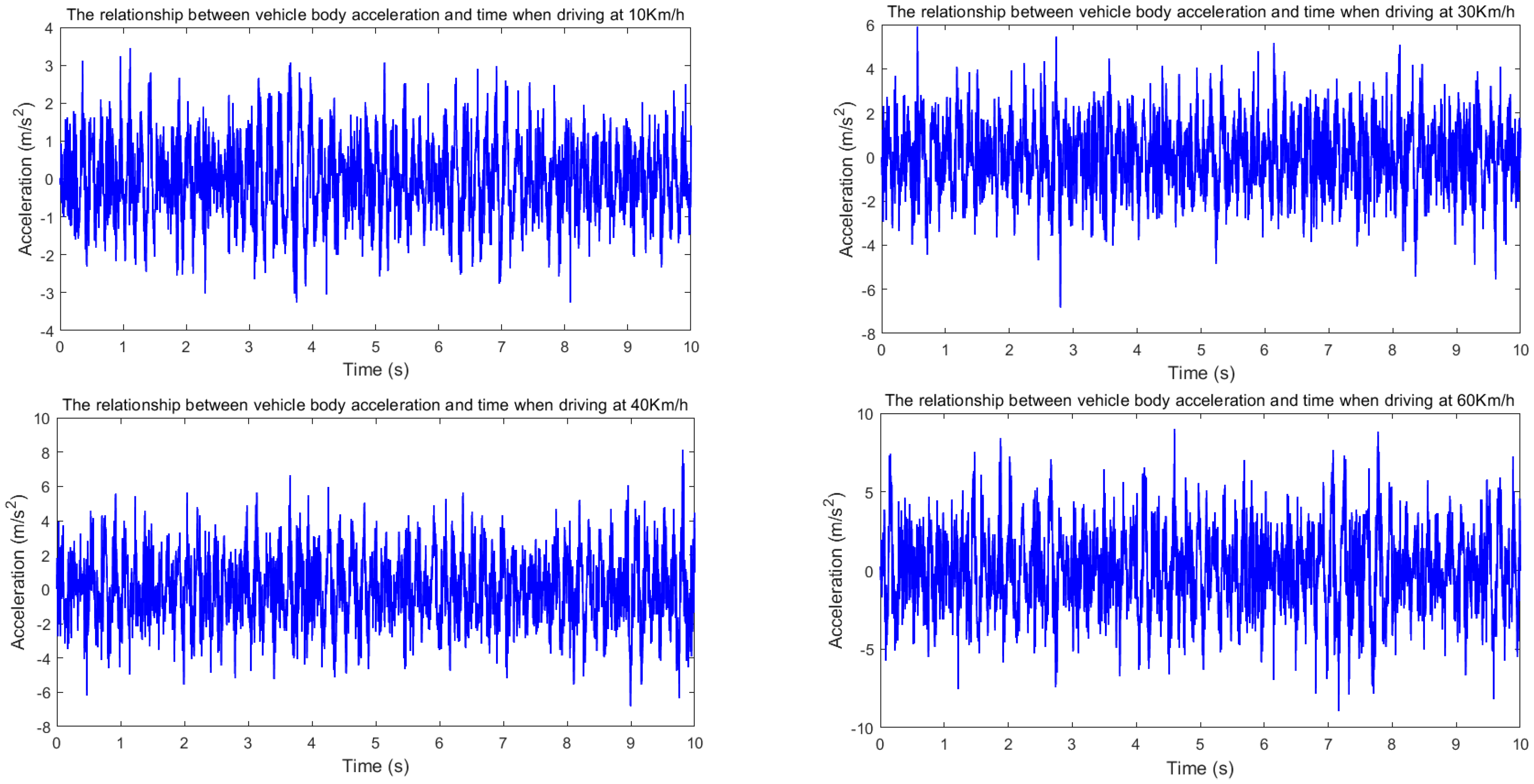
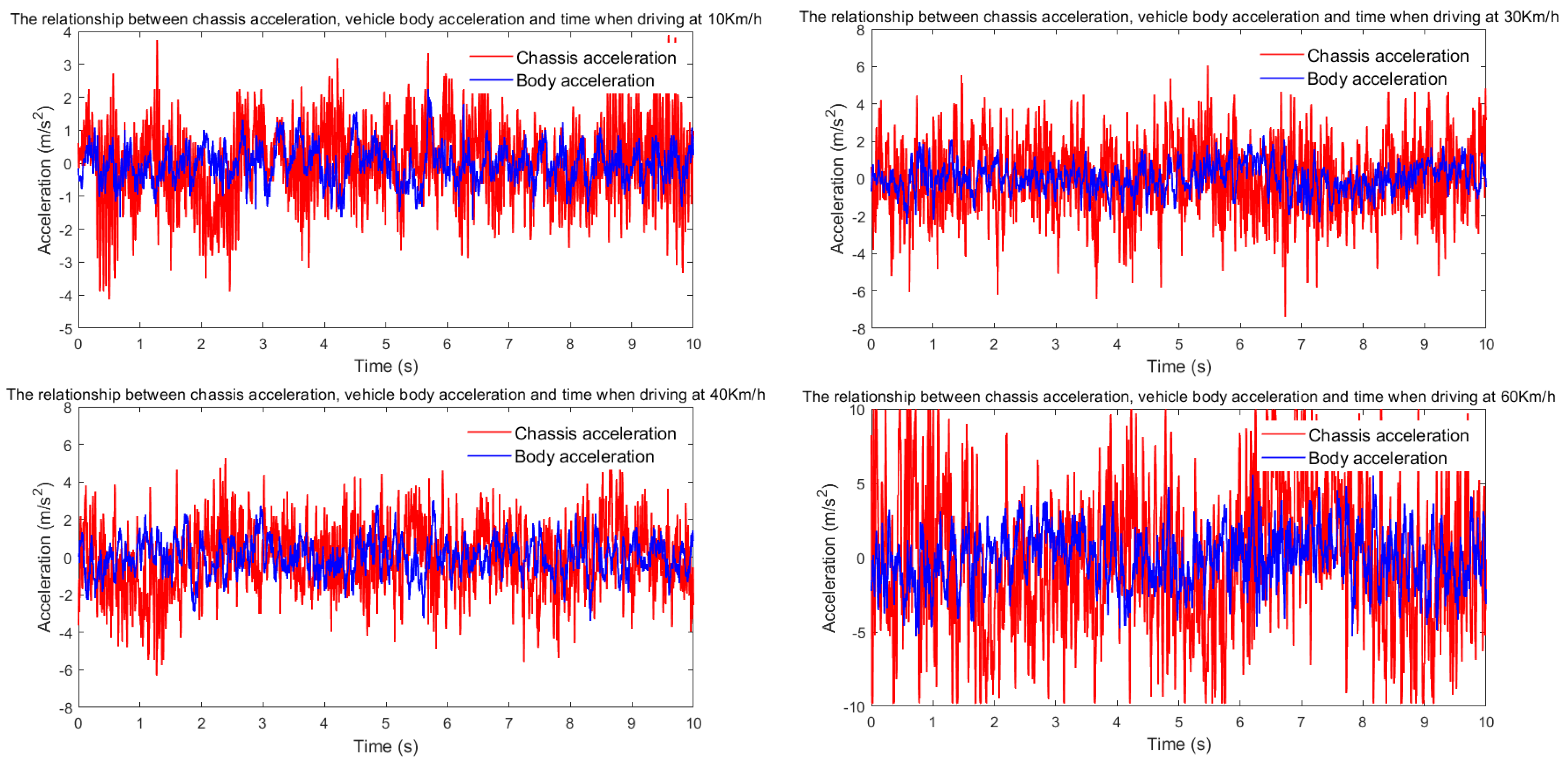
5. Prototype Test and Analysis
6. Conclusions
Author Contributions
Funding
Data Availability Statement
Conflicts of Interest
References
- Wang, S.; Lv, Y.; Zhang, S.; Liu, Z. Research Progress on Control Strategy of Automotive Active Suspension System. Automot. Parts 2016, 5, 82–85. [Google Scholar]
- Abdelkareem, M.A.A.; Eldaly, A.B.M.; Ali, M.K.A.; Youssef, I.M.; Xu, L. Monte Carlo sensitivity analysis of vehicle suspension energy harvesting in frequency domain. J. Adv. Res. 2020, 24, 53–67. [Google Scholar] [CrossRef] [PubMed]
- Luo, R.; Yu, Z.; Wu, P.; Hou, Z. Analytical solutions of the energy harvesting potential from vehicle vertical vibration based on statistical energy conservation. Energy 2023, 264, 126111. [Google Scholar] [CrossRef]
- Liu, J.; Liu, J.; Zhang, X.; Liu, B. Transmission and energy-harvesting study for a novel active suspension with simplified 2-DOF multi-link mechanism. Mech. Mach. Theory 2021, 160, 104286. [Google Scholar] [CrossRef]
- Zhang, R.; Zhao, L.; Qiu, X.; Zhang, H.; Wang, X. A comprehensive comparison of the vehicle vibration energy harvesting abilities of the regenerative shock absorbers predicted by the quarter, half and full vehicle suspension system models. Appl. Energy 2020, 272, 115180. [Google Scholar] [CrossRef]
- Chen, L.; Zhou, K.; Li, Z. Dynamic Characteristic Fitting of Air Spring and Calculation and Analysis of Variable Stiffness of Air Suspension. Chin. J. Mech. Eng. 2010, 46, 93–98. [Google Scholar] [CrossRef]
- Guo, Y.; Wang, B.; Tkachev, A.; Zhang, N. An LQG Controller Based on Real System Identification for an Active Hydraulically Interconnected Suspension. Math. Probl. Eng. 2020, 1, 6669283. [Google Scholar] [CrossRef]
- Dai, J.; Wang, C.; Liu, Z.; Zhu, J.; Hu, X. Research review of Energy-fed suspension technology. Sci. Technol. Eng. 2018, 30, 131–139. [Google Scholar]
- Chen, S.; Sun, W.; Wang, J.; Zhao, L.; Cai, Y. Control of linear motor energy-fed semi-active suspension based on variable voltage charging method. J. Traffic Transp. Eng. 2018, 18, 90–100. [Google Scholar]
- Pei, J.; Li, Y.; Wang, Y.; Sun, W.; Zheng, L. Design and Energy Analysis of Active Suspension Control System Using Electromagnetic Linear Motor. Automot. Eng. 2014, 36, 1386–1391. [Google Scholar]
- Gupta, A.; Jendrzejczyk, J.A.; Mulcahy, T.M.; Hull, J.R. Design of electromagnetic shock absorbers. Int. J. Mech. Mater. Des. 2006, 3, 285–291. [Google Scholar] [CrossRef]
- Xie, L.; Li, J.; Li, X.; Huang, L.; Cai, S. Damping-tunable energy-harvesting vehicle damper with multiplecontrolled generators: Design, modeling and experiments. Mech. Syst. Signal Process. 2018, 99, 859–872. [Google Scholar] [CrossRef]
- Song, X.; Li, Z.; Edmondson, J.R. Regenerative passive and semi-active suspension. U.S. Patent 7,087,342, 8 August 2006. [Google Scholar]
- Li, Z.; Zuo, L.; Luhrs, G.; Lin, L.; Qin, Y.X. Electromagnetic energy-harvesting shock absorbers: Design, modeling, and road tests. IEEE Trans. Veh. Technol. 2012, 62, 1065–1074. [Google Scholar] [CrossRef]
- Mi, J.; Xu, L.; Guo, S.; Meng, L.; Abdelkareem, M.A. Energy harvesting potential comparison study of a novel railwayvehicle bogie system with the hydraulic-electromagnetic energy-regenerative shock absorber. In Proceedings of the ASME/IEEE Joint Rail Conference, Philadelphia, PA, USA, 19 July 2017; American Society of Mechanical Engineers: New York, NY, USA, 2017; Volume 50718, p. V001T07A004. [Google Scholar]
- Fang, Z.; Guo, X.; Xu, L.; Zhang, H. An optimal algorithm for energy recovery of hydraulic electromagnetic energy-regenerative shock absorber. Appl. Math. Inf. Sci. 2013, 7, 2207. [Google Scholar] [CrossRef]
- Li, C.; Zhu, R.; Liang, M.; Yang, S. Integration of shock absorption and energy harvesting using a hydraulic rectifier. J. Sound Vib. 2014, 333, 3904–3916. [Google Scholar] [CrossRef]
- Li, P.; Zuo, L.; Lu, J.; Xu, L. Electromagnetic regenerative suspension system for ground vehicles. In Proceedings of the 2014 IEEE International Conference on Systems, Man, and Cybernetics (SMC), San Diego, CA, USA, 5–8 October 2014; IEEE: Piscataway, NJ, USA, 2014; pp. 2513–2518. [Google Scholar]
- Abdelkareem, M.A.A.; Xu, L.; Guo, X.; Ali, M.K.A.; Elagouz, A.; Hassan, M.A.; Essa, F.A.; Zou, J. Energy harvesting sensitivity analysis and assessment of the potential power and full car dynamics for different road modes. Mech. Syst. Signal Process. 2018, 110, 307–332. [Google Scholar] [CrossRef]
- Hajidavalloo, M.R.; Cosner, J.; Li, Z.; Tai, W.C.; Song, Z. Simultaneous suspension control and energy harvesting through novel design and control of a new nonlinear energy harvesting shock absorber. IEEE Trans. Veh. Technol. 2022, 71, 6073–6087. [Google Scholar] [CrossRef]
- Geng, Z.J.; Haynes, L.S. Six degree-of-freedom active vibration controlusingthe Stewart platforms. IEEE Trans. Control. Syst. Technol. 1994, 2, 45–53. [Google Scholar] [CrossRef]
- Wang, Z.; Zhou, Z.; Ruan, L.; Duan, X.; Wang, Q. Mechatronic design and control of a rigid-soft hybrid knee exoskeleton for gait intervention. IEEE/ASME Trans. Mechatron. 2023, 28, 2553–2564. [Google Scholar] [CrossRef]


| Grade of Pavement | Lower Limit | Geometric Mean | Upper Limit |
|---|---|---|---|
| A | 8 | 16 | 32 |
| B | 32 | 64 | 128 |
| C | 128 | 256 | 512 |
| D | 512 | 1024 | 2048 |
| E | 2048 | 4096 | 8192 |
| F | 8192 | 16,384 | 32,768 |
| G | 32,768 | 65,536 | 131,072 |
| H | 131,072 | 262,144 | 524,288 |
| Excitation Frequency (Hz) | Maximum Excitation Current (A) | Maximum Excitation Current Per Second (A) | Maximum Excitation Power (W) | Maximum Excitation Voltage (V) | Drive Motor Speed (r/min) | Resistance (Ω) |
|---|---|---|---|---|---|---|
| 0.83 | 0.43 | 0.0172 | 9.39 | 21.66 | 50 | 50 |
| 1.16 | 0.50 | 0.0192 | 12.44 | 24.94 | 70 | 50 |
| 1.49 | 0.54 | 0.0216 | 14.73 | 27.14 | 90 | 50 |
| 1.82 | 0.58 | 0.0276 | 16.84 | 29.01 | 110 | 50 |
| Performance Indicator (Unit) | RMS | Inhibition Ratio | |
|---|---|---|---|
| BA (m/s2)-10 km/h | 0.9789 | 0.5441 | 44.42% |
| BA (m/s2)-30 km/h | 1.5970 | 0.8311 | 47.96% |
| BA (m/s2)-40 km/h | 2.0134 | 0.9690 | 51.87% |
| BA (m/s2)-60 km/h | 2.4834 | 1.8628 | 24.99% |
Disclaimer/Publisher’s Note: The statements, opinions and data contained in all publications are solely those of the individual author(s) and contributor(s) and not of MDPI and/or the editor(s). MDPI and/or the editor(s) disclaim responsibility for any injury to people or property resulting from any ideas, methods, instructions or products referred to in the content. |
© 2025 by the authors. Licensee MDPI, Basel, Switzerland. This article is an open access article distributed under the terms and conditions of the Creative Commons Attribution (CC BY) license (https://creativecommons.org/licenses/by/4.0/).
Share and Cite
Zhang, X.; Liu, J.; Li, Y.; Wang, G.; Zou, Y.; Liu, J. Research on Energy Regeneration Characteristics of Multi-Link Energy-Fed Suspension. Energies 2025, 18, 2743. https://doi.org/10.3390/en18112743
Zhang X, Liu J, Li Y, Wang G, Zou Y, Liu J. Research on Energy Regeneration Characteristics of Multi-Link Energy-Fed Suspension. Energies. 2025; 18(11):2743. https://doi.org/10.3390/en18112743
Chicago/Turabian StyleZhang, Xuefeng, Jianze Liu, Yang Li, Guangzheng Wang, Yu Zou, and Jiang Liu. 2025. "Research on Energy Regeneration Characteristics of Multi-Link Energy-Fed Suspension" Energies 18, no. 11: 2743. https://doi.org/10.3390/en18112743
APA StyleZhang, X., Liu, J., Li, Y., Wang, G., Zou, Y., & Liu, J. (2025). Research on Energy Regeneration Characteristics of Multi-Link Energy-Fed Suspension. Energies, 18(11), 2743. https://doi.org/10.3390/en18112743