1. Introduction
Natural disasters (such as earthquakes, hurricanes, and floods), human-made disasters (such as terrorist attacks and cyber attacks), and equipment aging can lead to power system failures, resulting in widespread power outages. Between 2017 and 2020, approximately 100 million people were affected by extreme weather each year [
1]. In the United States, weather-related power outages caused up to USD 55 billion losses annually [
2]. This reflects the importance of ensuring the resilience of the power system in the face of extreme events.
In traditional load restoration methods, scholars have made significant progress. Early research focused on the design of black-start schemes, gradually restoring network architecture through the self-starting capability of thermal power units or microgrid systems [
3,
4]. With the increasing penetration rate of renewable energy, research gradually shifted towards multi-timescale collaborative optimization [
5,
6]. However, traditional methods still have limitations in dealing with load dynamics, source–load interactions, and communication dependencies.
Integrating flexible resources is another effective method to help with rapid load restoration [
7,
8]. At present, there are two main flexible resource coordination mechanisms for power supply reconstruction: the first is the complementary scheduling of traditional power generation units and distributed power sources [
9]; the second is the dynamic configuration of mobile energy storage devices, emergency power generation equipment, and multigrid coupling devices based on energy coupling characteristics [
10]. However, the above research only considered achieving rapid load restoration by scheduling flexible resources on the power supply side, and did not fully consider the impact of the demand side on the restoration method.
In extreme disasters, the speed and efficiency of load recovery are crucial. Although the traditional black-start scheme and multi-timescale collaborative optimization method are effective, they also have some limitations. First, black-start scheme depends on the self-starting ability of thermal power units or microgrid systems, which may take a long time to restore power supply, and in some cases, the starting process of thermal power units may be limited by fuel supply and equipment status. Secondly, although multi-timescale collaborative optimization can improve the overall efficiency of the system, its complexity and dependence on real-time data may lead to delays in response time.
In contrast, demand response, as a flexible load management strategy, can accelerate the restoration process of the power grid by encouraging users to reduce power consumption during peak demand periods or rapidly increase their load after power supply restoration. DR has two advantages: First, it reduces the complexity of the recovery path. While traditional black-start schemes need to restore the line and power level by level, DR reduces the dependence on line operation time by dynamically adjusting the demand-side loads. Second, it enhances the robustness of the system. Traditional methods are vulnerable to power node failures. However, DR can maintain power supply in key areas through flexible adjustment on the demand side to improve recovery reliability by taking advantage of the dispersion of resources on the load side, even if part of the power supply fails. In addition, demand response can flexibly respond to the actual demand changes in the power grid through real-time feedback and dynamic adjustment, avoiding the problems of resource waste and inefficiency that may occur in traditional methods. Therefore, demand response can not only effectively supplement the shortcomings of traditional methods, but also improve the resilience and flexibility of the overall power grid, providing a new solution for load recovery after extreme disasters.
Under extreme disasters, user-side resources have faster response speeds and more flexible regulation capabilities [
11], which can effectively enhance the system’s resilience and promote load restoration [
12,
13]. Therefore, this article considers DR as a flexible resource and explores its positive role in load restoration. At present, there have been numerous studies on the application of DR in load restoration scenarios in the existing literature. Reference [
14] constructed a coupon incentive model to optimize the social profits of DR. Reference [
15] accelerated post-disaster load restoration by integrating mobile emergency generators with producer and consumer communities and coordinating supply- and demand-side resources. Reference [
16] established an operational optimization model for residential DR and distribution network restoration, utilizing DR to assist in the rapid restoration of the distribution network. Reference [
17] proposed a price-based DR method for aggregate temperature-controlled loads for load frequency control. Reference [
18] proposed a direct load control (DLC) and load shedding method to minimize power outages and reduce the peak-to-average load ratio in the event of sudden changes in grid load. The above literature demonstrates the potential of incentive-based response in terms of price and purchasing method. However, it ignores users’ proactive response behavior (such as economic profits, comfort preferences, etc.), which affects the practicality of the method. In practical situations, most consumers may not be interested in DR strategies or lack motivation to participate, especially without incentives.
This article proposes a bi-level optimization method for load restoration under extreme events based on a symmetrical DR incentive mechanism. This method coordinates the profit of the grid and user sides by constructing a bi-level optimization model. The upper-level model aims to minimize the cost of load restoration on the grid side and optimize decision variables including the user energy supply ratio, incentive coefficients, and response clearing quantity. The lower-level model maximizes users’ profits while considering the comfort loss caused by user participation in DR.
The contributions of this article are summarized as follows:
- (1)
A symmetrical demand response incentive mechanism is proposed, which differs from traditional monotonic mechanisms. In this proposed mechanism, the incentive coefficient is negatively correlated with the absolute difference between a user’s actual response quantity and their declared quantity. Moreover, the incentive coefficient is obtained through an optimized approach by constructing an optimal incentive model on the grid side.
- (2)
A bi-level mixed-integer nonlinear optimization model is constructed to achieve the synergy of interests between the grid and users. The upper-level nonlinear optimization model aims to minimize the total operating cost of the system under extreme scenarios by optimizing the energy supply ratio, tiered incentive coefficients, and demand response clearing quantities for users. The lower-level mixed-integer nonlinear model takes into account the loss of user comfort, with the goal of maximizing overall benefits by optimizing the actual response quantity of each user.
- (3)
To achieve efficient solving of the bi-level optimization model, a linear-reconstruction-based bi-level iterative solving algorithm is proposed. In the upper-level model, a linear function is used to fit the relationship between the clearing price and the clearing quantity, allowing for the determination of the user’s energy supply ratio and incentive coefficients. In the lower-level model, the piecewise incentive function is linearized using the Big M method, reconstructing it into mixed-integer linear constraints. The upper and lower levels iteratively solve for the coupling variables of energy supply ratio, incentive coefficients, and actual response quantities to obtain a balanced solution that satisfies the interests of both the grid and the users.
2. Symmetrical Incentive Mechanism for Demand Response
On the response day, the user must provide the response quantity according to the contracted amount. The effectiveness of the response is then assessed by the grid company based on the actual response quantity. Typically, subsidies are provided to users with valid responses through equal incentives. These subsidies are given based on a subsidy mechanism set by the grid company. However, responses that exceed the contracted capacity will not receive additional subsidies. Therefore, the incentive coefficient
for user
j translates into a subsidy unit price
, and the DR subsidy
for user
j can be expressed as follows:
where
and
represent the actual response quantity and the contracted response quantity for user
j, respectively.
represent the demand response clearing price.
–
represent the incentive coefficients corresponding to the interval of the ratio between the user’s actual response and the winning scalar.
,
and
denote the compliance ratios, the normal ratios, and the cap ratios. These three values are usually set to 80%, 100% and 120%. This is the incentive coefficient value implemented in the initial stage of demand response in Guangzhou and Jiangsu regions of China [
19,
20].
A significant discrepancy often exists between users’ actual response and the contracted quantity, resulting in poor load restoration outcomes. Therefore, an incentive mechanism is necessary to guide users to participate in DR, as shown in
Figure 1a. However, in the initial stage of demand response market, there are several problems, such as small response scale, low response willingness, and imperfect economic compensation mechanism.
To address this issue, a symmetrical DR incentive mechanism is proposed. This mechanism determines different subsidy price discounts based on the ratio of the actual response quantity to the contracted quantity. The greater the deviation between the user’s actual response quantity and the contracted quantity, the lower the tiered subsidy price per unit. The tiered incentive coefficient
can be expressed as follows:
where
represents the incentive coefficient for the
i-th segment,
denotes the cap incentive coefficient, and
and
represent the left and right boundaries of the
i-th segment interval, respectively.
As shown in
Figure 1b, the closer the ratio of the response quantity to the contracted quantity is to 100%, the larger the tiered incentive coefficient. When the right boundary of the incentive interval
i exceed 100%, the tiered incentive coefficient satisfies
; conversely,
. To improve the settlement efficiency and avoid users’ strategic behavior, the tiered DR incentive coefficient is symmetrically designed around 100%. The discount coefficients for the positive and negative deviations of the actual response quantity from the contracted quantity are the same. Therefore, the tiered incentive coefficient must satisfy the following constraints:
where
represents the central interval index of the tiered DR incentive mechanism, and
x denotes the distance between the tiered interval index and the central interval index.
Experiments indicate that the incentive mechanism shown in
Figure 1b is more effective than the traditional incentive mechanism in
Figure 1a. It better encourages users to participate in demand response and helps with load recovery during extreme disasters.
3. Bi-Level Optimization Model for Load Restoration
This section proposes a bi-level optimization model for load restoration under extreme conditions. The model is based on a symmetrical demand response incentive mechanism. It takes into account the profits of both the power grid and users, ensuring a balanced approach to load restoration.
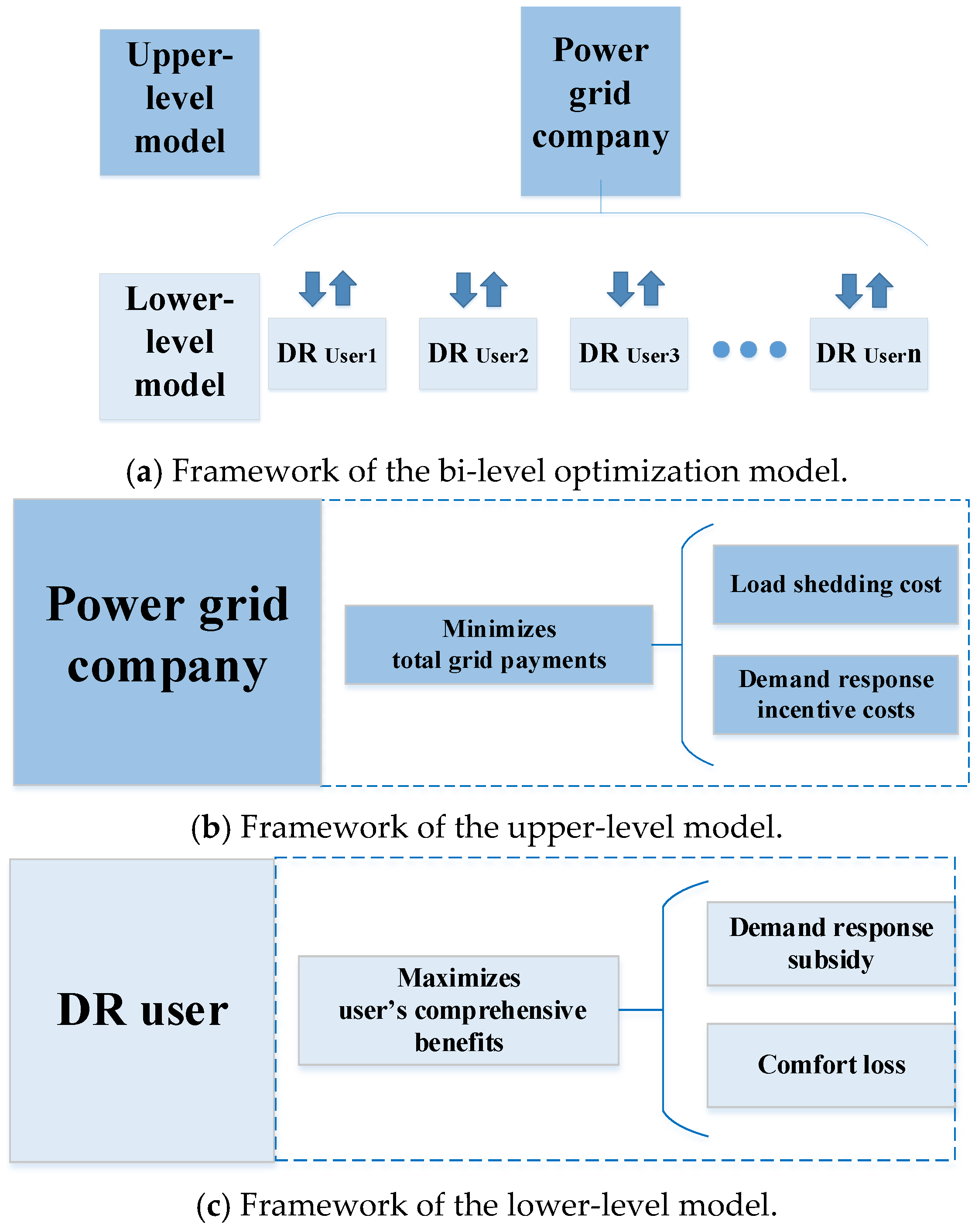
Figure 2 shows the structure of the model. The upper level is a load restoration model. Its goal is to minimize the total payments made by the grid. This model determines the demand response (DR) clearing price for each user. It also calculates the clearing quantity for each user. These values are then passed to the lower level of the model. The lower level is a response decision model. Its goal is to maximize the comprehensive profits of each user participating in DR. This model determines the actual response quantity for each user. It also calculates the step incentive coefficient. These results are then fed back to the upper level of the model. This iterative process continues until an optimal solution is found that balances the interests of both parties.
3.1. Upper-Level Model
The load restoration model aims to alleviate the supply–demand imbalance by optimizing energy allocation. This model allocates energy based on the extent of user participation in DR and the currently available generation capacity. The load shedding penalty is incurred when the actual load allocation is lower than the demand.
In addition, compared with only using load recovery or reliability as the objective function, using cost as the objective function in Equation (7) can more effectively coordinate the upper and lower levels of models and achieve the comprehensive optimization of the power system at the economic and technical levels.
Therefore, the objective function of the upper-level model is to minimize the sum of load shedding penalty costs and DR costs, as shown in Equation (7).
where
represents the set of users connected to node
n;
T is the set of time periods;
and
denote the load shedding penalty cost and the DR incentive cost, respectively, as shown in Equations (8) and (9):
where
represents the penalty of load shedding per MW;
represents the load quantity;
represents the priority of load
j;
is the energy supply ratio, representing the ratio of the load supplied by the system to the user’s demand;
is the clearing price of DR;
is the incentive coefficient for user
j;
is the actual response quantity.
The constraints of the upper level are as follows:
- (1)
Node power balance constraint
where
and
represent the set of generators and users connected to node
n, respectively;
and
represent the active and reactive power of the generator at node
n, respectively;
and
represent the active and reactive power injection at node
n, respectively.
where
and
are the voltage magnitude and phase angle of node
n, respectively;
and
represent the active and reactive power flowing through line
n-
m;
,
;
and
are the resistance and reactance of line
n-
m.
- (3)
Security constraint
To ensure the safe operation of the system, the voltage at each node and the power flow on each branch should be limited within a specific range:
where
,
and
,
represent the upper and lower limits of active and reactive power on line
n-
m, respectively;
and
represent the upper and lower limits of voltage at node
n.
3.2. Lower-Level Model
The subsidy for users participating in DR is determined based on their actual electricity reduction. The reduction affects users’ power usage arrangements and lowers their comfort level. The lower-level model considers two main factors. First, it looks at the subsidies for user participation in DR. Second, it takes into account the comfort loss experienced by users. The goal of this model is to maximize overall profit. Additionally, it aims to optimize the actual response electricity. The objective function and related constraints are as follows:
where
represents the comprehensive profit of user
j participating in DR;
denotes the DR subsidy received by the user;
and
are the upper and lower limits of the response quantity for user
j, respectively.
The comfort loss is related to the user’s willingness and ability to respond: the desire to respond can be represented by the user’s response quantity under unit incentive subsidy; the ability to respond depends on the user’s energy dependency and energy usage. As the amount of electricity reduction increases, the user’s comfort loss also increases. This means that there is a positive correlation between electricity reduction and comfort loss. Additionally, the increase in comfort loss is marginal. Therefore, the comfort loss can be expressed using the following quadratic function:
where
is the comfort loss of user
j participating in DR;
and
are the comfort loss coefficients of user
j participating in DR;
is the actual response quantity of user participation in DR.
The comfort loss coefficient can be adjusted according to the urgency of users’ electricity demand under varying weather and temperature conditions. For example, electricity demand significantly increases when users face urgent production orders. At this time, reducing electricity usage may lead to substantial losses, thereby lowering their willingness to participate in DR, which is reflected in the expression of comfort loss as a higher comfort coefficient. Additionally, the maintenance and repair of electrical equipment can also affect their comfort during the actual response phase. Therefore, comfort loss can effectively reflect the urgency of users’ electricity demand.
The loss of users’ electrical comfort indicates users’ satisfaction with electricity and also reflects the response cost of users’ participation in DR. Users have the most optimal value for power consumption. Deviation from this value will reduce users’ comfort degree of power consumption, and the loss of comfort degree has a marginal effect. Therefore, a quadratic function can be used to represent users’ comfort loss.
The electric comfort of different types of users is quite different. This paper estimates the comfort loss function based on the historical reporting results of users in the DR market. This estimation method assumes that a user’s quotation in the DR market is not lower than the marginal value of its response cost, as shown in
Figure 3, where
,
,
and
, respectively, represent the declared price and declared volume of user
j’s first and second participation in the DR market. For the convenience of explanation, only the first two quotations of users are considered in the figure, and the estimation method is similar in the case of multiple quotations. There are four situations:
- (1)
and
. It means that the price and quantity of user
j’s second declaration are less than those of user
j’s first declaration. Under the condition of user rationality, it can be considered that the marginal cost of user response on
is not higher than
, and the marginal cost of user response on
is not higher than
. Therefore, the piecewise linear function composed of red and yellow line segments in
Figure 3a can be used to approximate the comfort loss function of user
j.
- (2)
,
. It means that the price of user
j’s second declaration is less than that of the first, but the quantity of declaration is greater than that of the first. Under the condition of user rationality, it can be considered that the marginal cost of the user’s response on
is not higher than that of
. Therefore, the linear function represented by the red line segment in
Figure 3b is used to approximate the comfort loss function of user
j.
- (3)
When in situations , or , , the same applies.
Figure 3.
Estimation diagram of comfort loss function.
Figure 3.
Estimation diagram of comfort loss function.
4. Iterative Mixed-Integer Load Restoration Solver
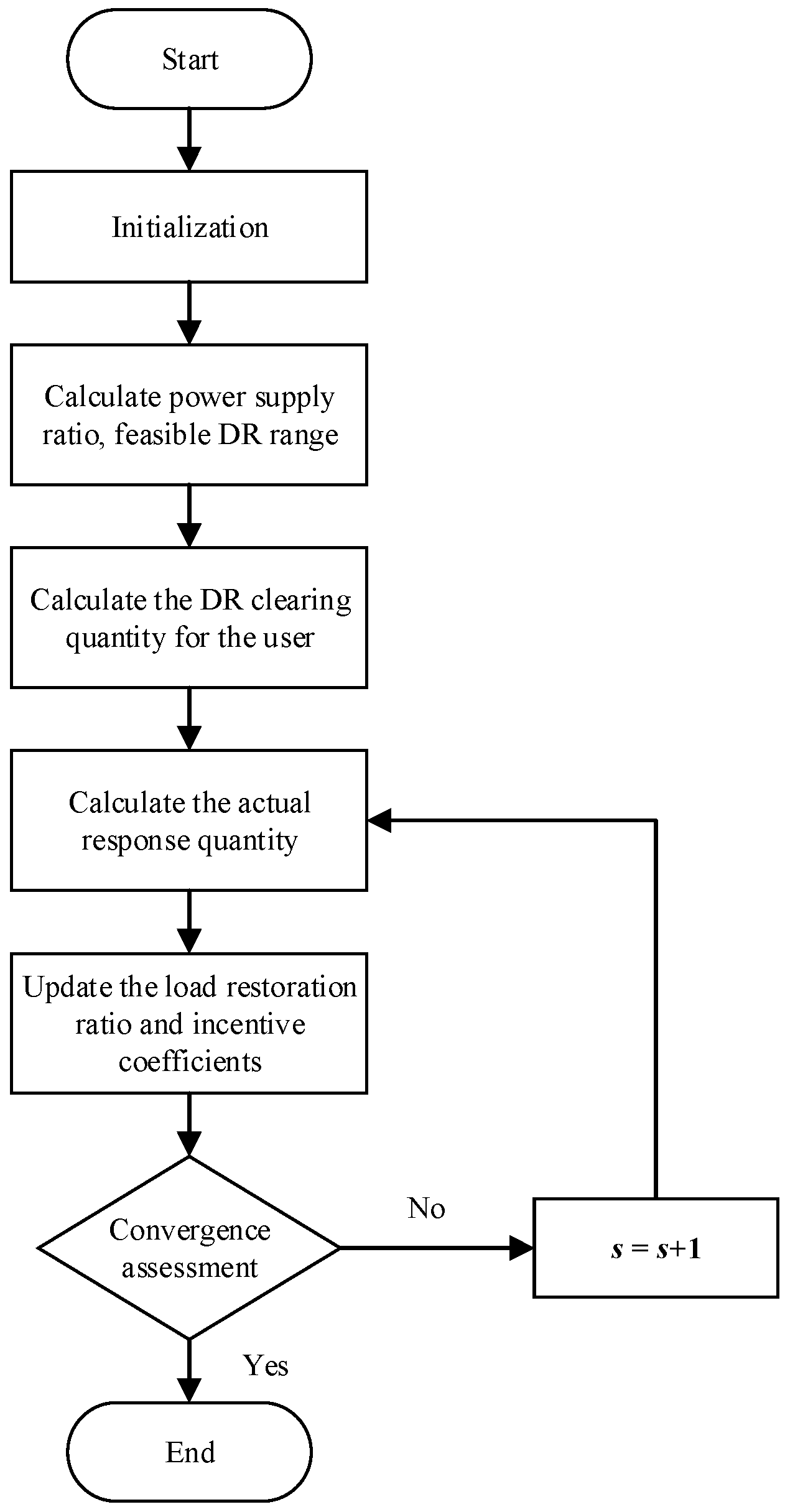
The proposed load restoration model (1)–(18) is a mixed-integer nonlinear programming problem. The solution complexity stems from the coupling relationship between the upper- and lower-level models. Additionally, the objective function and constraints exhibit nonlinear characteristics. Rapid load restoration after extreme disasters imposes higher requirements on the computational efficiency. To address this issue, an iterative mixed-integer load restoration solver is proposed. This solver coordinates the optimization processes of the upper- and lower-level models, gradually approaching the optimal solution. The flowchart of the proposed solution algorithm is shown in
Figure 4. In addition,
Appendix A had given the convergence proof of the algorithm.
- (1)
Initialization. The parameters, including the tiered incentive intervals , initial tiered incentive coefficients , and user priority levels , are set. The iteration counter is initialized as .
- (2)
The power supply ratio and maximum demand response are calculated. Neglecting the impacts of DR (i.e., setting ), the optimization problem in Equations (7)–(16) is solved to obtain the power supply ratio and maximum demand response .
- (3)
The clearing quantity of DR is calculated. A piecewise linear function is used to fit the relationship between the DR clearing price and the total clearing quantity , as shown in Equation (19).
Substituting the fitting results into Equation (9) yields the following:
where
k and
b are the fitting parameters;
denotes the clearing quantity of user
j which satisfies the following relationship:
where
denotes the maximum DR capacity that user
j can provide, as obtained in Step (2).
In Equation (20), two simplifications are carried out: (1) the incentive coefficients is neglected; (2) the actual DR quantity is replaced by the clearing quantity.
- (4)
The actual DR quantity is calculated. In the s − 1 iteration, the tiered incentive coefficients , the DR clearing quantity , and the clearing price are used as inputs to solve optimization problems (9), (17), (18), (22), (24) and (26). The actual DR quantity is determined by solving a quadratic programming problem.
Additionally, the functions in Equation (3) are linearized as follows. A new auxiliary integer variable
is introduced. Equation (3) is then equivalent to the following constraints.
Note that
,
, and
are known parameters in Equations (22)–(25). Furthermore, Equation (23) can be expressed as follows:
where
denotes the maximum value of
.
- (5)
The energy supply ratio and tiered incentive coefficients are updated. Based on the actual DR quantity and the clearing price , the optimization problem (4), (5), (7)–(16), (22), (25) and (26) is solved. Then, the updated energy supply ratio and tiered incentive coefficients are calculated.
- (6)
Next, convergence check is carried out. The proposed solution algorithm stops when the difference in the energy supply ratio in two consecutive iterations is less than a certain tolerance ε, as shown in Equation (27). If convergence is not achieved, we return to Step (4) for further iteration.
where
denotes the energy supply ratio of user
j at time
t in the
s-th iteration, and
denotes the prescribed restoration parameter.
5. Case Study
5.1. Basic Data
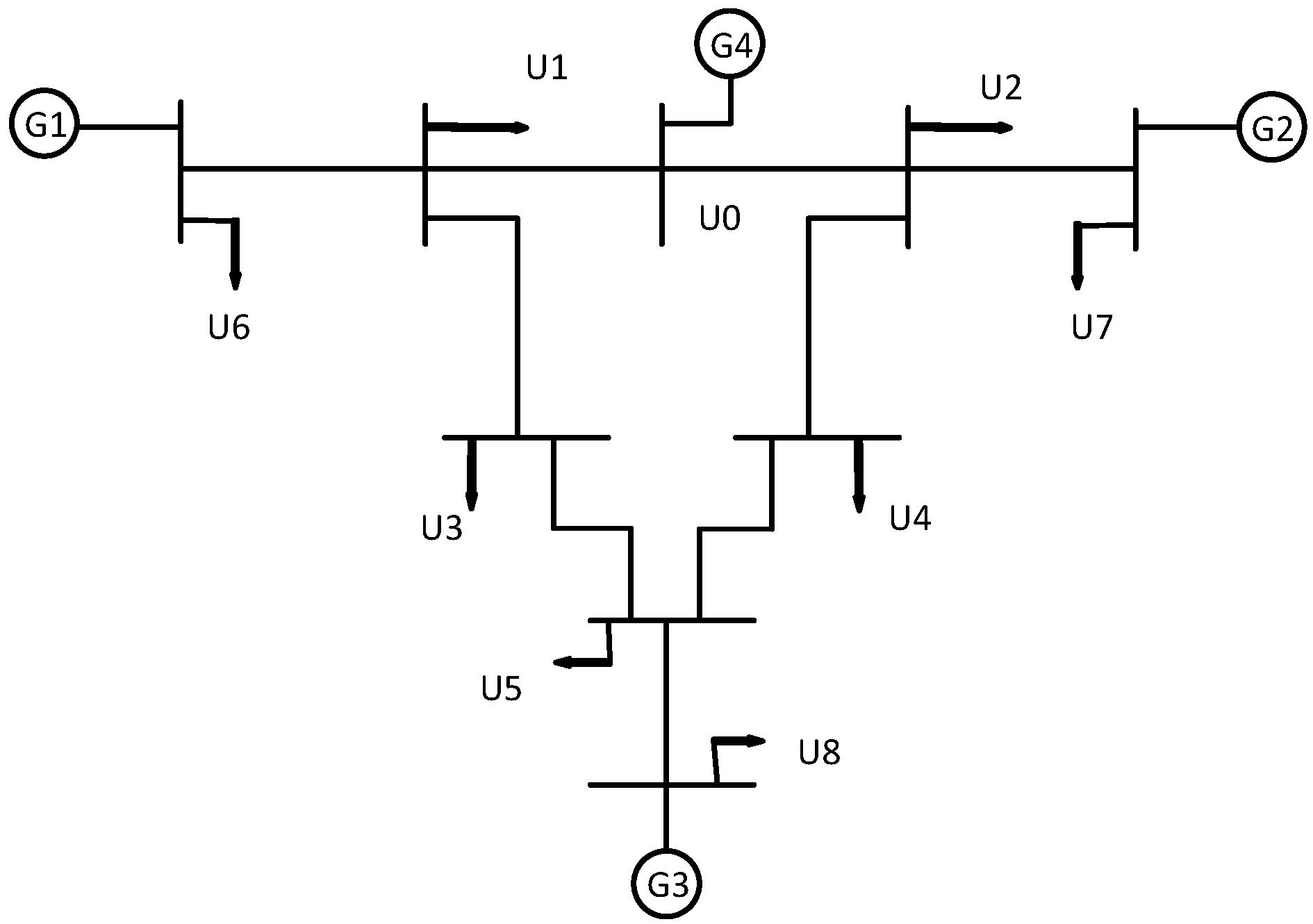
This section validates the effectiveness of the proposed method using a modified IEEE 9-bus system. The system includes 8 users (U1–U8) and 3 thermal power units.
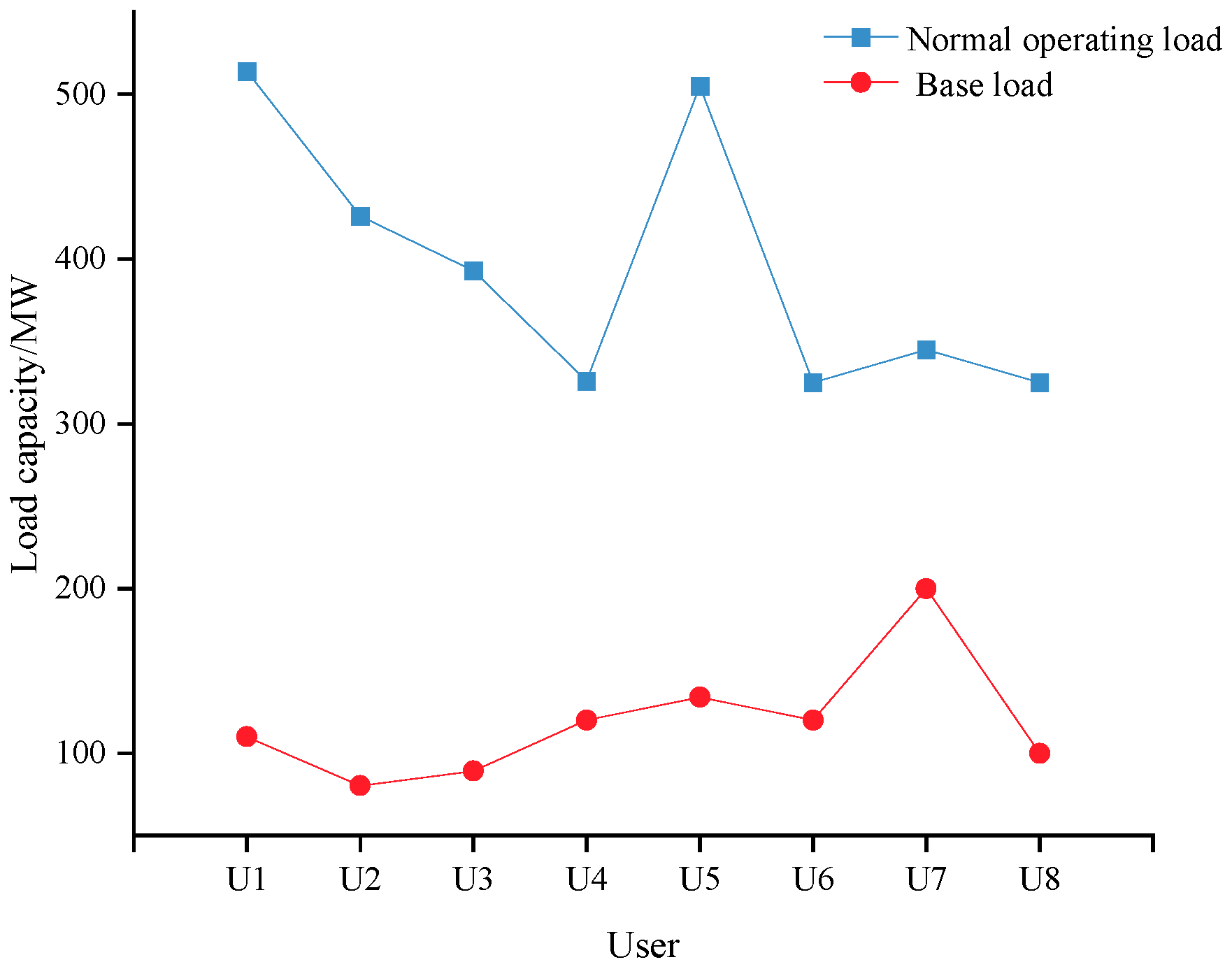
Figure 5 shows the topology of the modified IEEE 9-bus system, where U0 is the reference node. The normal and basic load of each user are shown in
Figure 6. The load-shedding penalty coefficient was 137.56 CNY/MWH [
21]. The priority coefficient of users can be divided into three levels: 100, 10, and 0.2 [
22], which is listed in
Table 1. The thermal units, G1, G2, G3, and G4, have installed capacities of 646 MW, 652 MW, 687 MW and 1000 MW, respectively. The price–quantity relationship was estimated by fitting historical data. The data used were from the previous 10 DR clearing quantities and clearing prices, as shown in
Figure 7. It was assumed that an extreme disaster causes the shutdown of thermal unit G4, leading to an imbalance between power supply and demand. The prescribed restoration parameter
was set to 0.01.
The case study primarily analyzed variations in user profit, incentive coefficients, actual response quantities, clearing prices, grid payments, and tiered incentive coefficients under different conditions.
Section 5.2 compared the effects of fixed and time-varying step incentive coefficients on the model solution. The effectiveness of the symmetrical DR incentive mechanism in reducing the cost of the grid and enhancing the profits of users were verified.
Section 5.3 evaluated the effects of different tiered incentive intervals on user’s profit and the cost of the grid.
The simulation program was run on a PC with an Intel i5-9300H processor, 2.40 GHz, and 8.00 GB RAM. The commercial solver, CPLEX12.9, under Python3.7 environment, was used to solve the model proposed in this paper.
5.2. Impacts of Fixed and Optimized Symmetrical Incentive Coefficients
In this section, the tiered incentive coefficients are set to fixed values (Scenario M1) and optimized values (Scenario M2), as shown in
Table 2.
Figure 8,
Figure 9,
Figure 10 and
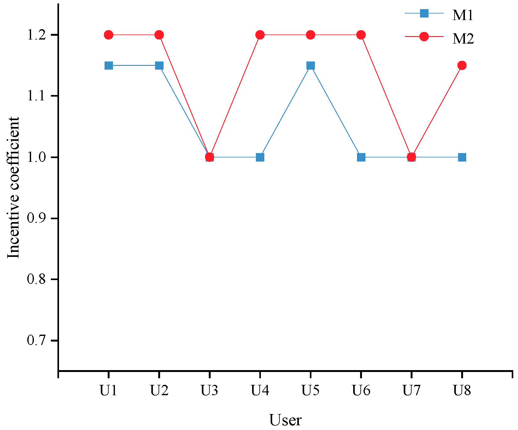
Figure 11 show the incentive coefficients, clearing quantity, actual response quantities, and profits. Compared with Scenario M1, the incentive coefficients of users U1, U2, U4, U5, U6 and U8 are higher in Scenario M2, as can be seen in
Figure 8. The incentive coefficients of users U3 and U7 remain the same in both scenarios. Further comparison of the data in
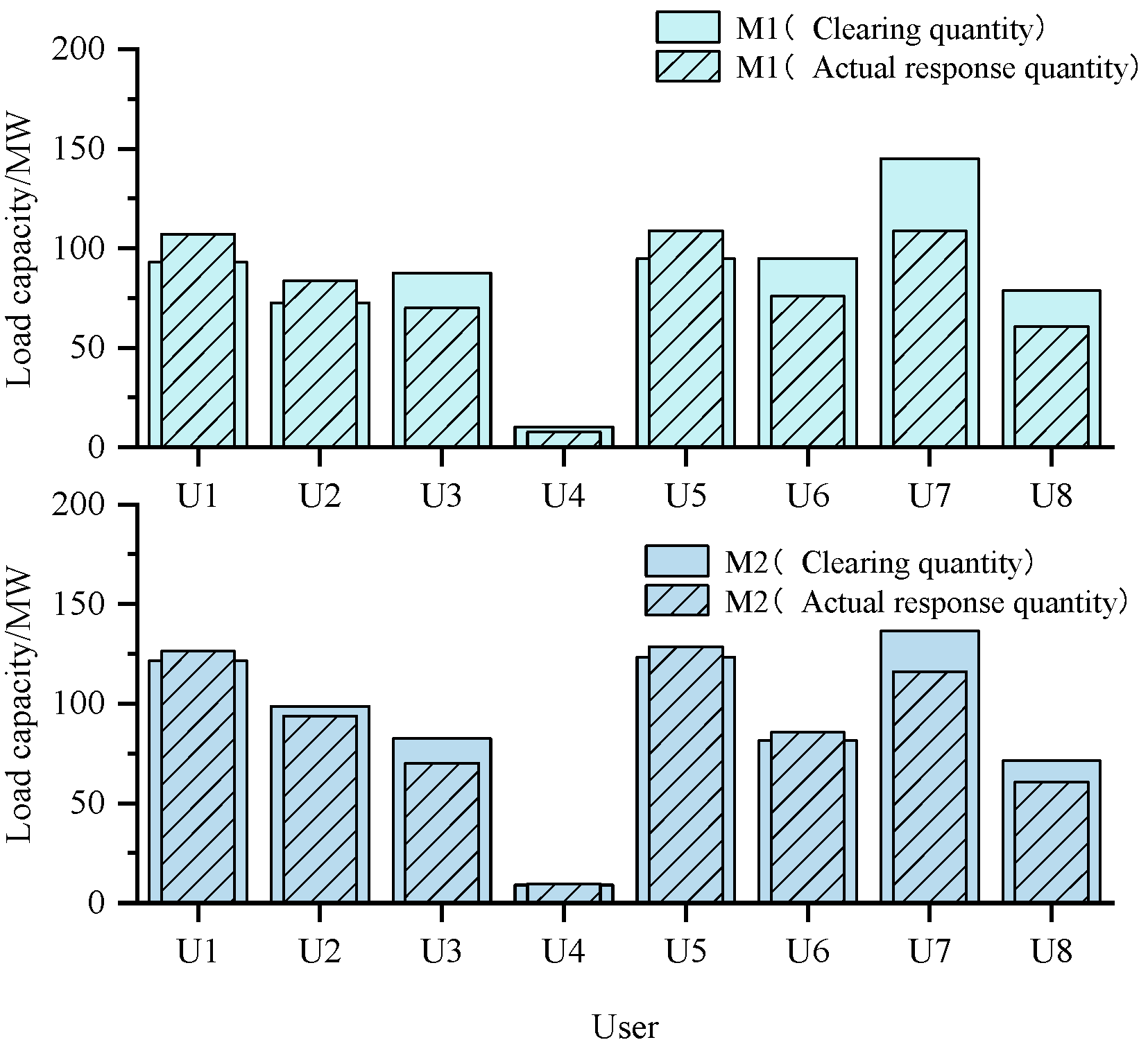
Figure 9 reveals the following: In Scenario M2, the incentive coefficients of users U1, U2 and U4–U6 all reach a peak of 1.2. This indicates that U1, U2 and U4–U6 show a high degree of enthusiasm for participating in DR. Their actual response quantities are almost equal to the cleared quantities. The incentive coefficients of users U3 and U7 are the lowest, at only 1.0. Their actual response quantities are significantly lower than the clearing quantities. In Scenario M1, the incentive coefficients of all users are maintained at a low level. Comparison analysis of
Figure 9 shows the following: a large deviation exited between the actual response quantities and clearing quantities of users U1–U8. This situation was not conducive to the load restoration. By comparing the deviations between actual response quantities and clearing quantities, it is found that the optimized symmetrical incentive mechanism can significantly reduce this deviation. Therefore, the proposed model motivated users to actively participate in DR. This is beneficial for the rapid restoration of system load under extreme conditions.
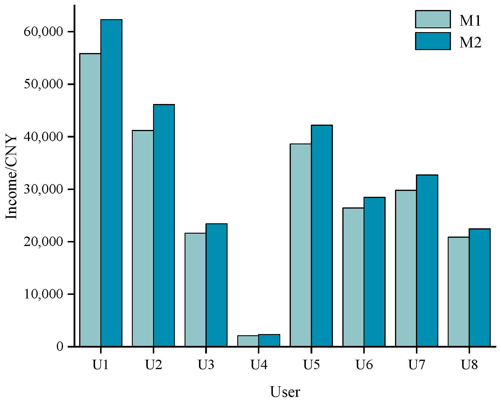
As can be seen in
Figure 10, the profits of each user in Scenario M2 are generally higher than those in Scenario M1. Additionally, from the perspective of the power grid, the costs required to be paid in scenarios M1 and M2 are CNY 3.466 million and CNY 3.638 million. Although the cost of power grid increases slightly, it balances the interests of the power grid and load and can encourage users to actively participate in demand response.
Meanwhile, the unit price of DR clearing also increased from 3.676 CNY/kW in Scenario M1 to 3.692 CNY/kW in Scenario M2. It can be concluded that the proposed symmetrical DR incentive mechanism not only enhances users’ enthusiasm for participating in DR, but also promotes the rapid restoration of load under extreme conditions. The users’ profit was increased. Moreover, the costs that the power grid incur was significantly reduced. A win-win situation was achieved.
In summary, the symmetrical DR incentive mechanism was more effective than the fixed symmetrical incentive mechanism. It was better at mobilizing users’ enthusiasm for participating in DR. Additionally, it is more effective in promoting the rapid restoration of power grid load under extreme conditions.
5.3. Impacts of Tiered Incentive Ranges Profit
By setting different tiered incentive ranges, data on user profit and the cost of the grid under different scenarios (N1–N7) were obtained. The impacts of different tiered incentive ranges on the profit of both the power grid and users were analyzed. Seven types of tiered incentive ranges (with intervals of 0.08, 0.10, 0.12, 0.14, 0.16, 0.18 and 0.20, respectively) were mainly considered, as shown in
Table 3.
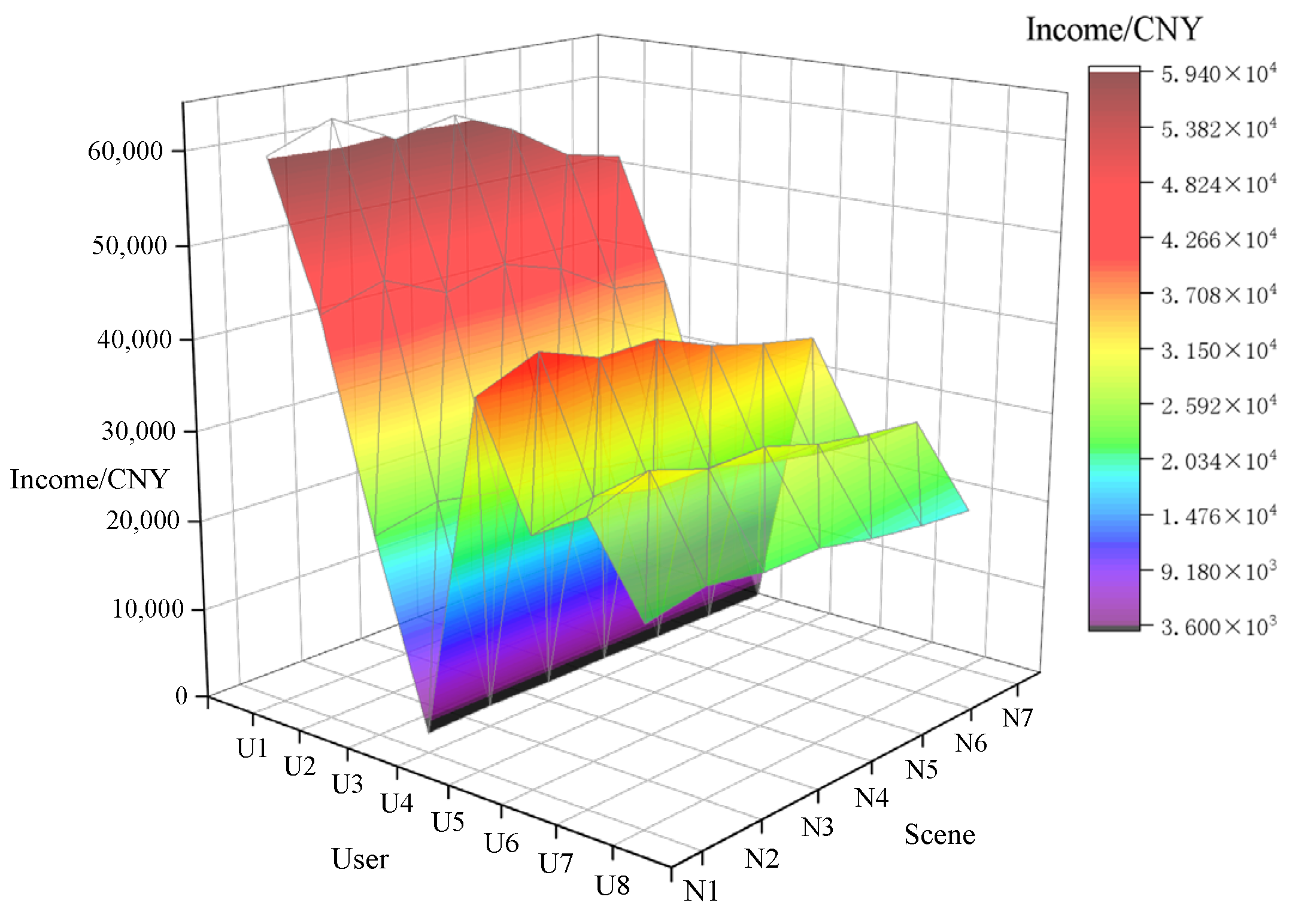
Figure 11 shows the profit of each user under the 7 scenarios. It can be seen that the profits of each user were maximized in Scenario N2 (the tiered incentive range is 0.10). Conversely, the profits of each user are minimized in Scenario N7 (the tiered incentive range is 0.20).
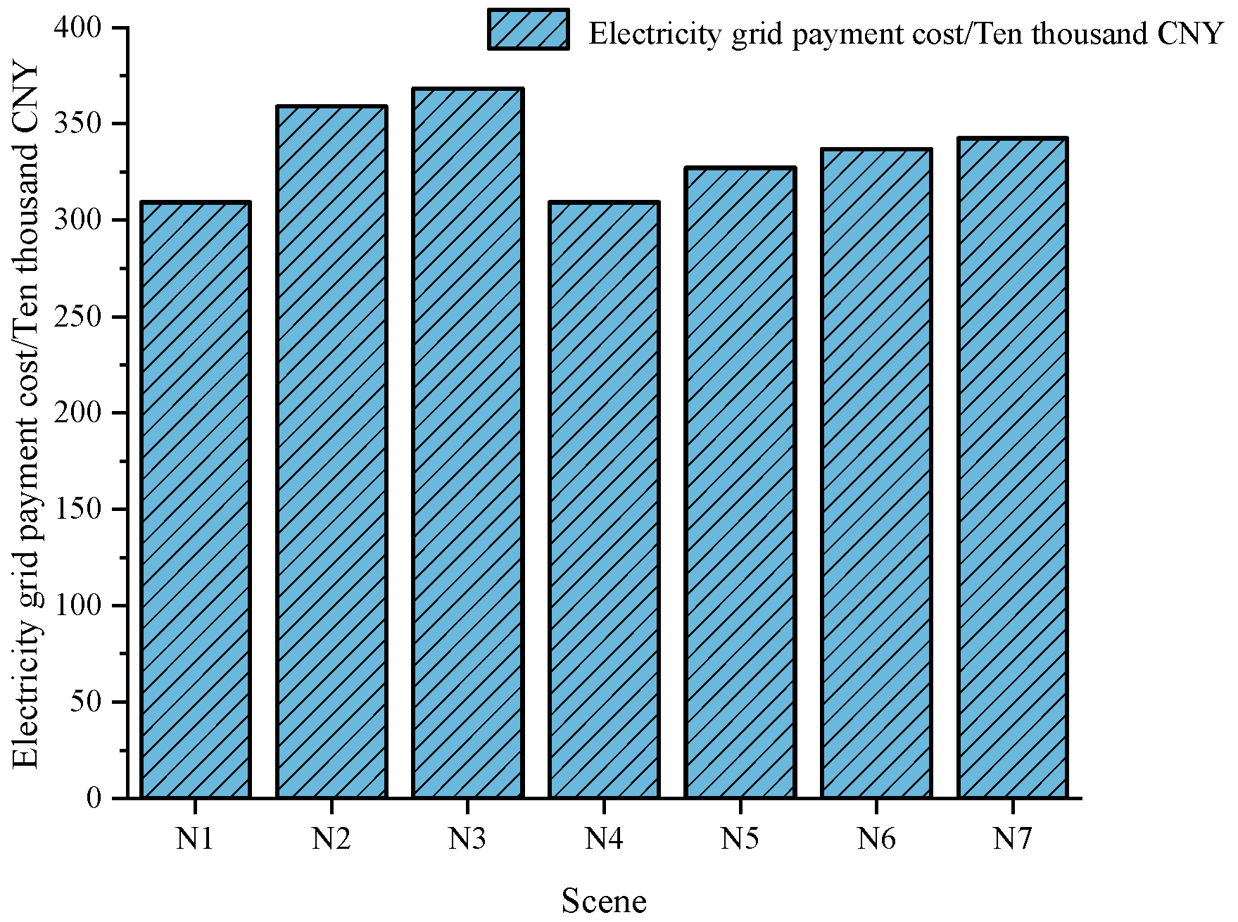
Figure 12 shows the costs that the power grid needs to pay. As can be seen in
Figure 12, the cost paid by the power grid was minimized in Scenario N4, at approximately CNY 3.093 million. In contrast, the cost paid by the power grid was maximized in Scenario N3, which was CNY 0.591 million more than in Scenario N4. Therefore, it was the least favorable scenario for the power grid. Overall, as the interval of the tiered incentive range increases, the cost that the power grid needs to pay tended to rise.
Therefore, selecting the tiered incentive range was crucial for the profit of both the power grid and the load side. An optimal choice can only be made after comprehensively balancing the profit of both parties.
5.4. Discussion
- A.
Reliability of DR under emergency scenarios
The core research objective of this paper is to verify whether demand response can effectively promote the rapid recovery of load in extreme disaster scenarios. The experimental results show that although there is a certain deviation between the actual response of some users and the clearing amount, the users’ participation in demand response significantly reduces the power supply pressure of the grid. Therefore, even if other flexible resources are included in the unified modeling system, demand response can still play an active and effective role in the load recovery process.
- B.
The practical challenges of implementing the symmetrical incentive mechanism in real-world DR programs
- (1)
In reality, the symmetrical incentive mechanism in the implementation of load recovery plan under extreme disasters faces many practical challenges. From the information level, the destruction of communication facilities caused by disasters leads to difficulties in obtaining information, and there is information asymmetry between users and power companies, which affects the rationality and fairness of incentive schemes. In terms of interest coordination, there are conflicts and inconsistencies between different users and between power companies and users, which makes it difficult to meet the needs of all parties and reach consensus at the same time. In terms of mechanism design, the incentive standard is difficult to determine due to various factors, and the incentive method is singular, which cannot effectively attract various users. In the external environment, the relevant laws and regulations are not perfect, and there is a lack of policy support and supervision. At the same time, public opinion is highly concerned about the fairness of the implementation of the incentive mechanism. Once problems occur, they will put enormous pressure on power companies.
- (2)
It is very difficult to collect the comfort parameters of each user, so this paper proposes an estimation method, which has been described in detail in question 4.
- (3)
The unit commitment problem of the model built in this paper is simpler than that of the actual power grid model, mainly because there are fewer Boolean variables in this paper, so the existing equipment in the actual power grid can completely solve the bi-level optimization model proposed in this paper.
6. Conclusions
This paper proposes a symmetrical demand response incentive mechanism, based on a bi-level load restoration optimization model. A bi-level iterative solution algorithm is proposed to balance the profits between grid and load entities. The case studies show the following:
- (1)
The proposed model improved users’ proactive engagement in the DR by dynamically correlating response hierarchy with incentive intensity. The observed participation rate reached 95.34%, showing a 3.38% improvement over conventional fixed symmetrical incentive schemes.
- (2)
From the cost–profit perspective, the cost of power grid measurement increases slightly, while the load-side profit experiences an increase of CNY 23,545.26. During grid stress conditions caused by supply–demand imbalance, the proposed model exhibits dual functionality: optimizing electricity consumption pattern while alleviating operational strain, thereby accelerating load restoration processes.
- (3)
The proposed iterative mixed-integer load restoration solver eliminated the need for solving large-scale mixed-integer nonlinear programming problems. All tested scenarios converged within 1 min, thereby validating the computational efficiency for proposed nonlinear bi-level optimization model.
The model in this paper does not adequately address load uncertainty, as actual power system loads fluctuate, impacting model accuracy and reliability. Additionally, the demand response mechanism faces limitations; many users lack motivation to participate, even with incentives, prioritizing their operational needs over potential economic benefits. This highlights challenges in mobilizing user participation. Future research should focus on user participation uncertainty in DR, considering load fluctuations, and aim to create effective incentive mechanisms to enhance power system efficiency, stability, and reliability, especially after extreme events.


 and
and 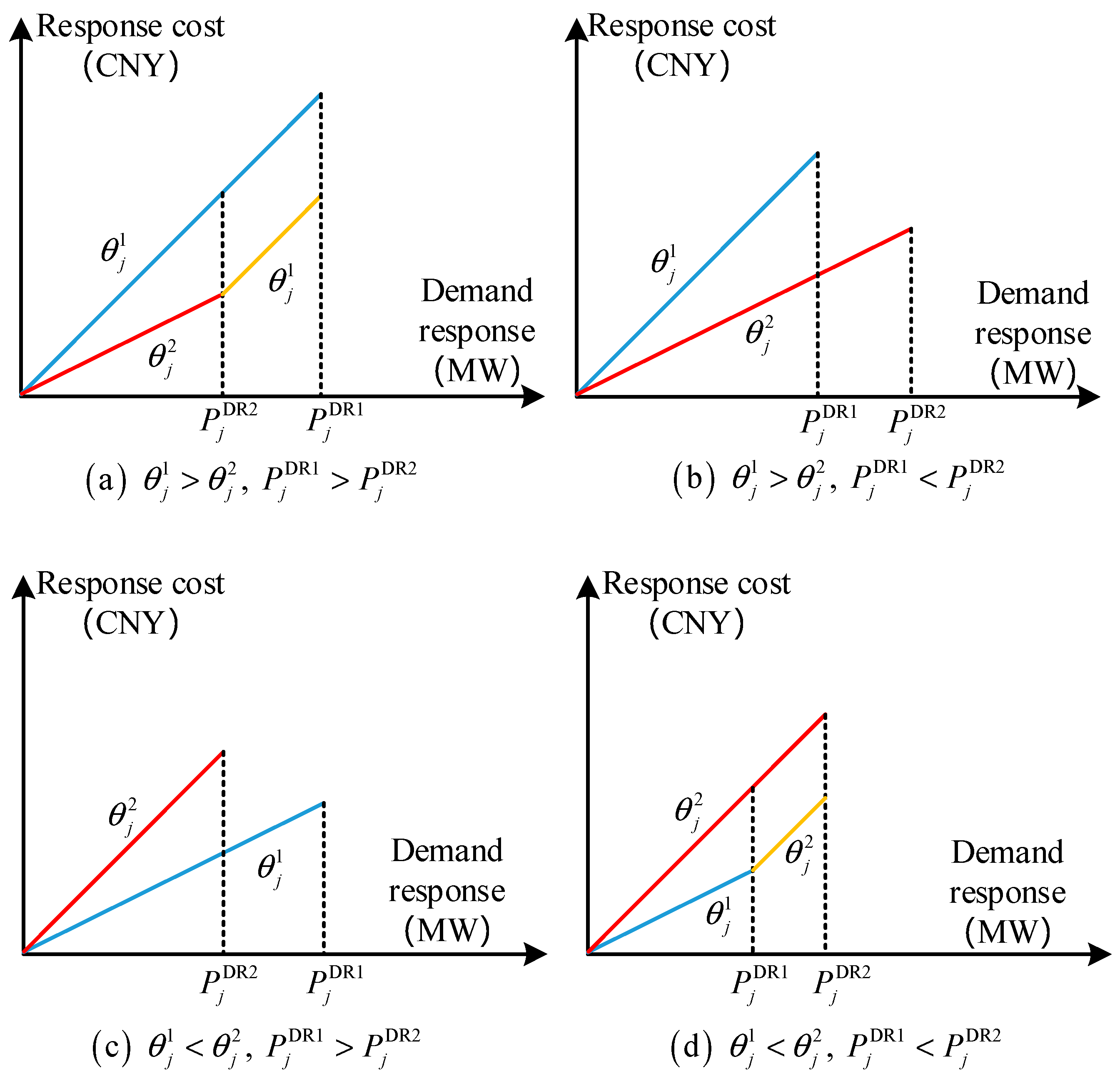


