Online Pre-Diagnosis of Multiple Faults in Proton Exchange Membrane Fuel Cells by Convolutional Neural Network Based Bi-Directional Long Short-Term Memory Parallel Model with Attention Mechanism

Abstract

Proton exchange membrane fuel cell (PEMFC) fault diagnosis faces two critical limitations: conventional offline methods lack real-time predictive capability, while existing prediction approaches are confined to single fault types. To address these gaps, this study proposes an online multi-fault prediction framework integrating three novel contributions: (1) a sensor fusion strategy leveraging existing thermal/electrochemical measurements (voltage, current, temperature, humidity, and pressure) without requiring embedded stack sensors; (2) a real-time sliding window mechanism enabling dynamic prediction updates every 1 s under variable load conditions; and (3) a modified CNN-based Bi-LSTM parallel model with attention mechanism (ConvBLSTM-PMwA) architecture featuring multi-input multi-output (MIMO) capability for simultaneous flooding/air-starvation detection. Through comparative analysis of different neural architectures using experimental datasets, the optimized ConvBLSTM-PMwA achieved 96.49% accuracy in predicting dual faults 64.63 s pre-occurrence, outperforming conventional LSTM models in both temporal resolution and long-term forecast reliability.

1. Introduction

In recent years, research on clean energy has become an important direction to alleviate global warming and environmental pollution. Fuel cells can accelerate carbon neutrality, so they have attracted widespread attention [1]. In 2019, fuel cell systems with a total power of more than 130 MW were completed worldwide [2]. Currently, there are more than 10,000 fuel cell electric vehicles (FCEVs) on the road in the United States, while China and Japan reported over 6000 and 3520 FCEVs in operation, respectively [3]. Among all fuel cells, proton exchange membrane fuel cell (PEMFC) has the advantages of zero pollution, low noise, and high efficiency, and is an ideal green energy source [4]. PEMFCs are also widely applied in electric vehicles and green buildings [5,6]. However, during long-term operation, the PEMFC may encounter faults such as flooding [7,8], insufficient air or hydrogen [9], and membrane drying out [10], which lead to performance degradation [11,12], shortened lifetime, and unsustainable commercial applicability [13,14]. Peripheral components such as valves, compressors, and sensors are also required to control the fuel cell stack [15,16]. Therefore, effective fuel cell fault diagnosis and control methods are also important to reduce the operating costs and extend the life of fuel cells.

To directly diagnose the faults of the fuel cell, many methods have been extensively studied by researchers, involving methods such as transparent fuel cells [17], X-ray radiography [18,19], and neutron imaging [20,21]. Although these methods are only suitable for single-unit fuel cells instead of stacks, they can reveal the fault driving mechanism, explore the influence law of parameters, and guide the development of corresponding fault detection models. For example, the voltage of a fuel cell is often used as the basic indicator for fault detection [22]. Nevertheless, as these direct observation methods have practical limitations, such as being only applicable to a single fuel cell unit, the researchers collected data through various types of non-destructive sensors and proposed more practical fault diagnosis methods. Andrej et al. [23] used electrochemical impedance spectroscopy (EIS) to detect faults in flooding and drying. Ren et al. [24] used a semi-empirical equivalent circuit model to study the changes in mass transfer during water flooding by using an impedance-based zero-phase ohmic resistance measurement method. Khaled et al. [25] proposed a theoretical model approximating cell potential, relative humidity, and impedance, determining the state of PEMFC is determined by fuzzy logic clustering. Chen et al. [26] developed a multi-input and multi-output (MIMO) fuzzy control method, which is proposed for the hydrothermal management of PEMFC. Pan et al. [27] proposed a modified open-loop PD-ILC method to analysis the fault of PEMFC and control the purge. The main drawback of the above methods is that the researchers, based on their own experience, need to create models to determine the working state and fault type of the fuel cell.

It is not reasonable to use a local linear model to estimate all fuel cell model nonlinear parameters because different operating conditions cannot be modeled [28,29]. Therefore, the data-driven approach has been widely used in the existing PEMFC fault diagnosis research. Many data-driven fault diagnosis methods have been proposed, such as Gaussian Naive Bayesian, support vector machine, and k-nearest neighbor algorithm [30]. In recent years, neural networks such as deep neural network (DNN) [31], convolutional neural network (CNN) [32], and long short-term memory (LSTM) [7] have been introduced into the field of fuel cell fault diagnosis. These methods enable accurate diagnosis after the water fault of a fuel cell has occurred and can inform the operator. The above-mentioned data-driven methods for fuel cell fault diagnosis are all based on offline data.

However, such an approach requires collecting long periods of operating data, can only obtain past diagnostic results, and cannot be used to detect sudden faults or help the operator make timely adjustments. If the recoverable faults, such as flooding and dry out, can be predicted in advance, they can be effectively cured by adjusting the cooling system, temporarily changing the current density or input air temperature and humidity, or purging the electrodes [33,34]. Kim et al. [35] built a pre-diagnostic system using LSTMs and CNNs. This model can pre-diagnose flooding based on past to present data, although it is running offline and it only concerns one type of fault, which is about water inside the fuel cell.

The critical limitation of existing predictive approaches lies in their inability to perform real-time multi-fault anticipation. Unlike the single type of prediction described above, many applications in neural networks in other fields require the recognition of multidimensional sequences. A 1-D CNN-based bi-directional LSTM parallel model with attention mechanism (ConvBLSTM-PMwA) was proposed in 2022. Yin et al. [36] created this new structure to achieve Human Activity Recognition, and the results show that this model performs better than the existing CNN and LSTM models.

To bridge this technological gap, this paper proposed the first real-time online prediction framework of fuel cells capable of multi-fault prediction. This paper improves the ConvBLSTM-PMwA model by modifying the CNN channels and updating the model from multiple-input and single-output (MISO) to multiple-input and multiple-output (MIMO). Additionally, it proposes a real-time online fault prediction method to pre-diagnose the type of fuel cell fault and fault occurrence time under different operating conditions.

The main contributions are summarized as follows:

• We use existing sensors to select the input features of the required fault prediction model according to the electrochemical and thermodynamic principles of the fuel cell stack. Therefore, our method does not require installing embedded sensors in the FC stack.
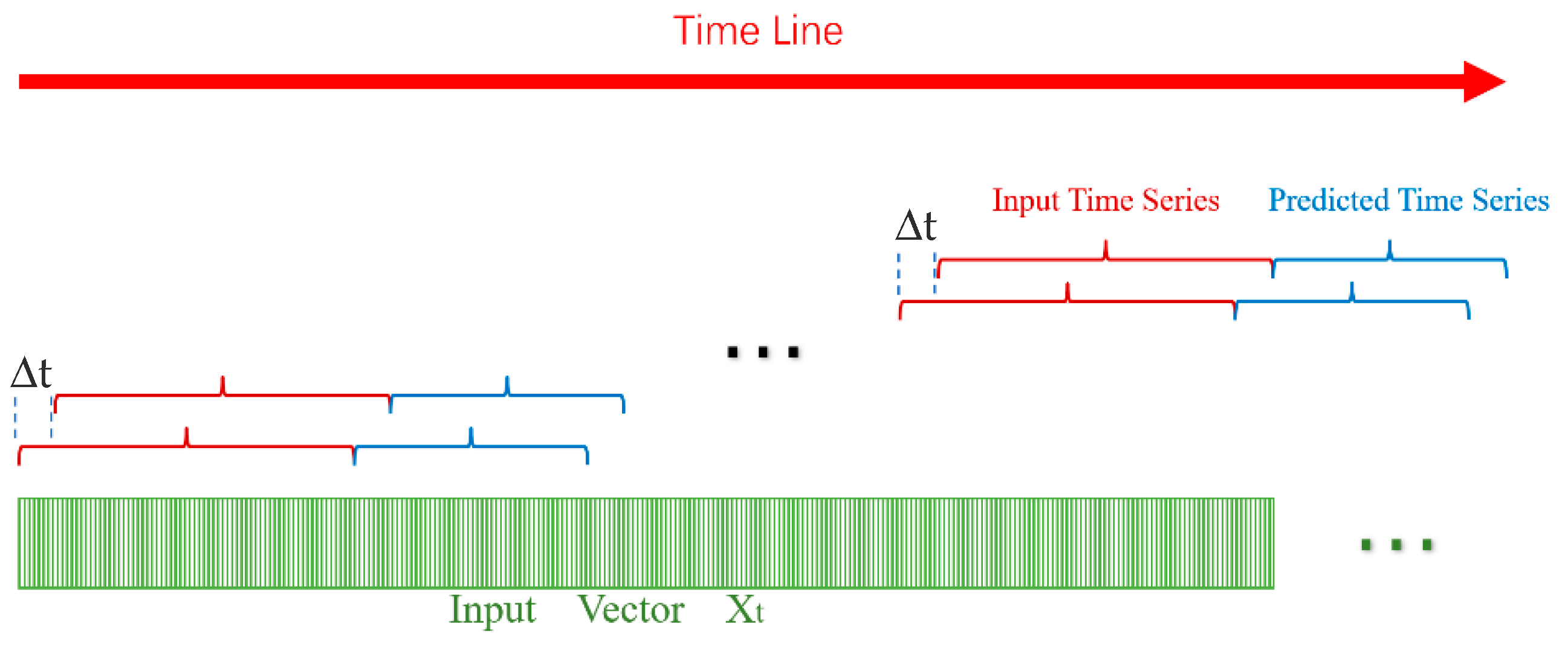
• We consider the load change and simulate the working state of FC under real variable working states. By iteratively updating the input data tensor every second, the model can respond to the monitoring data online in real time, reducing data latency from minutes to 1 second compared to conventional methods.
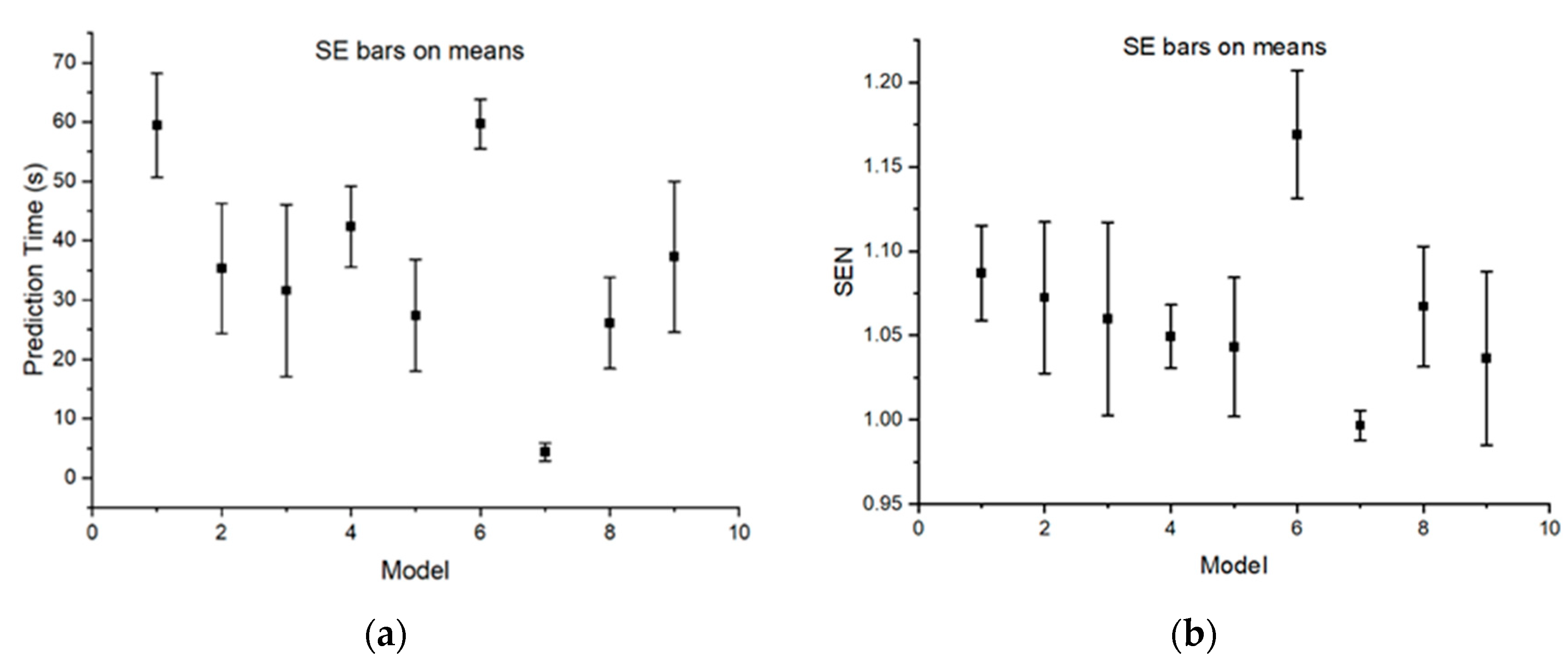
• We evaluate the performance of two different neural network models, LSTM and ConvBLSTM-PMwA, using the FC real fault dataset. We compare the impact of different network architectures, hyperparameters, and target future time on prediction performance. We also compare the prediction effects of different models by prediction times, their coefficient of variations, accuracies, and model sensitivities.

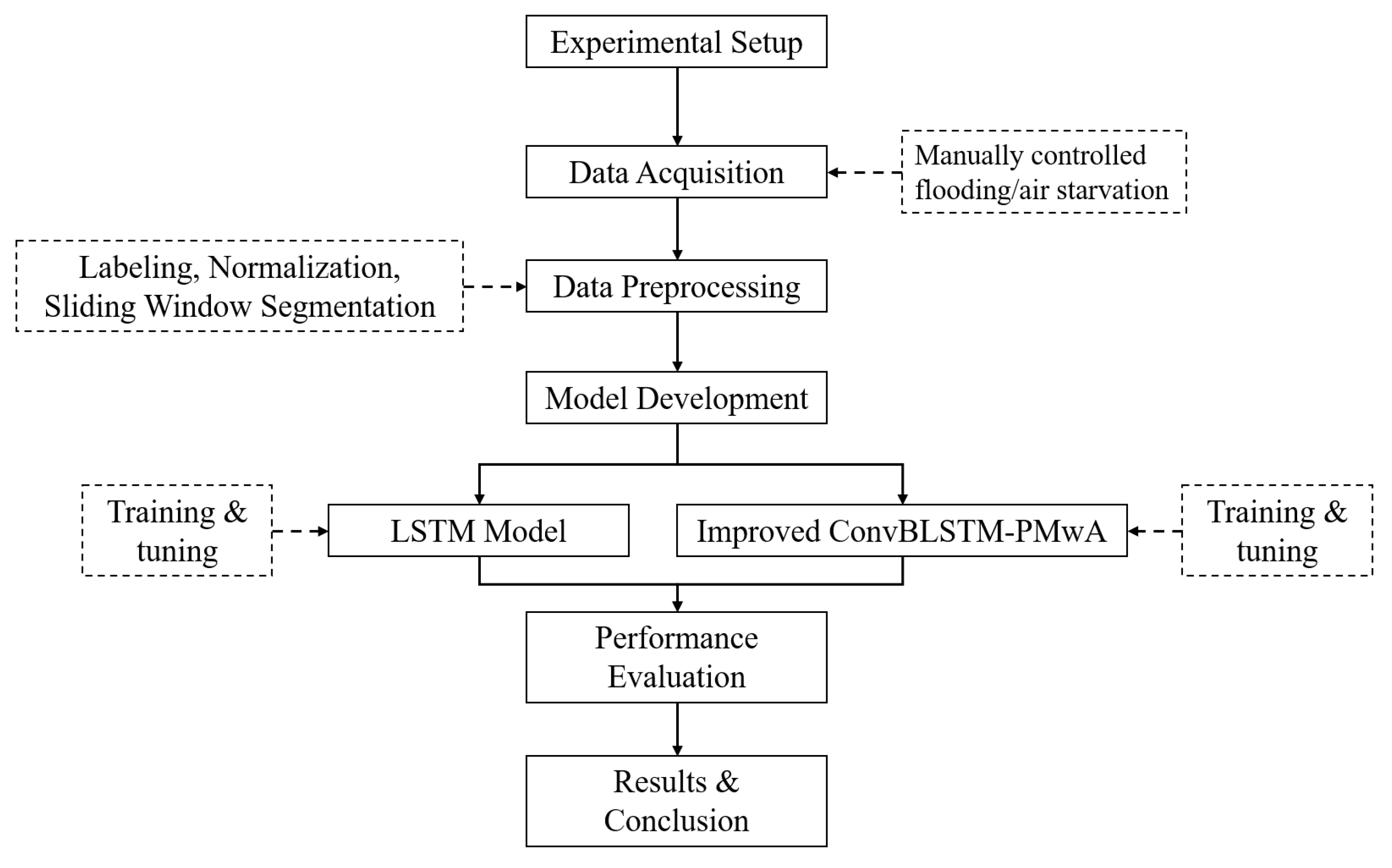
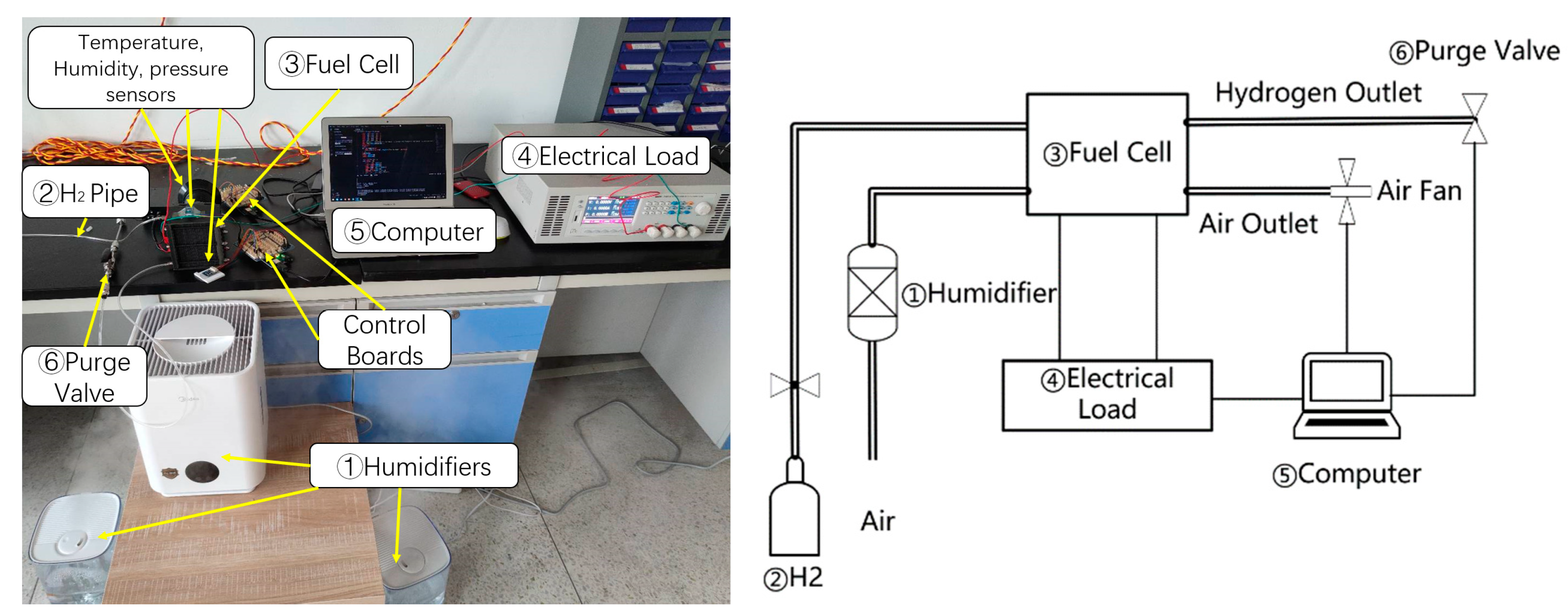
2. Method

Figure 1 shows the block diagram, visualizing the workflow of this study.

The main process of this study is listed below:

• Collect data of PEMFC under normal working conditions and different fault conditions through experiments, and then preprocess and manually label the data;
• Build LSTM and ConvBLSTM-PMwA neural networks, use 70% of the preprocessed sensor data as input and the manually labeled fault indication data as output, and train the neural networks;
• Change the structure and hyperparameters of LSTM and ConvBLSTM-PMwA neural networks, use the remaining 30% of data for testing to select the neural network that can predict the working condition of fuel cell most accurately in the future period of time, and compare the prediction effects.

2.1. Data Marking and Processing

In order to train a neural network model, the data collected by the sensor usually need to be preprocessed. The processing methods in this study include data labeling, data normalization, and data segmentation.

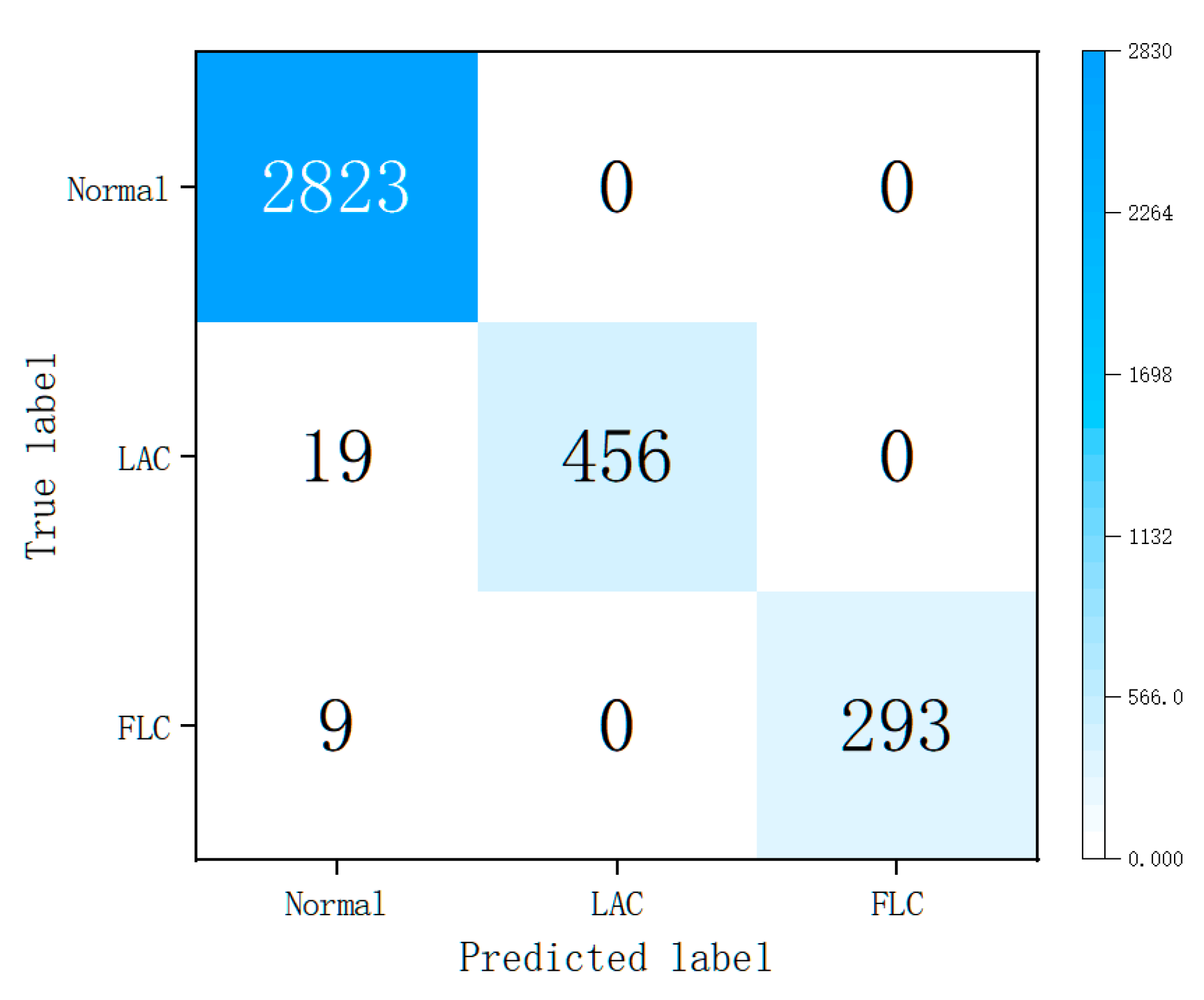
• Data labeling: The data labeling method is marking the training samples into the identified original data. In this study, we conduct multiple independent experiments for flooding and air starvation faults under varying load profiles (e.g., current, dynamic cycles) to generate diverse datasets. We include at least 10 repetitions for each fault type to ensure statistical validity. The data are labeled by adding two different parameters. In the flooding experiment, the normal and stable working states are taken as the standard. During the flooding process, if the output power of the fuel cell is less than 80% of the normal value standard, the marked flooding fault condition (FLC) parameter becomes FLC = 1, and FLC = 0 in other cases. In the air starvation experiment, when we take the normal stable working state as the standard and the output power of the fuel cell is less than 80% of the normal value standard, the marked air starvation condition (LAC) parameter becomes LAC = 1, and LAC = 0 in other cases.
• Data normalization: To mitigate or remove the effect of data range difference, it is often necessary to normalize the raw data, which is a method of adjusting the values of numeric variables in the example dataset to typical scales. This paper uses a relatively simple and effective maximum normalization method. The calculation formula is as follows:

  $$x={\displaystyle \frac{x-\mathrm{m}\mathrm{i}\mathrm{n} \left(x\right)}{\max \left(x\right)-\mathrm{m}\mathrm{i}\mathrm{n} \left(x\right)}}.$$

  (1)
• Data grouping: The data of a neural network is usually divided into two groups, namely the training dataset and the test dataset. The training dataset is used to train the model, and a portion of the data is used as a validation dataset to adjust the training parameters. The test dataset is used to verify the performance of the neural network model.

2.2. Neural Network Models

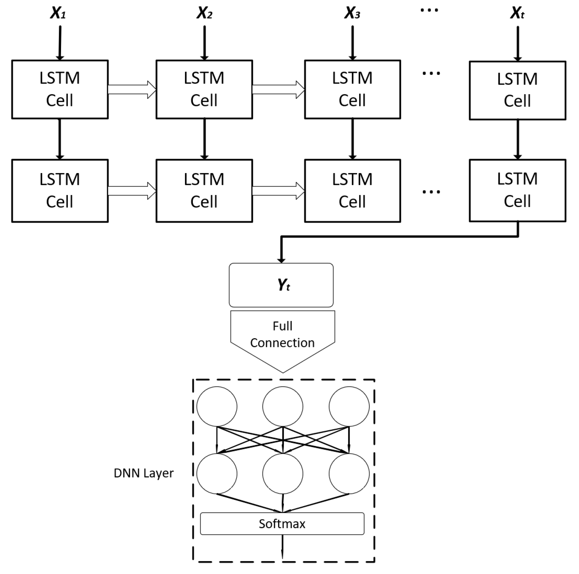
2.2.1. LSTM Neural Network Model

The perceptron is the basic structure of neural networks that are stacked together and takes many inputs while outputting a single value. A perceptron can be represented as follows:

$$y=g(w^{T}x+b).$$

(2)

The idea is to use weight $w$ to represent the importance of one input $x$. $y$ is output, $g$ is activation function, and $b$ is bias.

Based on the perceptron, many new complex neural networks have been created. For example, LSTM is a recurrent neural network that solves the problem of vanishing gradients by reducing the occurrence of information lost from past hidden states. The forget gate erases part of long-term memory through an element-wise multiplication operation while new memory components are added to input gates. The formula for a single step of the LSTM unit is as follows:

$$f_t=\sigma (W_{xf}^T{x}_t+W_{hf}^T{h}_{t-1}+b_f)$$

(3)

$$i_t=\sigma (W_{xi}^T{x}_t+W_{hi}^T{h}_{t-1}+b_i)$$

(4)

$$o_t=\sigma (W_{xo}^T{x}_t+W_{ho}^T{h}_{t-1}+b_o)$$

(5)

$$g_t=tanh(W_{xg}^T{x}_t+W_{hg}^T{h}_{t-1}+b_g)$$

(6)

$$c_t=f_t\circ c_{t-1}+i_t\circ g_t$$

(7)

$$y_t=h_t=o_t\circ \mathrm{t}\mathrm{a}\mathrm{n}\mathrm{h} \left(c_t\right),$$

(8)

where $f_t$, $i_t$, and $o_t$ are the gate controllers at time step $t$, $g_t$ is new information at time step $t$ and $c_t$ are the cell long-term memory state, $y_t$ is the cell output at time step $t$, $h_t$ is hidden short-term state, $W$ is the weight matrix, and $b$ is the bias.

The structure of the neural network is shown in Figure 2.

The input vector, shown above as function (5), is delivered into the LSTM unit. The output vector is as follows:

$$Output Vector=\left[{\left[-r_{t\_FLC}-\right]}^T,{\left[-r_{t\_LAC}-\right]}^T\right].$$

(9)

Here, $r_{t\_FLC}$ is the probability of flooding fault at time t and $r_{t\_LAC}$ are the probability of air starvation at time t. Here, we set the $T=60\mathrm{s}$ as the time window in our study. The target prediction time used to determine accuracy is 60 s in the future of the current data time.

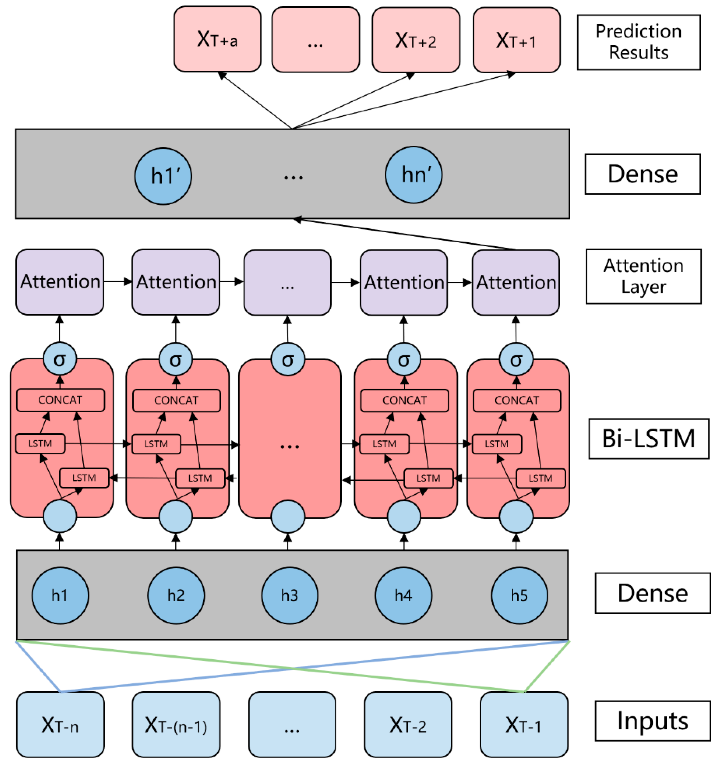
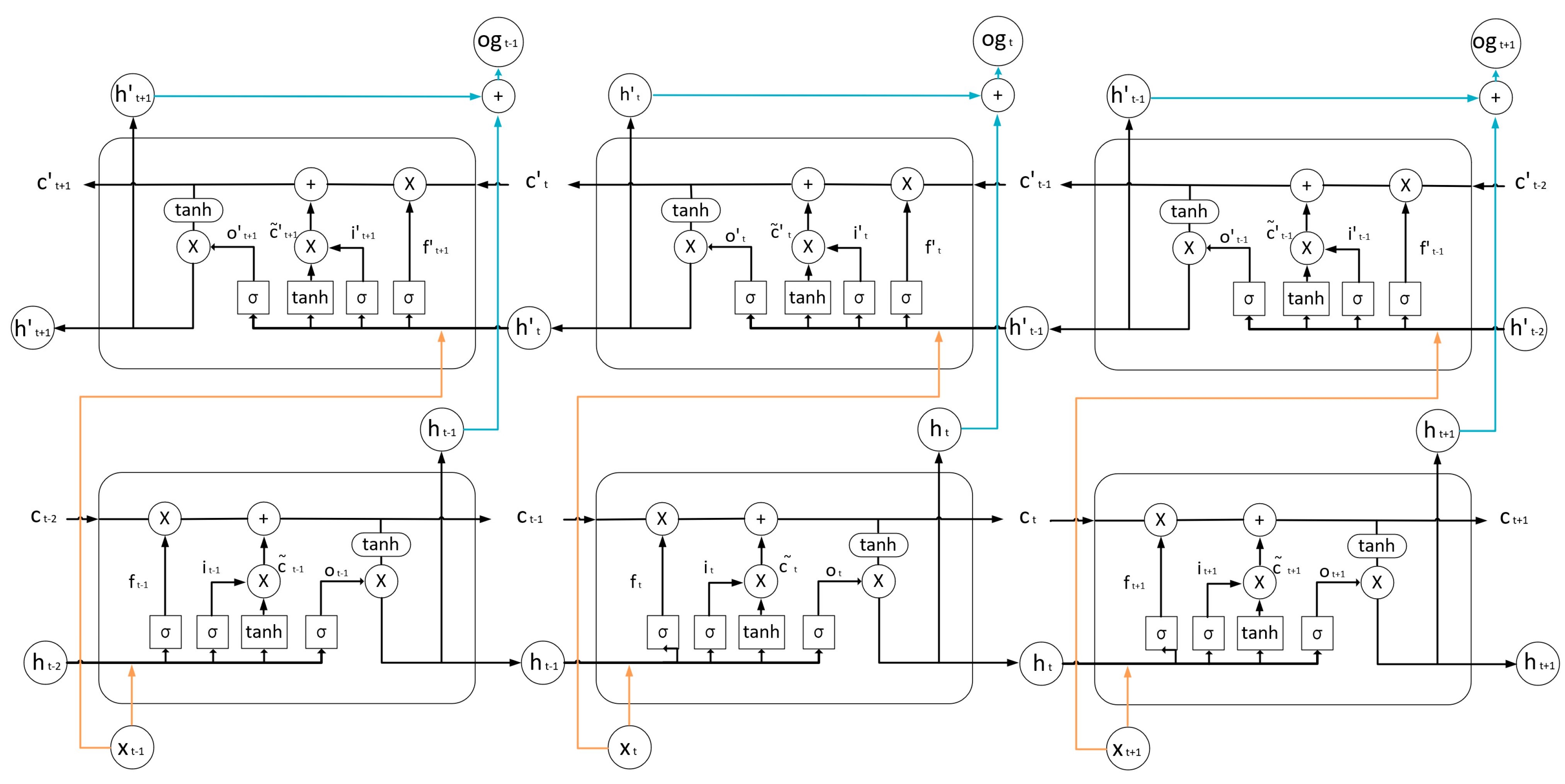
2.2.2. ConvBLSTM-PMwA Neural Network Model

Although LSTM has advantages in time series correlation calculations, the long-distance dependence of LSTM models still has the problem of gradient vanishing and gradient explosion. In this section, we introduce a CNN-based bi-directional LSTM parallel model with attention mechanism (ConvBLSTM-PMwA).

As shown in Figure 3, the input data are first extracted through a layer of CNN to extract the input features, which is called dense layer. A dropout layer is set, which will randomly drop part of the data. The dropout ratio is $dp$. In the next layer, a bi-LSTM network with opposite connections is used to process the information after dropout. The number of bi-LSTM blocks is a super-parameter that can be manually defined. The attention mechanism then merges important features together by changing the weight of the previous outcome. At last, the predicted result matrix has been generated, which includes the probability of different faults in the targeted future time span.

In the dense layer, CNNs are used for segment and feature extraction. The dimension of the dense layer can be expanded to fit the channels of the input data. This can deal with multiple sets of parallel data inputs, improving the scalability of the model. In this paper, our data sources are already combined into one channel, so the one-dimensional CNN layer is dense.

Figure 4 shows the Bi-LSTM network structure. We can see that the network learns intrinsic characteristics from past data and future data through a two-layer reverse chain structure and time series data.

In the attention layer, the weights of representations will be redistributed. The value of attention can be computed as below:

$${\mu }_t=\tanh \left(w_d\times flatten\left(o{g}_t^{\prime }s\right)+b_d\right)$$

(10)

$${\alpha }_t={\displaystyle \frac{\exp \left({\mu }_t{\mu }_d\right)}{{\sum }_t\mathrm{e}\mathrm{x}\mathrm{p} ({\mu }_t{\mu }_d)}},$$

(11)

where ${\mu }_t$ means the representation information of hidden layer, ${\mu }_d$ is the similarity of feature vectors, and ${\alpha }_t$ is the normalized weight.

The dense layer after attention layer is used to reduce the dimensionality of features to produce required prediction results. In this paper, as we need to predict FLC and LAC time series results at the same time, this layer has 2 channels.

2.3. Input Data for Online Calculation

Faults in a PEMFC are difficult to predict based on current state using model-based methods. The trained model detects if flooding and air starvation faults occur after a certain time based on the data we have at present time.

The input vectors are as follows:

$$X=\left[{\left[-T_{FC}-\right]}^T,{\left[-T_{airin}-\right]}^T,{\left[-P_{airin}-\right]}^T,{\left[-R{H}_{airin}-\right]}^T,{\left[-T_{airout}-\right]}^T,{\left[-P_{airout}-\right]}^T,{\left[-R{H}_{airout}-\right]}^T,{\left[-V-\right]}^T,{\left[-I-\right]}^T\right].$$

(12)

Among them, $T_{FC}$ is the infrared temperature of the fuel cell, $T_{air}$, $P_{air}$, and $R{H}_{air}$ represent the temperature, pressure, and relative humidity of the air inlet and outlet, respectively, $V$ is the output voltage of the fuel cell, and $I$ is the output current of the fuel cell. The superscript T in the upper corner indicates transpose, meaning that the input vectors are all column-vectors.

Figure 5 shows an example of input vector updating over time during online prediction. In this study, the $∆t$ is set to 1 s and the input time series is 60 s. The long red arrow indicates the time axis, and the green part represents the input vector, which is the collection of all data matrices collected by the sensor over time. The red parentheses indicate the duration of a set of input datasets, which is set at 60 seconds in this study. The blue parentheses indicate the datasets used for neural network prediction training. The target prediction duration will be adjusted during the specific training process. The ellipsis in the middle of the parentheses and to the right of the input vector indicates that the omitted part continues according to the rule described earlier.

2.4. Hyperparameter Selection and Tuning

2.4.1. LSTM Model Hyperparameter Tuning

The hyperparameters, number of LSTM layers, and nodes of each layer were tuned to improve the model’s efficiency. In the neural network structure, 9 models were created. The hyperparameters of the neural network models are listed in

Table 1. List of LSTM models with different hyperparameters.

Model	No. of LSTM Layers	Nodes of Each Layer
1	1	16
2	1	32
3	1	64
4	2	16
5	2	32
6	2	64
7	3	16
8	3	32
9	3	64

.

2.4.2. ConvBLSTM-PMwA Model Hyperparameter Tuning

The hyperparameter, the number of neuron units, is tuned to determine the best model. As the number of units increases, the total number of parameters for the model also increases dramatically. The hyperparameters of the neural network models are listed in

Table 2. ConvBLSTM-PmwA models with different neuron units.

Model	No. of Neuron Units	No. of Parameters
1	16	23,587
2	32	52,675
3	64	129,283
4	128	356,227

.

2.5. Post Processing

In this section, we first define two parameters to compare the results of the model.

$$R_t=\left\{\begin{array}{c}0r_t<0.2\\ \\ 1r_t>0.2\end{array}\right.$$

(13)

$$ACC={\displaystyle \frac{{\sum }_{t-∆T}^t{(R}_t\wedge {FLC}_{t+\Delta T})}{\Delta T}}\times 100\mathrm{\%}$$

(14)

$$CV={\displaystyle \frac{\sigma }{\mu }}$$

(15)

$$SEN={\displaystyle \frac{t_{fault}-t_{trig}}{t_{dt}-t_{trig}}}$$

(16)

Here, $r_t$ represents the predicted probability of flooding or air starvation fault occurring at a specific moment t. While in normal working state $r_t$ is near 0. The exact time when $R_t$ changes from 0 to 1 is the detection time $t_{dt}$. $\Delta T$ is the target future time for prediction in the neural network model; here, we set it to 60 s in the calculation. $ACC$ stands for accuracy, which indicates the consistency between the results calculated by the neural network and the manually marked ${FLC}_t$ within a target time $\Delta T$ in the future. ${FLC}_t$ is equal to the artificially labeled $FLC$ at a specific moment $t$ in the test data, and so is the ${LAC}_t$. The output prediction moment is determined by the growth rate of $r_t$, and $\mu$ refers to how many seconds in advance we are informed that the ${FLC}_t$ or ${LAC}_t$ is about to start changing, which is the average of multiple sets of the prediction results. $\sigma$ is the standard deviation of prediction time in different sets of tests. $CV$, the coefficient of variation, represents the ratio of the standard deviation $\sigma$ to the mean $\mu$. $SEN$ indicates the sensitivity of the model to predict fault, and the higher the value, the sooner the model can detect that the system is about to fail. $t_{trig}$ represents the time we manually change the operating condition. $t_{fault}$ represents the time when ${FLC}_t$ or $LA{C}_t$ change from 0 to 1.

3. Experiment

The setup of the experiment is shown in Figure 6. It consists of a fuel supply system, an air intake and humidification system, an infrared temperature sensor mounted on the fuel cell, temperature, humidity, and pressure sensors for the fuel cell intake and exhaust port, and electronic loads for tracking voltage and current. In this experimental setup, we keep the environment temperature at 25 °C. To accelerate flooding fault occurrence, three humidifiers were installed at the fuel cell’s air inlet to increase input air humidity. During testing, the inlet air humidity was not actively controlled to reflect actual operating environments where ambient humidity naturally fluctuates. Humidity data were monitored and recorded using sensors to document real-time variations. We ensure the mutual exclusion of both faults by isolating control parameters (e.g., blocking purge valve only for flood faults and blocking air inlets only for starvation faults). The collected data are humidity of anode and cathode, cell voltage, cell temperature, and impedance modulus. As a fault predictor based on deep learning, the fuel cell experiment recorded the data for more than 80 h, in which 40% were normal working data, 30% were flooding, and 30% were air starvation.

Temperature, pressure, and humidity measurements at both the fuel cell inlet and outlet were obtained using BME280 sensors, while surface temperature monitoring on the fuel cell casing employed an MLX90640 infrared thermal imaging module. Sensors are manufactured by Waveshare Electronics in Shenzhen, China. All sensors operated at a 1 Hz sampling frequency to ensure synchronized data collection.

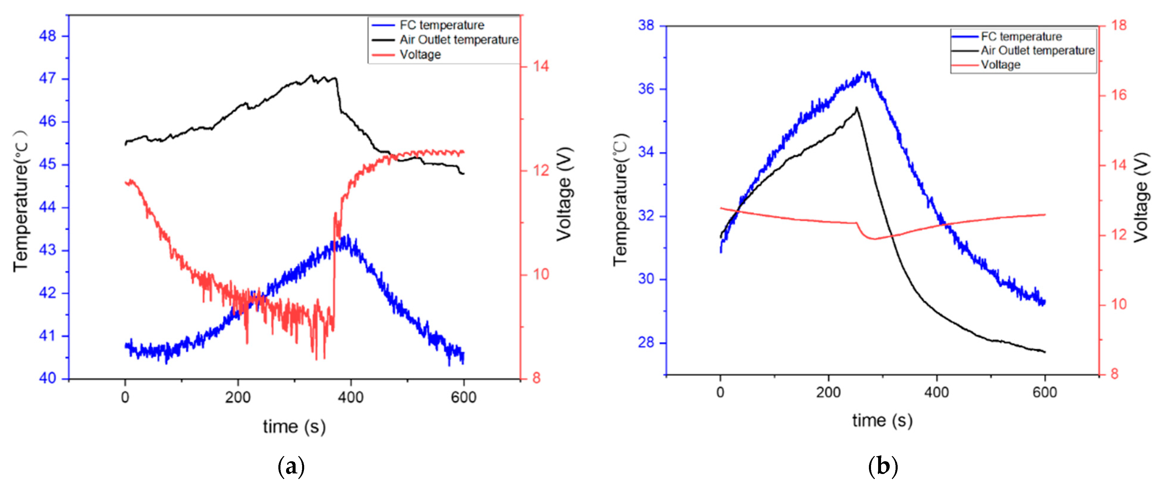
3.1. Flooding Experiment

The main process of the flooding fault data collection experiment is as follows. First, the fuel cell is stabilized under normal operating conditions for over one hour prior to experimental interventions. Set the purge valve to periodically purge it during this period to keep it in a relatively stable working condition without being too dry or risking flooding. It can be observed that part of the water is discharged from the fuel cell along with the purge process.

Subsequently, the manually controlled purge valve remains closed, thereby suspending fuel cell purge. After a period of time, the fuel cell is flooded and the output power subsequently drops. After recording the data for a period of time, the purge process is restarted. At this time, the water accumulated in the fuel cell will be discharged with the purge, and the output power of the fuel cell will start to rise. After waiting for the fuel cell output to return to a stable value in the normal state, repeat the above process and continuously record all sensor and electronic load data. During the experiment, set the electronic load working condition to keep the output current of the fuel cell constant.

3.2. Air Starvation Experiment

The main process of the air starvation fault data collection experiment is as follows. First, similar to the first step in Section 3.1, the fuel cell is stabilized under normal operating conditions for over one hour.

Subsequently, the fuel cell air inlet is manually blocked by a thin plastic sheet, thereby suspending the air supply to the fuel cell. After a period of time, the fuel cell falls into an oxygen-starved fault and the output power subsequently drops. After recording the data for a period of time, resume the air input. At this time, the fuel cell will gradually return to the normal working state, and the output power of the fuel cell will start to rise. After waiting for the fuel cell output to return to a stable value under normal conditions, repeat the above process to continuously record all sensor and electronic load data. During the experiment, set the electronic load to maintain a constant output current from the fuel cell.

4. Results and Discussion

4.1. Experiment Results

An example of the experimental data is shown in Figure 7. Here, Figure 7a shows the fuel cell voltage and temperature variation in the PEMFC during flooding fault and recovery and the temperature change at the air outlet during the above process. After the data recording started, the operator closed the hydrogen purge port of the fuel cell, which means that the water at the anode will gradually accumulate, manually creating a flood fault. As evidenced by the data, after the purge stops, the temperature of the fuel cell and the air outlet temperature exhibit a gradual increase because the purge of the anode also takes away the heat of the internal reaction of the fuel cell. Meanwhile, the decrease in the reaction power of the fuel cell is slower than the loss of heat dissipation efficiency. Since anode flooding prevents hydrogen from contacting the proton exchange membrane, the voltage of the fuel cell gradually decreases. Hydrogen purge functionality is reinstated after 370 s to facilitate fuel cell recovery from the flooding fault.

Figure 7b shows the fuel cell voltage and temperature variation in the PEMFC during air starvation fault and recovery and the temperature change at the air outlet during the above process. After the data logging started, the operator closed the fuel cell air intake, manually creating an air starvation fault. Since the air input does not only provide oxygen but is also the main way to cool the fuel cell, the fuel cell temperature and outlet temperature rise rapidly. Since the residual air inside the fuel cell can also participate in the reaction, the voltage drops slowly at first and, after a period of time, it begins to drop sharply. Air intake is restored after around 250 s to allow the fuel cell to recover from the air starvation fault.

4.2. Neural Network Results

4.2.1. LSTM Model Results

Using the data of the last 60 s, a prediction system for future PEMFC fault types and occurrence times is established. By comparing the prediction results under hyperparameters, the optimal model structure is selected. The difference in prediction performance under different neural network model hyperparameters is compared. The core software and hardware of deep learning equipment are Intel I9 12900K CPU, NVIDIA GeForce RTX 3080Ti GPU, 32 GB RAM.

From

Table 3. Results of LSTM models.

Model	Overall Accuracy (%)	Prediction Time (s)	CV (%)
1	96.03	59.43	36.01
2	95.61	35.31	75.84
3	96.15	31.58	112.45
4	97.94	42.32	39.54
5	95.99	27.41	84.48
6	95.90	59.65	17.07
7	95.06	4.39	86.26
8	96.67	26.10	72.18
9	96.18	37.28	83.60

and Figure 8a, it can be seen that Model 4 has the best accuracy and Model 6 has the longest prediction time, 59.65 s, and the smallest standard error (SE) with the smallest CV. From Figure 8b, it can be seen that Model 6 has the best sensitivity. Thus, the model with the best comprehensive effect is Model 6.

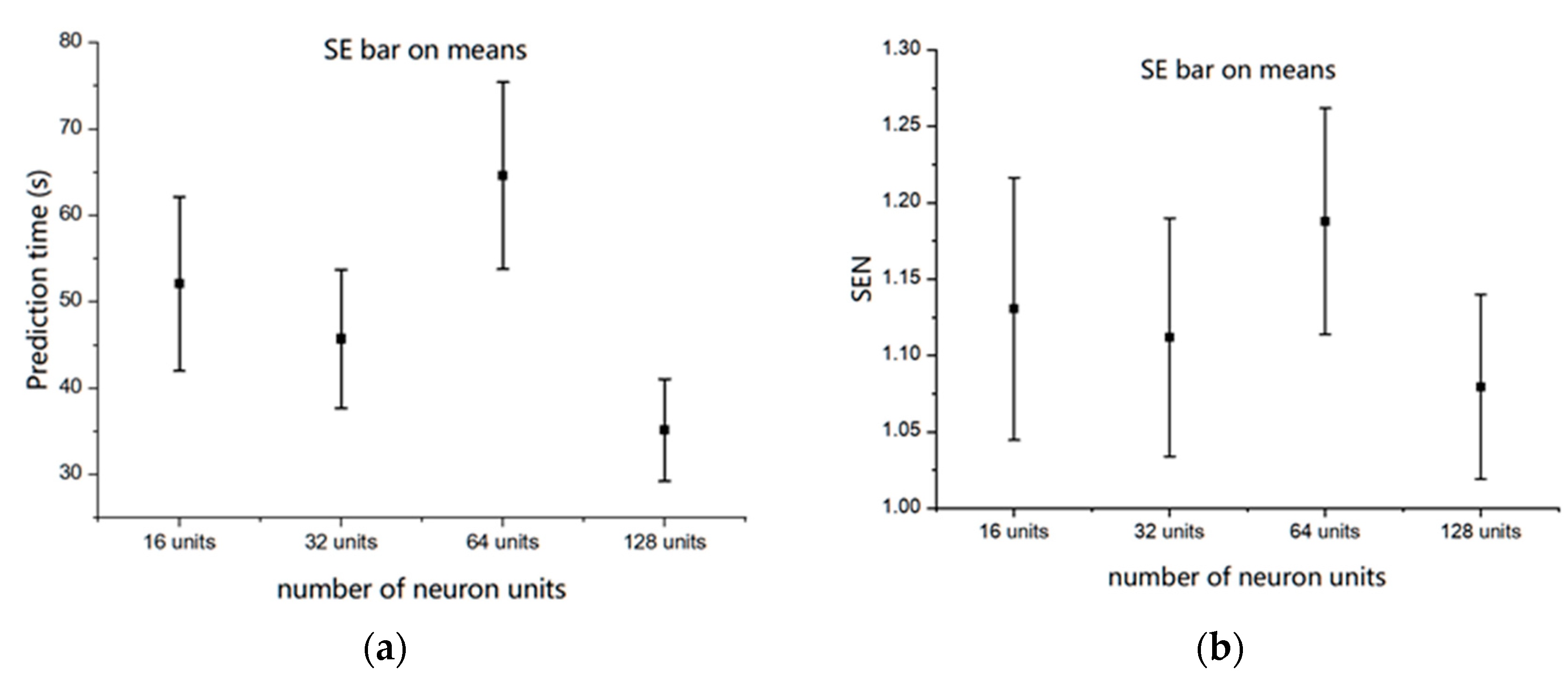
4.2.2. ConvBLSTM-PMwA Model Results

As shown in Figure 9, the accuracy has the best performance with a 0.3 dropout rate. The dropout rate has a negligible impact on the convergence results of loss. Therefore, we used 0.3 as the dropout rate in the ConvBLSTM-PMwA model and, subsequently, investigated the effect of changes in the structure of other model parameters.

Based on the results shown in

Table 4. Results of neural network models.

Model	Overall Accuracy (%)	Prediction Time (s)	CV (%)
16 units	95.91	52.08	19.36
32 units	97.28	45.72	17.52
64 units	96.49	64.63	16.73
128 units	94.68	35.16	16.82

and Figure 10a, the best number of neuron units is 64. It has the longest prediction time, the smallest CV, and the overall accuracy is relatively good. From Figure 10b, it can be seen that it also has the best sensitivity.

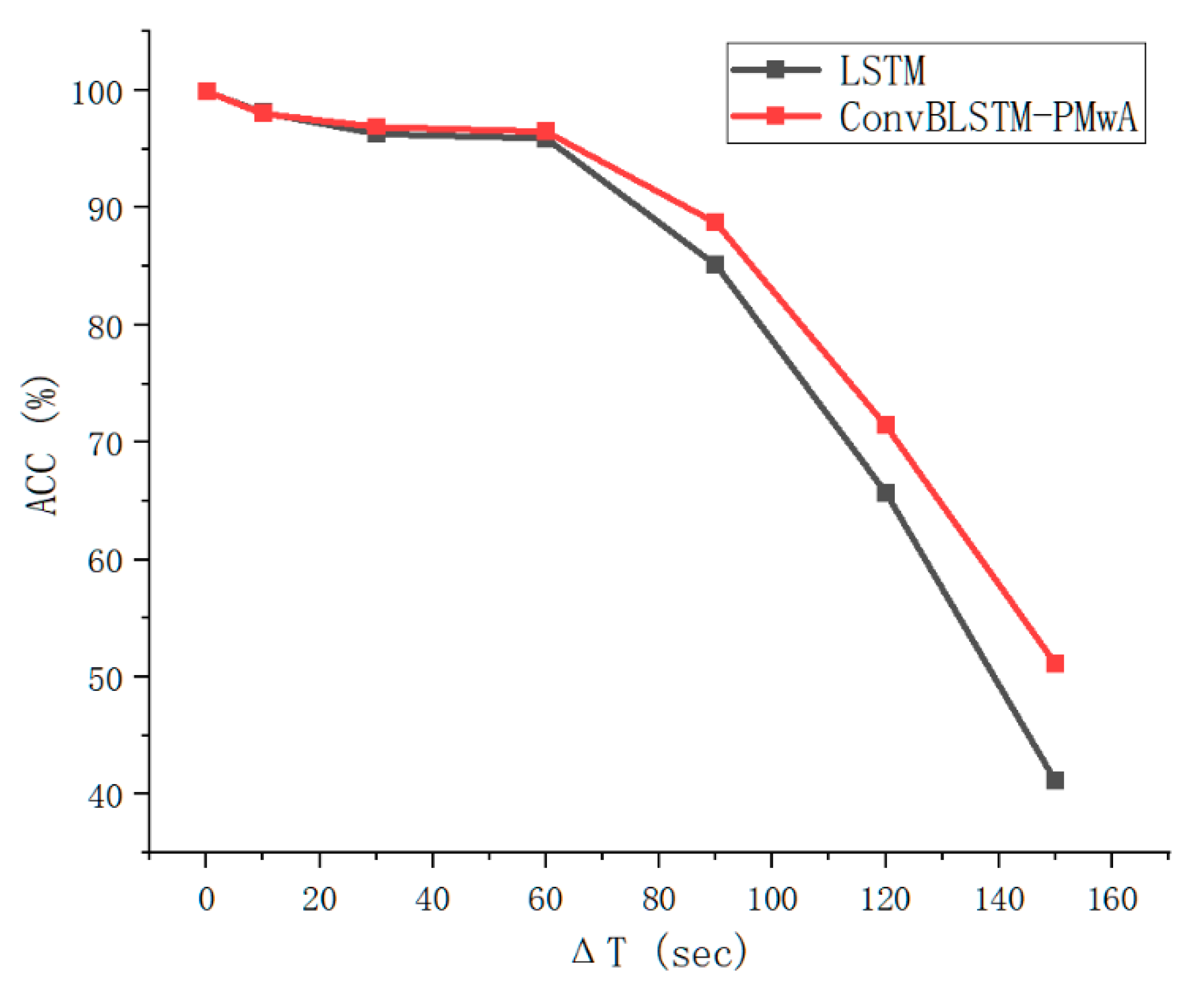
4.3. Performance of Different Prediction Times

The neural network method proposed in this paper can diagnose the type of fault and the time of fault occurrence that may occur after a period of time in the target PEMFC. This section discusses the relationship between the length of time the proposed model predicts future faults and the accuracy of the prediction. Here, we select both models in LSTM and ConvBLSTM-PMwA with the best prediction effect for this study.

Figure 11 shows the relationship between the prediction target time and the model’s prediction accuracy. Both models with a target time of 0 s can diagnose the fault of PEMFC almost accurately, but this is not a prediction and does not help prevent PEMFC faults. The accuracy from 10 s to 60 s decreases slightly, but the overall accuracy is still very high. However, the accuracy drops dramatically after 60 s and is almost unavailable at the target time of 150 s. It can be seen that the overall accuracy of the ConvBLSTM-PMwA model is higher than that of the LSTM model. When we need to predict faults for longer periods of time in advance, for example, 90 s, the ConvBLSTM-PMwA model has an 88.70% accuracy, which works better than the 85.11% accuracy in LSTM.

4.4. Performance of Prediction on Different Faults

Figure 12 shows the confusion matrix of the ConvBLSTM-PMwA model for two different faults (flooding and air starvation) when we set the prediction time to 60 s in the future. Each count represents a prediction made by the neural network for the next 60 s based on the data before this moment. The predictions of the neural network are calculated every second. It can be seen that the accuracy of flooding fault is 97.02%, the accuracy of air starvation fault is 94.21%, and the accuracy is 100% under normal working condition. It can be stated that the accuracies of the ConvBLSTM-PMwA model in predicting different types of fuel cell faults are sufficient for future adjustment procedures.

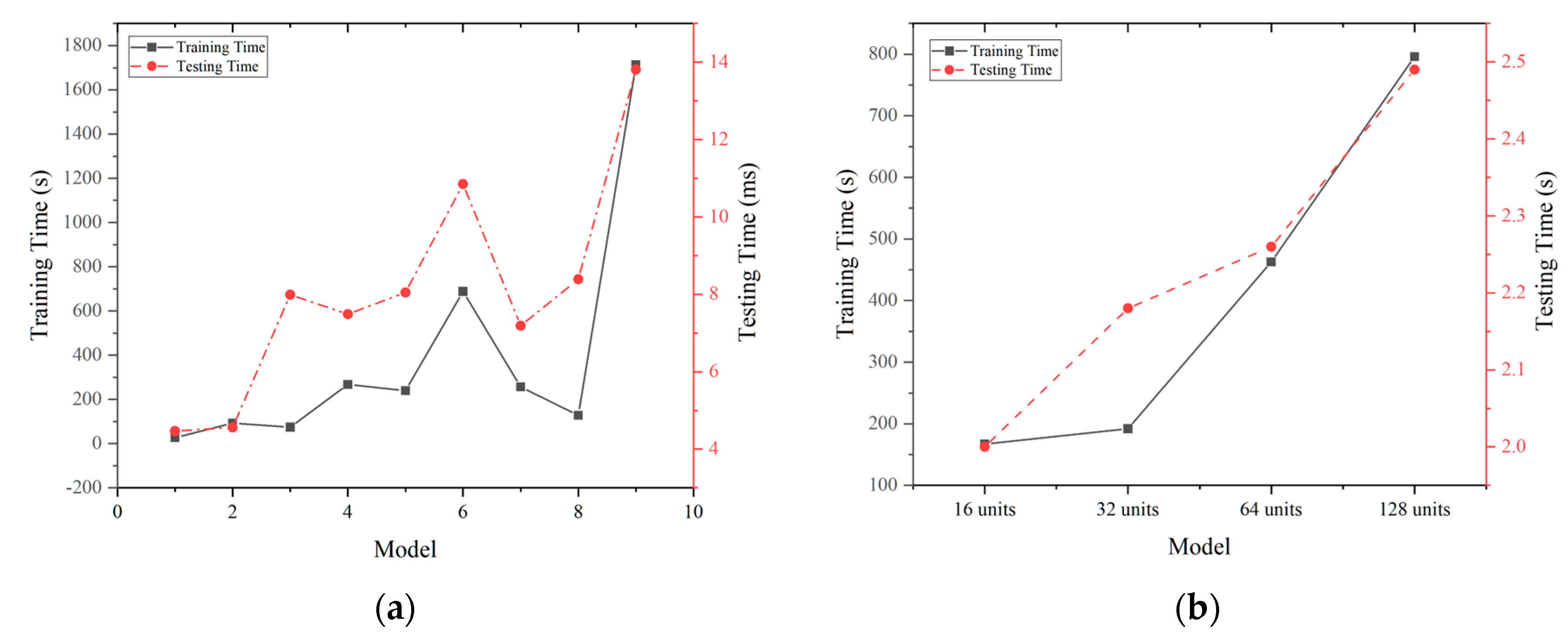
4.5. Training and Testing Time

Fault prediction models require not only excellent predictive performance but, also, fast enough computation. In this study, the training and testing times of different models are shown in Figure 13a,b. The training time is less important for this study because the training process is carried out in advance and does not affect the online prediction effect. Our main concern is the time it takes to obtain a predicted result in the test. From Figure 13a, we can see that Model 1 has the fastest prediction calculation, about 4.47 ms, and the maximum calculation time in the LSTM models is 13.81 ms. From Figure 13b, we can see that the training time increases as the number of units increases. In the case of more units, ConvBLSTM-PMwA’s training time will be significantly shorter than that of 3-layer LSTM models (such as Model 6 and Model 9). ConvBLSTM-PMwA has significantly more overall parameters than LSTM due to the more complex model structure, so its test time is significantly longer than that of the LSTM network. Since the control response and the state change in the fuel cell are not instantaneous, the calculation time of about 2 s is also acceptable in the online fault prediction and the control of the fuel cell system.

5. Conclusions

This study shows that we can infer future states using only sequential data up to the present of PEMFC, and the neural network is accurate in predicting flooding and air starvation faults that will occur in the near future. In this study, by tuning the structure and hyperparameters of the neural network model, a system was constructed to predict the flooding and air starvation faults of PEMFC.

The key findings of this study are summarized as follows:

• The best model for fault prediction in PEMFC systems is the 64-unit ConvBLSTM−PMwA model, which achieves an accuracy of 96.49% and a prediction time of 64.63 s before the fault occurs.
• The optimal prediction target time is 60 s, as shorter times reduce the repair time and longer times decrease prediction accuracy.
• The ConvBLSTM-PMwA model outperforms the LSTM model in long-term prediction accuracy, as it can extract more hidden features from the sensor data.

This study directly enhances fuel cell system reliability, reduces maintenance costs, and prolongs operational lifespan in practical applications like electric vehicles or distributed power systems. Future work will focus on extending the framework to diagnose additional fault types (e.g., membrane drying, hydrogen leakage) and integrating it with PEMFC control systems for closed-loop fault recovery under real-world dynamic conditions.

References

1. Zhao, Y.; Setzler, B.P.; Wang, J.; Nash, J.; Wang, T.; Xu, B.; Yan, Y. An Efficient Direct Ammonia Fuel Cell for Affordable Carbon-Neutral Transportation. Joule 2019, 3, 2472–2484. [Google Scholar] [CrossRef]
2. 2019 Fuel Cell Technologies Market Report. U.S. Department of Energy. Available online: https://publications.anl.gov/anlpubs/2021/08/166534.pdf (accessed on 6 June 2022).
3. Wang, Y.; Pang, Y.; Xu, H.; Martinez, A.; Chen, K.S. PEM Fuel cell and electrolysis cell technologies and hydrogen infrastructure development—A review. Energy Environ. Sci. 2022, 15, 2288–2328. [Google Scholar] [CrossRef]
4. Chen, H.; Zhao, X.; Zhang, T.; Pei, P. The reactant starvation of the proton exchange membrane fuel cells for vehicular applications: A review. Energy Convers. Manag. 2019, 182, 282–298. [Google Scholar] [CrossRef]
5. Huo, W.; Li, W.; Zhang, Z.; Sun, C.; Zhou, F.; Gong, G. Performance prediction of proton-exchange membrane fuel cell based on convolutional neural network and random forest feature selection. Energy Convers. Manag. 2021, 243, 114367. [Google Scholar] [CrossRef]
6. Wang, J. System integration, durability and reliability of fuel cells: Challenges and solutions. Appl. Energy 2017, 189, 460–479. [Google Scholar] [CrossRef]
7. Gu, X.; Hou, Z.; Cai, J. Data-based flooding fault diagnosis of proton exchange membrane fuel cell systems using LSTM networks. Energy AI 2021, 4, 100056. [Google Scholar] [CrossRef]
8. Kim, S.-G.; Lee, S.-J. A review on experimental evaluation of water management in a polymer electrolyte fuel cell using X-ray imaging technique. J. Power Sources 2013, 230, 101–108. [Google Scholar] [CrossRef]
9. Bodner, M.; Schenk, A.; Salaberger, D.; Rami, M.; Hochenauer, C.; Hacker, V. Air Starvation Induced Degradation in Polymer Electrolyte Fuel Cells. Fuel Cells 2017, 17, 18–26. [Google Scholar] [CrossRef]
10. Laribi, S.; Mammar, K.; Sahli, Y.; Koussa, K. Analysis and diagnosis of PEM fuel cell failure modes (flooding & drying) across the physical parameters of electrochemical impedance model: Using neural networks method. Sustain. Energy Technol. Assess. 2019, 34, 35–42. [Google Scholar]
11. Jiao, K.; Li, X. Water transport in polymer electrolyte membrane fuel cells. Prog. Energy Combust. Sci. 2011, 37, 221–291. [Google Scholar] [CrossRef]
12. Pang, Y.; Wang, Y. Water spatial distribution in polymer electrolyte membrane fuel cell: Convolutional neural network analysis of neutron radiography. Energy AI 2023, 14, 100265. [Google Scholar] [CrossRef]
13. Chen, H.; Zhang, Z.; Guan, C.; Gao, H. Optimization of sizing and frequency control in battery/supercapacitor hybrid energy storage system for fuel cell ship. Energy 2020, 197, 117285. [Google Scholar] [CrossRef]
14. Xu, J.-H.; Yan, H.-Z.; Zhang, B.-X.; Ding, Q.; Zhu, K.-Q.; Yang, Y.-R.; Wan, Z.-M.; Lee, D.-J.; Wang, X.-D.; Tu, Z.-K. Multi-criteria evaluation and optimization of PEM fuel cell degradation system. Appl. Therm. Eng. 2023, 227, 120389. [Google Scholar] [CrossRef]
15. Dhimish, M.; Vieira, R.G.; Badran, G. Investigating the stability and degradation of hydrogen PEM fuel cell. Int. J. Hydrogen Energy 2021, 46, 37017–37028. [Google Scholar] [CrossRef]
16. Yang, Y.; Gao, Y.; Liu, Z.; Zhang, X.; Meng, F.; Wang, J.; Zhang, J.; Zhao, P.; Li, P.; He, X. Simultaneous measurement of local current and temperature distributions in proton exchange membrane fuel cells with dead-ended anode. Appl. Therm. Eng. 2023, 230, 120728. [Google Scholar] [CrossRef]
17. Rahimi-Esbo, M.; Ramiar, A.; Ranjbar, A.A.; Alizadeh, E. Design, manufacturing, assembling and testing of a transparent PEM fuel cell for investigation of water management and contact resistance at dead-end mode. Int. J. Hydrogen Energy 2017, 42, 11673–11688. [Google Scholar] [CrossRef]
18. Banerjee, R.; Ge, N.; Han, C.; Lee, J.; George, M.G.; Liu, H.; Muirhead, D.; Shrestha, P.; Bazylak, A. Identifying in operando changes in membrane hydration in polymer electrolyte membrane fuel cells using synchrotron X-ray radiography. Int. J. Hydrogen Energy 2018, 43, 9757–9769. [Google Scholar] [CrossRef]
19. Sinha, P.K.; Halleck, P.; Wang, C.-Y. Quantification of Liquid Water Saturation in a PEM Fuel Cell Diffusion Medium Using X-ray Microtomography. Electrochem. Solid-State Lett. 2006, 9, A344. [Google Scholar] [CrossRef]
20. Iranzo, A.; Gregorio, J.M.; Boillat, P.; Rosa, F. Bipolar plate research using Computational Fluid Dynamics and neutron radiography for proton exchange membrane fuel cells. Int. J. Hydrogen Energy 2020, 45, 12432–12442. [Google Scholar] [CrossRef]
21. Mishler, J.; Wang, Y.; Mukundan, R.; Spendelow, J.; Hussey, D.S.; Jacobson, D.L.; Borup, R.L. Probing the water content in polymer electrolyte fuel cells using neutron radiography. Electrochim. Acta 2012, 75, 1–10. [Google Scholar] [CrossRef]
22. Damour, C.; Benne, M.; Grondin-Perez, B.; Bessafi, M.; Hissel, D.; Chabriat, J.-P. Polymer electrolyte membrane fuel cell fault diagnosis based on empirical mode decomposition. J. Power Sources 2015, 299, 596–603. [Google Scholar] [CrossRef]
23. Debenjak, A.; Gašperin, M.; Pregelj, B.; Atanasijević-Kunc, M.; Petrovčič, J.; Jovan, V. Detection of flooding and drying inside a PEM fuel cell stack. J. Mech. Eng. 2013, 59, 56–64. [Google Scholar] [CrossRef]
24. Ren, P.; Pei, P.; Li, Y.; Wu, Z.; Chen, D.; Huang, S.; Jia, X. Diagnosis of water failures in proton exchange membrane fuel cell with zero-phase ohmic resistance and fixed-low-frequency impedance. Appl. Energy 2019, 239, 785–792. [Google Scholar] [CrossRef]
25. Mammar, K.; Saadaoui, F.; Laribi, S. Design of a PEM fuel cell model for flooding and drying diagnosis using fuzzy logic clustering. Renew. Energy Focus 2019, 30, 123–130. [Google Scholar] [CrossRef]
26. Chen, X.; Xu, J.; Fang, Y.; Li, W.; Ding, Y.; Wan, Z.; Wang, X.; Tu, Z. Temperature and humidity management of PEM fuel cell power system using multi-input and multi-output fuzzy method. Appl. Therm. Eng. 2022, 203, 117865. [Google Scholar] [CrossRef]
27. Pan, T.; Shen, J.; Sun, L.; Lee, K.Y. Thermodynamic modelling and intelligent control of fuel cell anode purge. Appl. Therm. Eng. 2019, 154, 196–207. [Google Scholar] [CrossRef]
28. Chen, K.; Laghrouche, S.; Djerdir, A. Aging prognosis model of proton exchange membrane fuel cell in different operating conditions. Int. J. Hydrogen Energy 2020, 45, 11761–11772. [Google Scholar] [CrossRef]
29. Yuan, H.-B.; Zou, W.-J.; Jung, S.; Kim, Y.-B. Optimized rule-based energy management for a polymer electrolyte membrane fuel cell/battery hybrid power system using a genetic algorithm. Int. J. Hydrogen Energy 2022, 47, 7932–7948. [Google Scholar] [CrossRef]
30. Ma, T.; Zhang, Z.; Lin, W.; Yang, Y.; Yao, N. A Review on Water Fault Diagnosis of a Proton Exchange Membrane Fuel Cell System. J. Electrochem. Energy Convers. Storage 2021, 18, 030801. [Google Scholar] [CrossRef]
31. Yousfi Steiner, N.; Hissel, D.; Moçotéguy, P.; Candusso, D. Diagnosis of polymer electrolyte fuel cells failure modes (flooding & drying out) by neural networks modeling. Int. J. Hydrogen Energy 2011, 36, 3067–3075. [Google Scholar]
32. Zuo, B.; Zhang, Z.; Cheng, J.; Huo, W.; Zhong, Z.; Wang, M. Data-driven flooding fault diagnosis method for proton-exchange membrane fuel cells using deep learning technologies. Energy Convers. Manag. 2022, 251, 115004. [Google Scholar] [CrossRef]
33. Yu, X.; Pingwen, M.; Ming, H.; Baolian, Y.; Shao, Z.-G. The critical pressure drop for the purge process in the anode of a fuel cell. J. Power Sources 2009, 188, 163–169. [Google Scholar] [CrossRef]
34. Mao, L.; Jackson, L.; Davies, B. Investigation of PEMFC fault diagnosis with consideration of sensor reliability. Int. J. Hydrogen Energy 2018, 43, 16941–16948. [Google Scholar] [CrossRef]
35. Kim, K.; Kim, J.; Choi, H.; Kwon, O.; Jang, Y.; Ryu, S.; Lee, H.; Shim, K.; Park, T.; Cha, S.W. Pre-diagnosis of flooding and drying in proton exchange membrane fuel cells by bagging ensemble deep learning models using long short-term memory and convolutional neural networks. Energy 2023, 266, 126441. [Google Scholar] [CrossRef]
36. Yin, X.; Liu, Z.; Liu, D.; Ren, X. A Novel CNN-based Bi-LSTM parallel model with attention mechanism for human activity recognition with noisy data. Sci. Rep. 2022, 12, 7878. [Google Scholar] [CrossRef]
Figure 1. Block diagram of the workflow.
Energies 18 02669 g001
Figure 2. Architecture of our LSTM model.
Energies 18 02669 g002
Figure 3. Block diagram of the ConvBLSTM−PMwA neural network model.
Energies 18 02669 g003
Figure 4. Bi−LSTM network with three blocks.
Energies 18 02669 g004
Figure 5. Sliding update input vector for online prediction.
Energies 18 02669 g005
Figure 6. Experimental setup for PEMFC.
Energies 18 02669 g006
Figure 7. (a) An example of PEMFC experiment data during flooding and recovery (temperature: 25 ± 1°C, RH: 60 ± 5%). (b) An example of PEMFC experiment data during air starvation and recovery (temperature: 25 ± 1 °C, RH: 60 ± 5%).
Energies 18 02669 g007
Figure 8. (a) Prediction time of LSTM models. (b) Sensitivity of LSTM models.
Energies 18 02669 g008
Figure 9. The loss and accuracy with different dropout rates.
Energies 18 02669 g009
Figure 10. (a). Prediction time of ConvBLSTM-PMwA. (b) Sensitivity of ConvBLSTM-PMwA.
Energies 18 02669 g010
Figure 11. The accuracy with different target future time for prediction.
Energies 18 02669 g011
Figure 12. The confusion matrix of different faults at the target prediction time of 60 s.
Energies 18 02669 g012
Figure 13. (a) Time used by LSTM models. (b) Time used by ConvBLSTM−PMwA models.
Energies 18 02669 g013