A Techno-Economic Analysis of Power Generation in Wind Power Plants Through Deep Learning: A Case Study of Türkiye

Abstract

In recent years, the utilization of renewable energy sources has significantly increased due to their environmentally friendly nature and sustainability. Among these sources, wind energy plays a critical role, and accurately forecasting wind power with minimal error is essential for optimizing the efficiency and profitability of wind power plants. This study analyzes hourly wind speed data from 23 meteorological stations located in Türkiye’s Western Black Sea Region for the years 2020–2024, using the Weibull distribution to estimate annual energy production. Additionally, the same data were forecasted using the Long Short-Term Memory (LSTM) model. The predicted data were also assessed through Weibull distribution analysis to evaluate the energy potential of each station. A comparative analysis was then conducted between the Weibull distribution results of the measured and forecast datasets. Based on the annual energy production estimates derived from both datasets, the revenues, costs, and profits of 10 MW wind farms at each location were examined. The findings indicate that the highest revenues and unit electricity profits were observed at the Zonguldak South, Sinop İnceburun, and Bartın South stations. According to the LSTM-based forecasts for 2025, investment in wind energy projects is considered feasible at the Sinop İnceburun, Bartın South, Zonguldak South, İnebolu, Cide North, Gebze Köşkburnu, and Amasra stations.

1. Introduction

The energy industry has gained strategic importance since the 1970s. Energy security, the sustainability of the energy supply, and its transfer to future generations are of strategic significance. The rapid depletion of carbon-based fossil fuels, along with their significant contribution to environmental pollution, has made the adoption of alternative, environmentally friendly, and renewable energy sources inevitable. As a result, greater emphasis is being placed on renewable energy to meet the growing global energy demand. In fact, in certain countries, energy generated from renewable sources has already surpassed that produced from conventional energy systems [1].

In 2023, Türkiye’s total electricity generation reached 328.1 TWh, with renewable energy sources—excluding hydroelectric power—accounting for approximately 25% of this total. Notably, the share of wind energy experienced a record increase compared to the previous year, rising to 10.12% of the total electricity production [2]. Sustaining the momentum in wind energy investments largely depends on the effective assessment of regional wind energy potential. While various statistical methods have traditionally been employed to estimate wind potential, recent advancements have led to the widespread application of Long Short-Term Memory (LSTM) networks—originally developed for time series forecasting in fields such as speech recognition and machine translation—in the prediction of wind speeds [3]. Machine learning techniques enable more accurate forecasting in energy production planning, thereby contributing to improved decision-making and resource allocation [4]. In particular, the LSTM approach has been shown to yield successful results in long-term forecasting applications [5]. With the aim of achieving more accurate wind power forecasts using machine learning techniques, this study evaluates the wind energy investment potential across five provinces in Türkiye’s Western Black Sea Region. In this context, wind speed data are predicted using LSTM model, a widely used method in machine learning. The measured and predicted wind speed data are separately analyzed to estimate the parameters of the Weibull distribution. These parameters are then used to calculate the Weibull power density and the annual energy production. A comparison is made between the results derived from the measured datasets and those obtained through LSTM-based predictions. Additionally, an investment cost analysis is conducted based on annual energy output. The technical and economic aspects of wind energy are discussed in Section 2; the methodology is presented in Section 3; data analysis and our results are presented in Section 4; our interpretation of the findings is provided in Section 5; and the conclusions, limitations, and recommendations are outlined in Section 6.

2. Literature Review

2.1. Related Studies in Wind Power Plant Technical Potential Analysis

The increasing air pollution and the reckless use of fossil fuels worldwide have steadily heightened the interest of researchers and policymakers in renewable energy sources [6]. It is evident that investments in wind energy have gained significant momentum over time compared to other renewable energy sources [7]. In addition to the generation of electricity from wind energy, its sustainability is also of paramount importance. The variability of wind speed, meaning that it does not remain constant, presents a significant uncertainty when evaluating wind power plants. Therefore, for the optimization of wind energy investments, it is essential to realistically forecast wind speed and, consequently, wind energy [8]. In this context, the data and methods used for accurately forecasting wind power are of critical importance. Statistical approaches have traditionally been employed in wind speed forecasting, with machine learning methods, which have gained significant popularity in recent years, becoming increasingly preferred [9].

Machine learning, deep learning models, and artificial intelligence techniques have garnered significant attention from researchers due to their ability to uncover new insights and deliver exceptional performance in the analysis of nonlinear relationships. An increase in studies utilizing deep learning methods in solar and wind energy research can be observed in the Web of Science database. In many of these studies, the success achieved in wind power forecasting demonstrates the potential applicability of these methods [10]. Furthermore, [11] indicates that deep learning methods can be applied not only in wind energy forecasting but also in wave energy prediction. The potential of deep learning techniques in energy optimization, energy management, and electricity generation forecasting is highlighted. In a similar study on wind energy optimization, [12] emphasizes that accurately forecasting the temporal distribution of measured wind speed has a significant impact on energy production. In Austria, the optimization of wind energy has been achieved by combining Complete Ensemble Empirical Mode Decomposition with Adaptive Noise (CEEMDAN) and LSTM methods, resulting in wind power predictions with minimal error.

Machine learning methods such as Recurrent Neural Networks (RNNs), Long Short-Term Memory (LSTM), Gated Recurrent Units (GRUs), Bidirectional Long Short-Term Memory (BiLSTM), and techniques like Bagging and Extreme Gradient Boosting (XGBoost) are commonly employed in wind speed forecasting [13,14,15]. Forecasting can be performed using one or a combination of these methods.

In time series forecasting, wind energy is predicted using methods such as Functional Neural Networks (FNNs) and LSTM [16]. These methods have demonstrated successful results by providing stable and accurate power output predictions, and they have even been suggested for predicting the likelihood of turbine failure. In a similar study, [17] combines time series and Artificial Neural Networks (ANNs) in a hybrid method. It is noted that, depending on various criteria such as time, input features, computation time, and error metrics, this hybrid approach is one of the most suitable forecasting methods for wind power in wind turbines/farms.

It has been indicated that, among methods such as LSTM, Artificial Neural Networks (ANNs), Support Vector Machines (SVMs), Convolutional Neural Networks (CNNs), and Extreme-Learning Machines (ELMs), the LSTM method provides the best predictions [18]. In another study [19], it was stated that wind power forecasting with CNNs and LSTM methods yielded successful results. [20] emphasized in their study that CNNs and LSTM methods provided better results in detecting temporal dependencies and nonlinear relationships in wind power forecasting. Similarly, a study utilizing Correntropy LSTM for wind power prediction based on meteorological data achieved successful forecasts [21]. The use of hybrid methods in machine learning has led to successful outcomes. [10] mentioned that the combination of RNN, LSTM, and CNN methods in a hybrid model is preferred for probability calculations and forward forecasting. In another study [22], it was noted that wind speed, direction, generated power, and theoretical power were predicted using the LSTM method, aligned with real-life scenarios.

Hybrid models that integrate machine learning methods with probability distributions also exist. For instance, wind power can be forecasted by combining the Weibull distribution with Recurrent Neural Networks (RNNs). The RNN method is suitable for short-term wind power forecasting [13]. Ref. [14] noted that, for short-term wind power prediction, the Graph Network Model, Random Sampling Algorithm (RSA), and LSTM methods provide more accurate forecasts based on both time and spatial dimensions.

Multi-Criteria Decision-Making methods are also applied in wind energy forecasting. [23] examined the efficiency of floating wind farms in the Canary Islands using Multi-Criteria Decision-Making (MCDM) methods, emphasizing that four areas were suitable for establishing wind farms. It was even pointed out that the most optimal locations for the establishment of wind farms were those located 1000 m deep in the sea. The analysis’ findings suggest that MCDM methods could be used in wind energy plant investments.

In a recent study, Shayan et al. utilized Markov Chains—commonly employed in the analysis of dynamic and stochastic systems, such as wind speed, which vary over time—to address the uncertainty in wind power. Additionally, the Autoregressive Moving Average (ARMA) model was used to forecast the needs of a Microgrid (MG) [24]. In their study, Shayan et al. (2024) proposed a cost-minimizing power system for wind energy production by introducing a machine learning-based two-stage Adaptive Robust Optimization (ARO) system. This approach integrated Data-Driven Techniques (DDTs) and Disjunctive Data Uncertainty (DDU) to develop a robust optimization method [25].

The reviewed studies highlight that deep learning models, by utilizing real data, have provided successful results in wind power forecasting. The challenges related to the scattered nature of wind, fluctuations in wind power, and the difficulty in predicting wind speed and power underscore the success of deep learning methods [8]. In this study, the real data and the predictions made with the LSTM model are compared through the Weibull distribution, a statistical method. Additionally, investment costs are evaluated for both outcomes. The hybrid use of both methods is expected to contribute to the literature.

2.2. Related Studies in Wind Power Plant Investment and Economic Analysis

In the city of Deokjeok-do, South Korea, the potential for WPP investment was researched, and the unit cost of electricity was determined to be 0.077 EUR/kWh, the internal rate of return (IRR) of the investment was 8.13%, and the payback period was 9.72 years [26]. In a study conducted in Jordan, wind energy investment potential was examined at five different locations. The cost of the energy derived from wind power ranged between 0.0259 USD/kWh and 0.0498 USD/kWh at the best location, while at the worst location, it was found to be 0.222 USD/kWh. However, even this cost was still lower than those of conventional fuels [27]. In a study examining wind energy investment potential in two cities in Sindh province, Pakistan, it was stated that energy costs ranged between 0.056 USD/kWh and 0.074 USD/kWh [28]. In Hyderabad, Pakistan, it was determined that the unit cost of wind energy in wind power plants ranged from 19.27 USD/mWh to 32.80 USD/mWh [29]. A study conducted in Nigeria using data from a height of 10 m found that energy costs ranged between 4.02 NGN/kWh and 166.79 NGN/kWh for wind energy potential [30]. In Ghana, it was determined that the unit energy cost of a wind power plant was 0.143 USD/kWh, and since the price tariff was 0.15 USD/kWh, the investment was deemed irrational [31]. In Calgary, Canada, using 25 years of wind speed data, it was predicted that electricity could be produced at a unit cost of 0.09 CAD/kWh [1]. In a feasibility analysis conducted in different cities in Iran, the prices of electricity produced by small wind power plants ranged from 0.074 USD/kWh to 0.348 USD/kWh, while large plants produced electricity at prices ranging from 0.047 USD/kWh to 0.182 USD/kWh [32].

The findings of this study indicate that deep learning methods, particularly the LSTM model, have demonstrated higher accuracy in wind energy forecasting compared to traditional statistical approaches. Improved forecasting performance has contributed to more accurate estimations of electricity unit costs, further emphasizing the economic advantage of wind energy over conventional fossil fuels.

In this context, the LSTM deep learning approach was employed in this study to predict long-term wind power generation. To assess the effectiveness of the forecasting model, the results produced by the LSTM method were compared with those derived from the Weibull probability distribution—a commonly used statistical technique in wind energy analysis. Following the prediction of the wind power plants’ electricity generation potential, economic evaluations were conducted for both methodologies.

Based on the outcomes of this comparative analysis, recommendations were formulated for policymakers. These include guidance on assessing the economic performance of wind power plant investments, optimizing electricity generation planning, and supporting informed, cost-effective investment decision-making in the renewable energy sector.

3. Materials and Methods

In this study, wind speed data obtained from stations located in the Western Black Sea Region of Türkiye were analyzed. The wind speed data were obtained from the Meteorological General Directorate’s measurement stations at a height of 10 m [33]. The wind speed measurements conducted by the General Directorate of Meteorology were carried out within the scope of quality standards. These measurements were performed using anemometer devices. The calibration of these devices was carried out in accordance with the TS EN ISO/IEC 17025 quality standard of the Turkish Accreditation Agency (TÜRKAK) [34]. Similar studies in the literature have also utilized data measured at a height of 10 m [30]. When establishing a wind power plant, the wind speed at the installation height of the turbines is considered to determine the turbine power. This study planned to establish a wind farm consisting of 1 MW turbines produced by the Soyutwind company. The specifications of the 1 MW turbine are as follows: a rated wind speed of 12 m/s, cut-in wind speed of 4 m/s, cut-out wind speed of 25 m/s, rotor diameter of 70 m, swept area of 3848.5 m², and an average tower height of 65 m [35]. This study planned to establish a power plant consisting of 1 MW turbines. Therefore, wind turbine parameters with a tower height of 65 m were used. For this purpose, wind power could be calculated using Formula (1) [36]:

$$\left({\displaystyle \frac{v}{v_0}}\right)={\left({\displaystyle \frac{h}{h_0}}\right)}^{\alpha }$$

(1)

Here, v₀ refers to the reference wind speed, h₀ refers to the reference height, h is the height at which the wind speed is to be calculated, v is the wind speed at height h, and α is the friction coefficient. The friction coefficient, α, is a parameter that needs to be determined. The topographic structure of the Western Black Sea Region consists of a long coastline and extensive forested areas. For the coastal areas, the α value ranged from 0.10 to 0.15, while in forested areas, it varied between 0.25 and 0.30 [37]. The friction coefficient for the analyzed region could be selected within the range of 0.1 to 0.3. In this study, the α value was considered as 0.2 on average.

The study sample consisted of five coastal cities and 23 stations located in the Western Black Sea Region of Türkiye’s northern Black Sea area. A map illustrating the locations of all the stations is presented in Figure 1 [38]. This region was expected to experience higher wind speeds due to the prevailing wind patterns in the northern cities.

The hourly average wind speed data for the 23 stations from 2020 to 2024 were evaluated. Using wind data measured at a height of 10 m at each station, the data for a height of 65 m were calculated using Equation (1). The prediction of wind speed data at 65 m was performed using the two-parameter Weibull distribution. Additionally, using the 5-year wind speed data at 65 m for all locations, wind speed data for the following year were forecasted using LSTM networks. The predicted data were then evaluated using the Weibull distribution. Wind power for both the real and predicted data were determined, and cost analyses were compared.

3.1. Weibull Distribution

The Weibull distribution, developed by Waloddi Weibull in 1951, is a highly useful and widely used method for the analysis of wind speed data [39]. The two-parameter Weibull probability density function (PDF) and cumulative distribution function (CDF) can be expressed as follows [39,40]:

$$f_w(v)={\displaystyle \frac{k}{\lambda }}{\left({\displaystyle \frac{v}{\lambda }}\right)}^{k-1}\exp \left[-{\left({\displaystyle \frac{v}{\lambda }}\right)}^k\right]$$

(2)

$$F_w(v)={\displaystyle \underset{0}{\overset{v}{\int }}{f}_w(v)=1-}\exp \left[-{\left({\displaystyle \frac{v}{\lambda }}\right)}^k\right]$$

(3)

Here, λ represents the scale parameter, k represents the shape parameter, and v represents the wind speed. In Equation (2), the wind speed (v) must take a value greater than zero (v > 0). The shape parameter is an important factor in assessing the nature of the wind speed distribution. Small values of the shape parameter indicate greater fluctuations around the average wind speed, while larger values suggest smaller fluctuations around the mean wind speed [41]. There are several methods for determining the parameters of the Weibull distribution. In this study, the Maximum Likelihood Estimation (MLE) method was employed to determine the parameters of the probability distribution. MLE is a widely used statistical technique for estimating the parameters of a given probability distribution. The method is fundamentally based on maximizing the likelihood function, which represents the probability of observing the given data under specific parameter values. The parameter estimates obtained through this method correspond to the values that maximize the likelihood function, and are therefore considered the most probable [42]. For the Weibull distribution, the parameters k and λ can be calculated using the maximum likelihood method, as shown in the respective equations [43].

$$k={\left({\displaystyle \frac{{\displaystyle \sum _{i=1}^n{v}_i^k\ln (v_i)}}{{\displaystyle \sum _{i=1}^n{v}_i^k}}}-{\displaystyle \frac{{\displaystyle \sum _{i=1}^n\ln (v_i)}}{n}}\right)}^{-1}$$

(4)

$$\lambda ={\left({\displaystyle \frac{{\displaystyle \sum _{i=1}^n{\left(v_i\right)}^k}}{n}}\right)}^{{\displaystyle \frac{1}{k}}}$$

(5)

Here, n represents the total number of wind speed data points in the dataset, and v_i represents the hourly wind speed data in the dataset.

3.2. Long Short-Term Memory (LSTM)

LSTM is a specialized type of Recurrent Neural Network (RNN), which consists of fundamental layers such as input, hidden, and output layers. Like RNNs, LSTM also has recurrent connections. Due to their ability to learn long-term dependencies between data points in a dataset, LSTM models are highly useful in processing sequential data and making predictions based on those data. LSTM models offer a significant solution to the vanishing gradient problem and feature forget gates that control which information from the hidden state will be passed to the next hidden state as an output [4,16,44,45]. For these reasons, LSTM models are widely used in time series forecasting, such as with hourly wind speed data over one or more years. The LSTM neural network structure is shown in Figure 2. Due to their capabilities, LSTM networks are commonly used for time series prediction, such as of hourly wind data over one or more years. The structure of the LSTM neural network is presented in Figure 2, and the fundamental components and operations of LSTM are as follows:

• Input gate: The input gate allows for the storage of new prediction data in the cell state, which carries data like a communication line within the cells. This layer contains both sigmoid and tanh functions. The sigmoid function is used to decide which data will be updated, while the tanh function is used to generate new data when needed [4,47,48].
• Output gate: The output gate regulates the flow of information from the memory cell to the hidden state. Similarly to the input gate, it contains a sigmoid and tanh function for the determination of the hidden state and prediction [4,16].
• Forget gate: The forget gate evaluates which data should be forgotten and which should be retained from the cell state. A sigmoid activation function, which produces values between 0 and 1, is used to determine how much of the past data should be retained or forgotten. If the function output is 0, the data are forgotten, and if the output is 1, the data are retained and continues to be carried along with the cell state [4,49].

In this study, hourly wind data from 23 stations for the years 2020–2024 were used to predict hourly wind speeds for the years 2021–2025 using an LSTM model. The forecasting for each station was conducted independently with the measured data from the years 2020, 2021, 2022, 2023, and 2024. As an example, for the Akçakoca Fener station, five predictions were made, one for each year between 2020 and 2024. In total, 115 independent analyses were carried out. Initially, outliers, such as zero values, were removed from the wind dataset, and missing data were filled in with mean values. The model input, x(t) = [WindSpeed(t)], and output, y(t) = [WindSpeed(t)], consisted of a single variable, representing one-hour wind data. For the LSTM model, 80% of the wind speed data were used for training, and 20% were used for testing. Temporal partitioning was applied to maintain sequential and continuous series in each segment, preventing the disruption of serial correlation. The model is expressed as [nx, T, v], where nx represents the number of data points used for training, T refers to the consecutive time steps, and v denotes the number of variables. As a result, the training dataset had a shape of [1,20,7012], while the testing dataset had a shape of [1,20,1753]. The data allocated for training were used for hyperparameter optimization. The Z-Score method was employed to normalize the wind speed data, the input variable. Z-Score can be expressed as follows [48]:

$$v_s={\displaystyle \frac{v-v_m}{\sigma }}$$

(6)

Here, v_s represents the normalized wind data, v denotes the hourly average speed in the dataset, v_m is the mean speed, and σ refers to the standard deviation.

In the LSTM model, Bayesian optimization was employed in the MATLAB environment for the optimization of hyperparameters such as the number of layers, batch size, dropout rate, and learning rate. The optimized hyperparameters obtained from the optimization process are presented in

Table 1. Hyperparameter settings for LSTM.

Hyperparameters	Value
Number of layers	4
Number of training sequences	7012
Number of test sequences	1753
Number of iterations	1000
Time steps	20
Batch size	32
Learning rate	0.001
Epoch	100
Optimizer	Adam
Dropout	0.2
Output activation function	Linear
Loss errors	RMSE, MAE, MAPE, R2

.

To evaluate the performance of the LSTM model, three different evaluation metrics were used: Root Mean Squared Error (RMSE), Mean Absolute Error (MAE), and the Coefficient of Determination (R²) [3]. These error values can be expressed as follows:

$$RMSE=\sqrt{{\displaystyle \frac{1}{N}}{\displaystyle \sum _{i=1}^N{(y_i-{\widehat{y}}_i)}^2}}$$

(7)

$$MAE={\displaystyle \frac{1}{N}}{\displaystyle \sum _{i=1}^N\left|\left|y_i-{\widehat{y}}_i\right|\right|}$$

(8)

$$R^2={\displaystyle \frac{{\displaystyle \sum _{i=1}^N{(y_i-{\widehat{y}}_i)}^2}}{{\displaystyle \sum _{i=1}^N{(y_i-{\overline{y}}_i)}^2}}}$$

(9)

The equations are calculated as follows. Here, N represents the number of wind speed data points, $y_i$ denotes the measured wind speed, ${\widehat{y}}_i$ represents the predicted values, and ${\overline{y}}_i$ refers to the average wind speed.

4. Results

4.1. Weibull Results

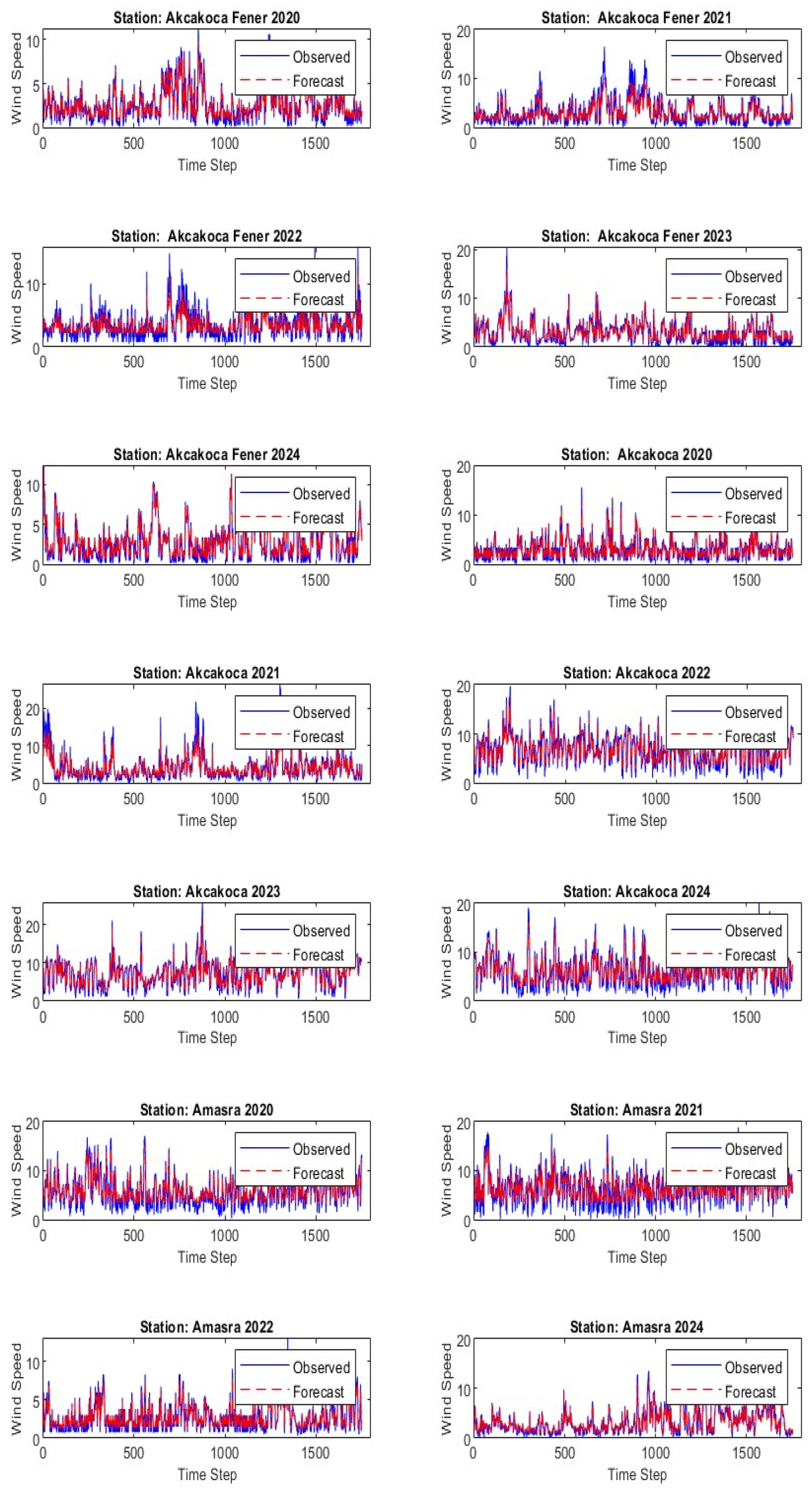
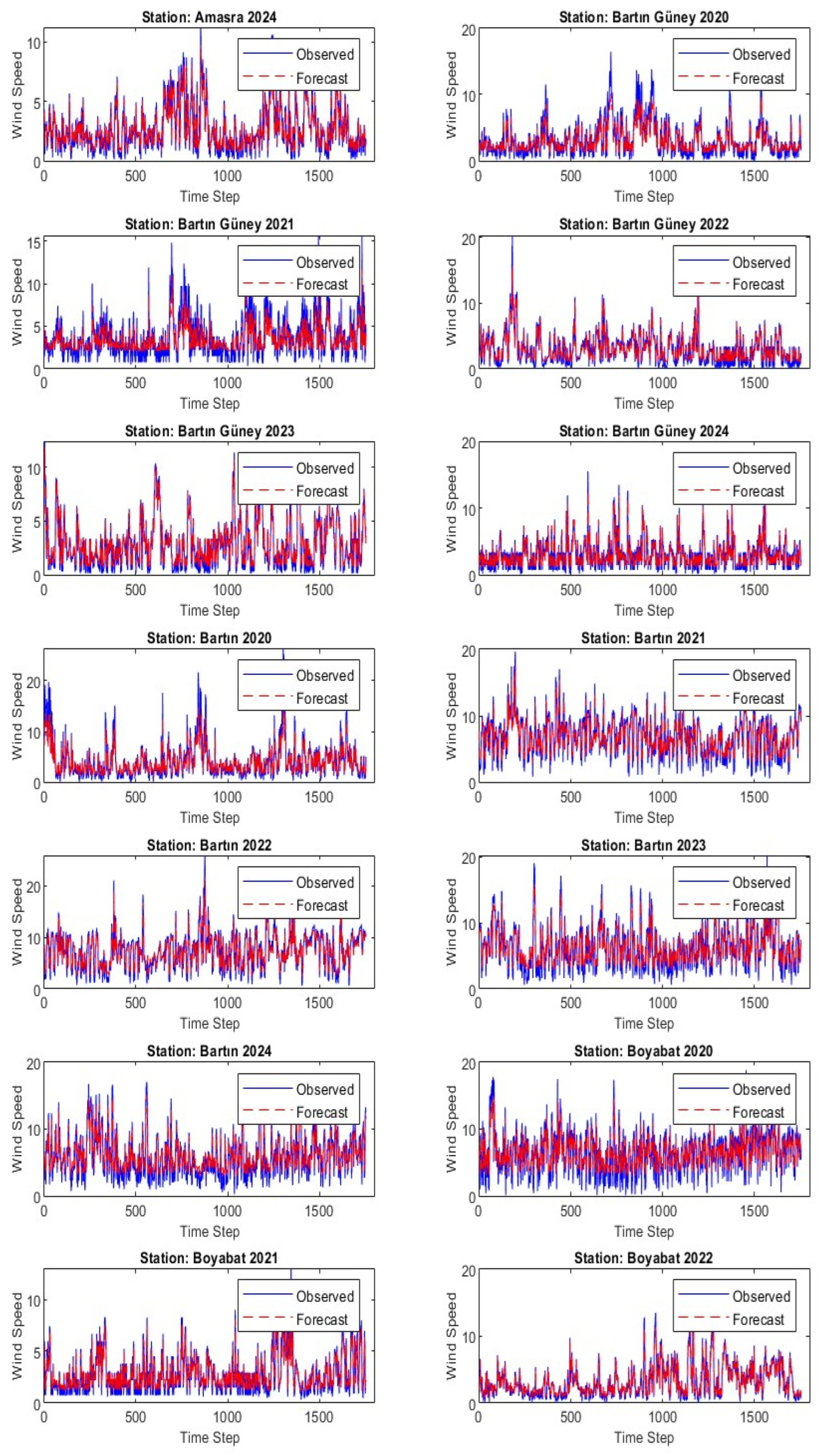
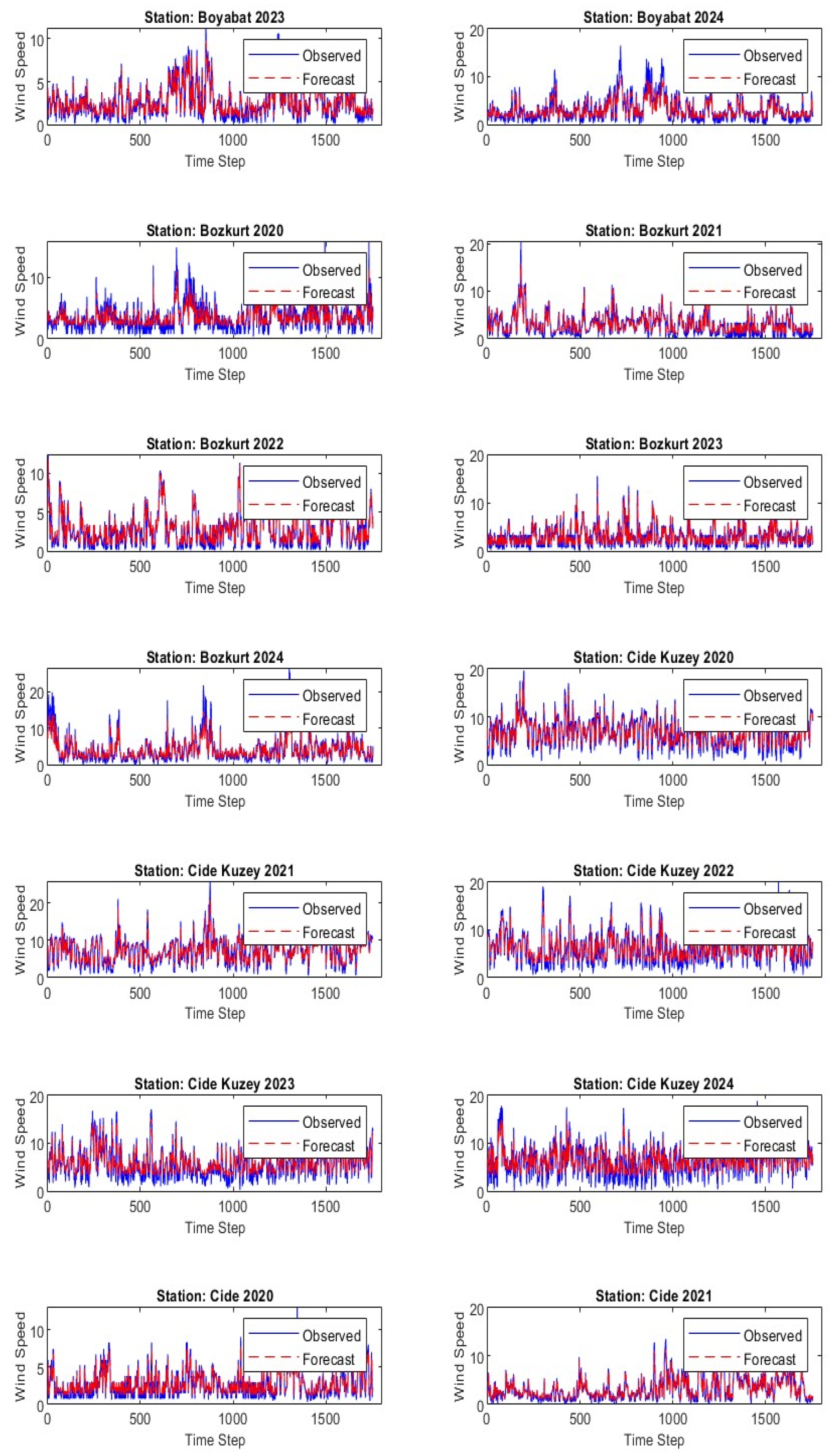
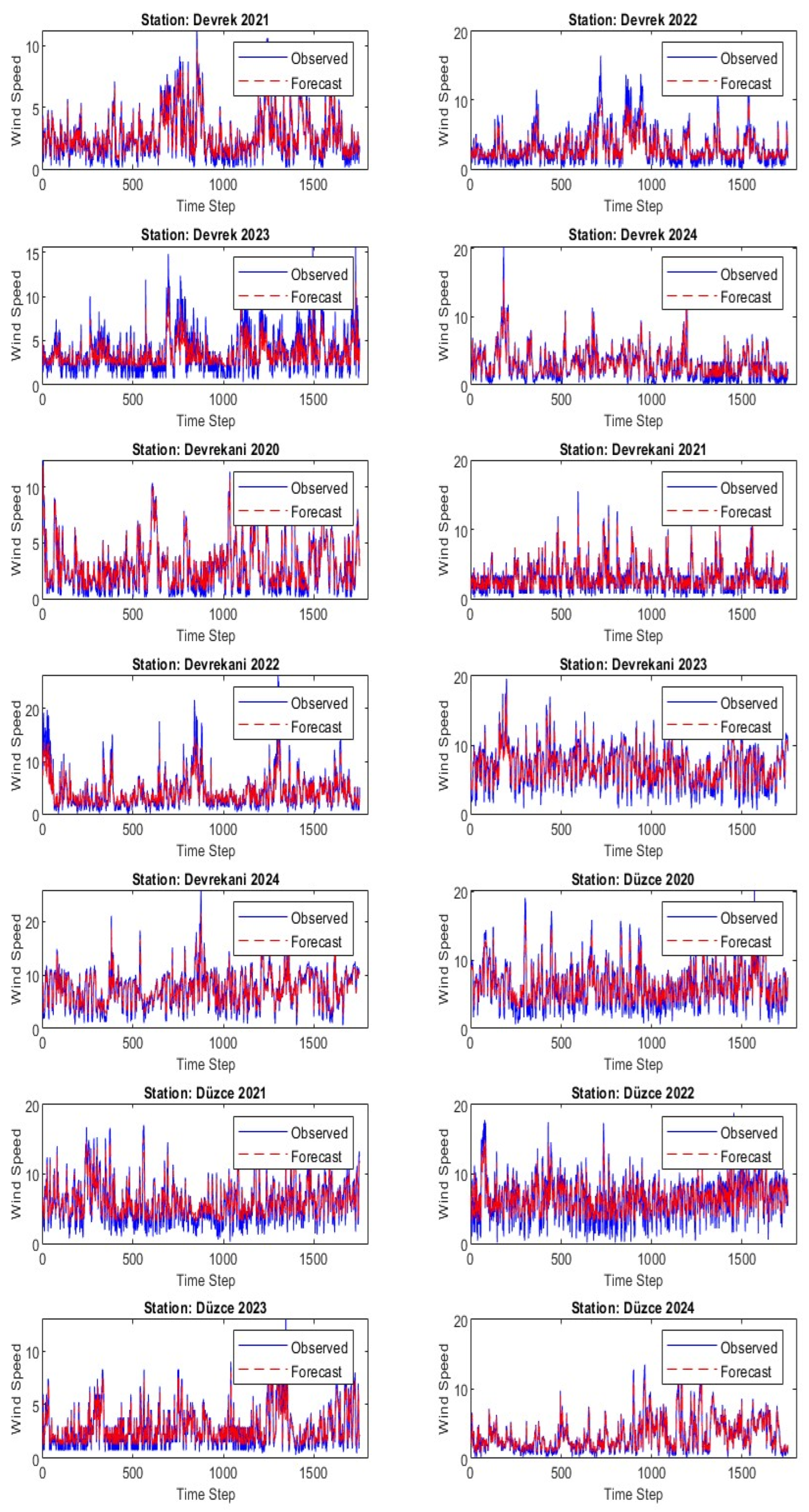
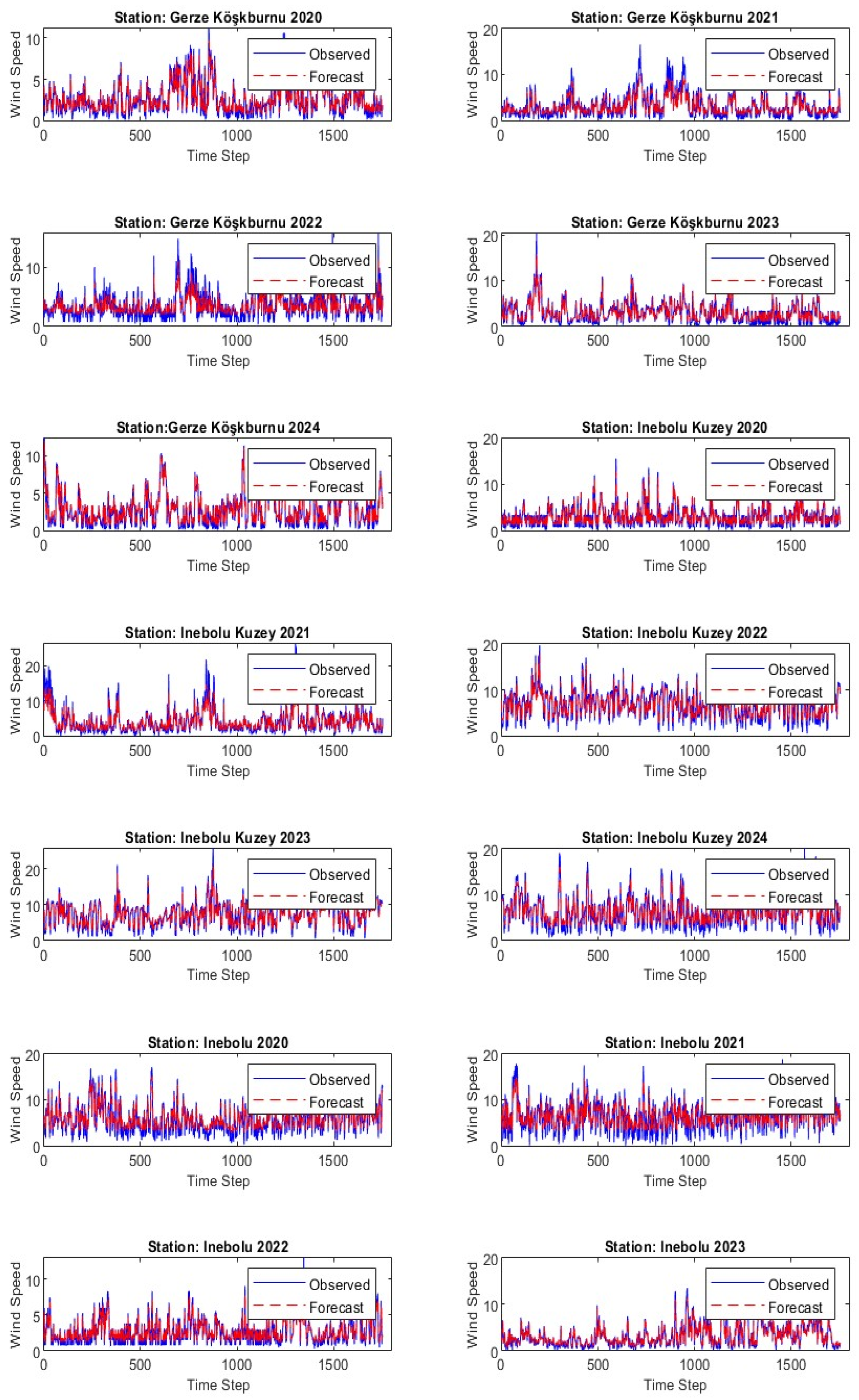
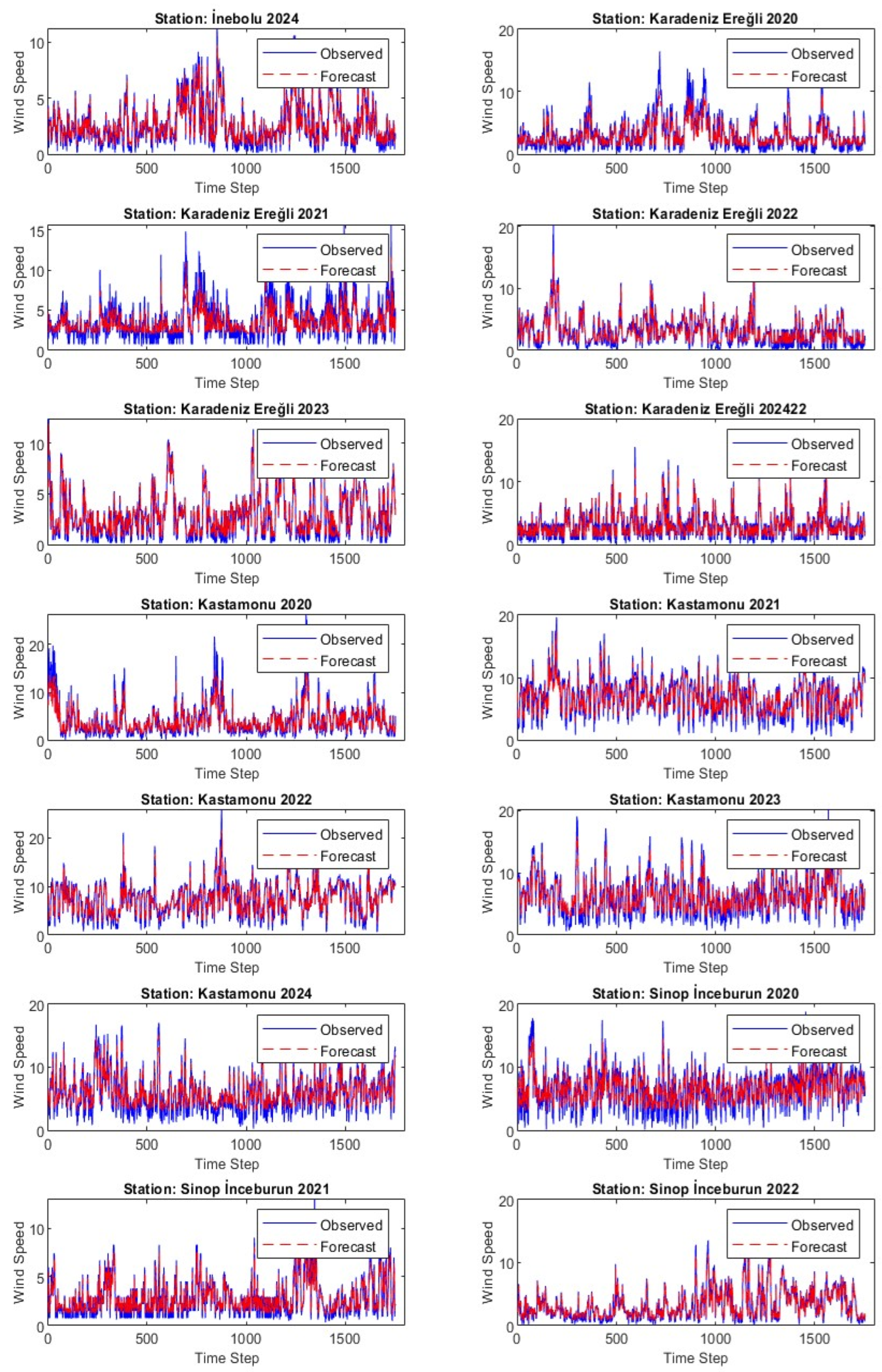
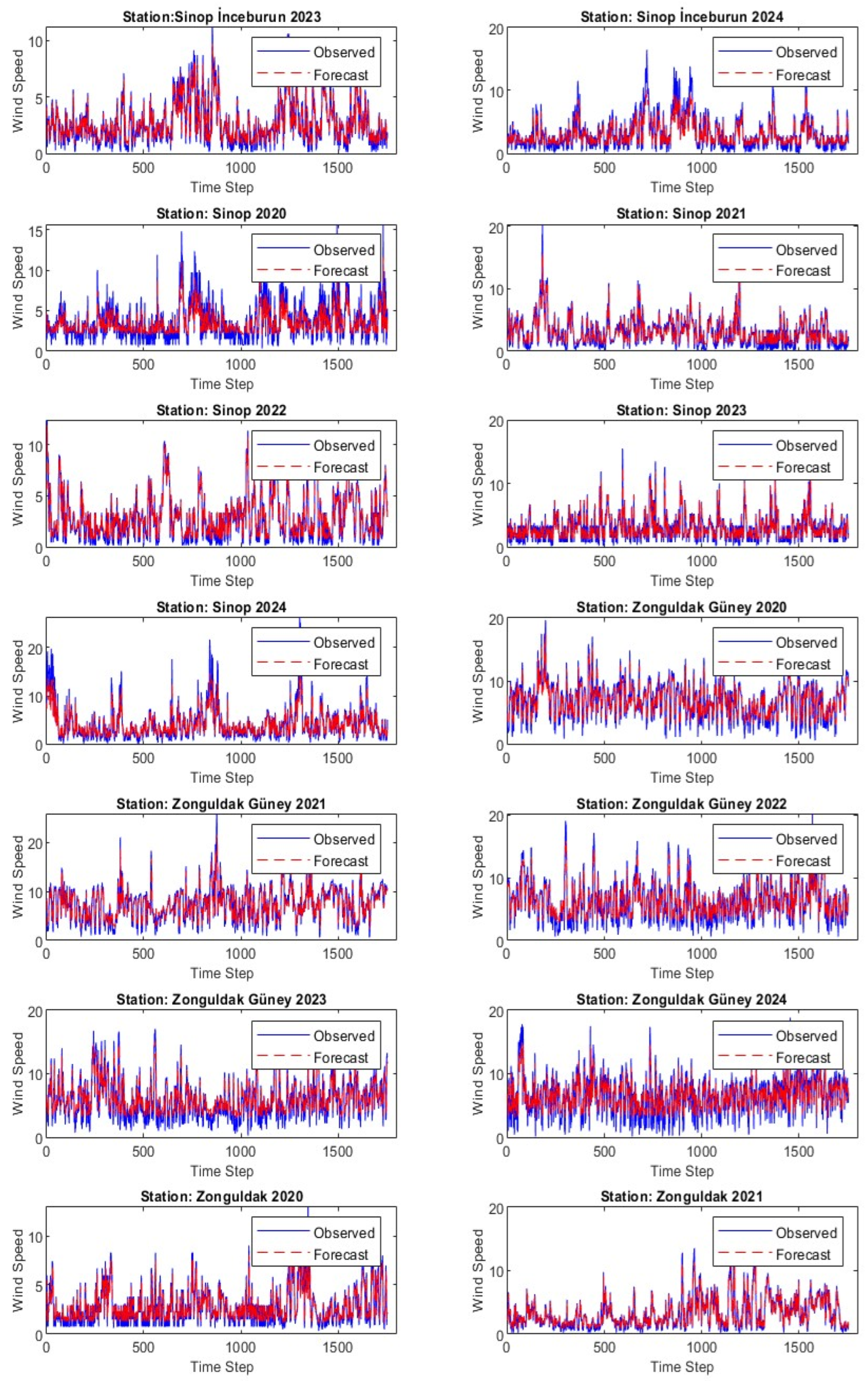
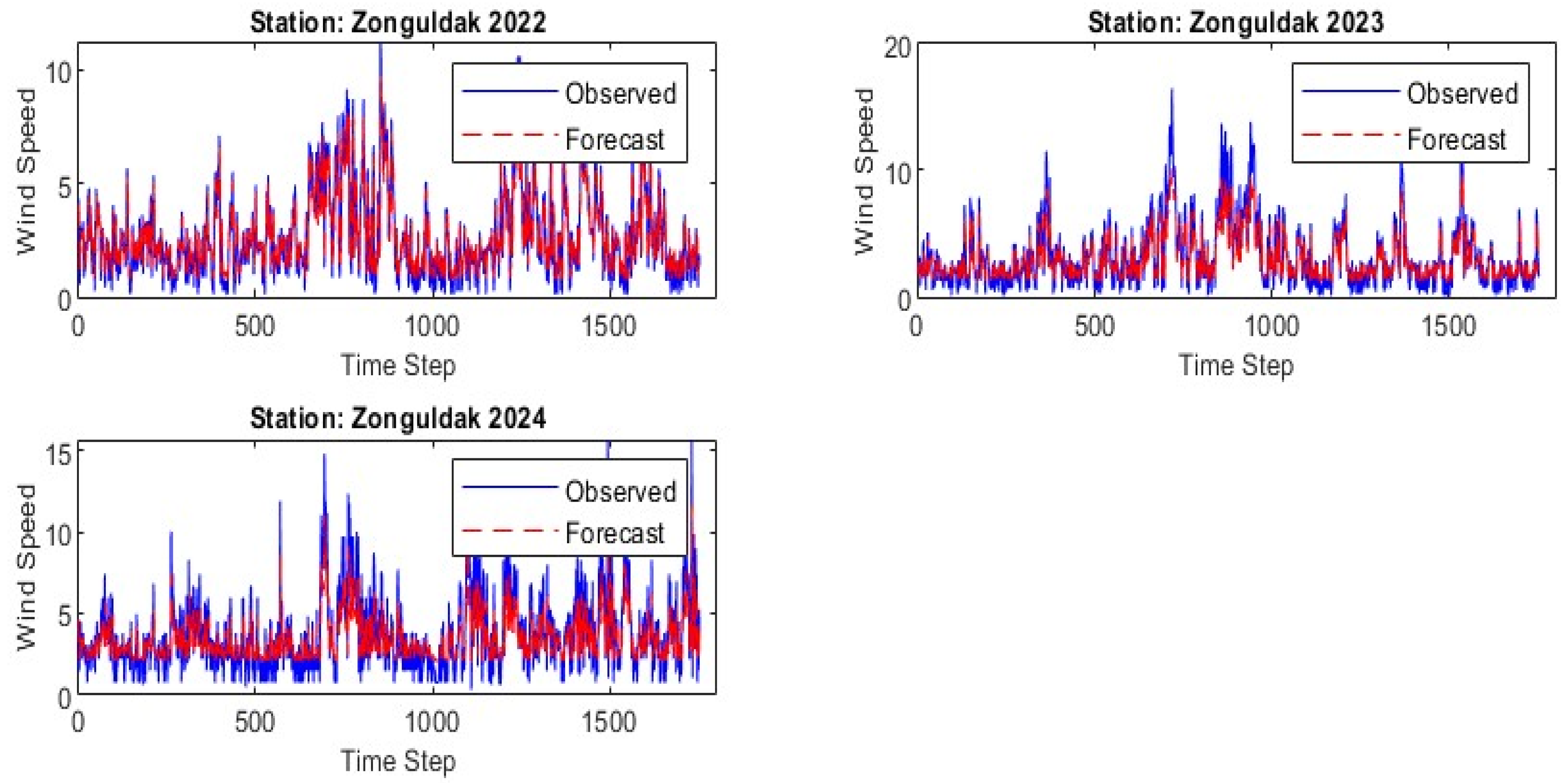
The Weibull parameters were evaluated to determine the wind power density of the regions where wind farms were planned to be established. For this purpose, the Weibull parameter values for the measured data from all stations between the years 2020–2024 were calculated using the wblfit command in the MATLAB R2023b environment. The calculated parameter values are presented in

Table 2. Weibull parameters k and λ for all stations (measured data).

	2020		2021		2022		2023		2024
	λ	k	λ	k	λ	k	λ	k	λ	k
Akçakoca Fener	5.2352	1.5184	5.2863	1.5752	5.1264	1.5454	5.0619	1.5223	3.5191	0.9565
Akçakoca	2.3022	1.7731	1.9750	1.62	1.8819	1.6349	1.8259	1.5098	1.7798	1.4915
Amasra	6.9025	1.6801	7.1793	1.7058	6.5836	1.5779	6.4787	1.4848	6.3312	1.7054
Bartın Güney	8.8973	1.9063	8.9304	2.0551	8.4958	2.0959	8.8964	1.9653	8.7338	2.0213
Bartın	1.7160	1.3175	1.6162	1.2012	1.5973	1.2145	1.7338	1.3249	1.9754	1.5865
Boyabat	1.8410	1.7295	1.8442	1.5914	1.8325	1.6544	1.7942	1.6392	1.8864	1.4883
Bozkurt	2.6415	1.5737	3.3034	1.6278	2.4420	1.5332	2.5205	1.4339	3.8581	1.5728
Cide Kuzey	6.7846	2.0077	7.2135	1.8852	7.0273	1.9132	6.7395	1.7269	6.9692	1.8629
Cide	4.0229	1.3249	4.3878	1.3927	4.1973	1.3620	4.0849	1.2436	4.3649	1.4666
Çatalzeytin	2.9877	1.7574	2.9622	1.751	2.3902	1.3387	2.1447	1.2254	2.2611	1.3855
Devrek Acısu	2.5161	1.6004	3.6001	1.5072	2.9557	1.3387	3.0856	1.3206	2.9640	1.4808
Devrek	1.9084	1.5417	2.0146	1.4969	2.0358	1.4943	2.0899	1.6064	2.1475	1.4962
Devrekani	2.3524	1.2707	3.0625	1.386	2.6900	1.2996	2.9341	1.4095	2.8106	1.4037
Düzce	1.3948	1.5314	0.9414	1.1946	0.9535	1.2570	0.9589	1.4132	1.1523	1.3904
Gerze Köşkburnu	4.6486	1.3208	5.5653	1.4997	6.2263	1.5001	4.8079	1.2417	4.8479	1.2582
İnebolu Kuzey	5.8558	1.5731	6.3520	1.5707	6.1569	1.6266	5.7788	1.4625	5.2540	1.5300
İnebolu	6.7133	1.6685	7.2290	1.696	6.6320	1.5275	7.0996	1.6865	6.8117	1.5873
Karadeniz Ereğli	2.1102	1.4265	2.1074	1.4001	1.8944	1.3503	2.3283	1.5829	2.3327	1.5008
Kastamonu	2.2361	2.0633	2.2831	1.9536	2.2117	2.0340	1.6715	1.4489	1.8226	1.5346
Sinop İnceburun	9.5599	1.8117	9.4001	1.8234	9.7082	1.7800	8.9868	1.7642	9.8999	1.8616
Sinop	4.0414	1.4010	3.2821	1.2003	3.5347	1.2904	3.2647	1.3442	4.4477	1.5992
Zonguldak Güney	7.9006	2.3516	8.0056	2.3731	7.6824	2.3486	7.5157	2.1094	7.6027	2.1560
Zonguldak	3.3865	1.7431	3.3145	1.6222	3.0930	1.5779	3.0758	1.4954	3.6832	1.7977

.

As seen in Equation (10), λ is a determining parameter in wind power density. Upon examining Table 2, the highest λ values were calculated for the Sinop İnceburun, Bartın Güney, and Zonguldak Güney stations. Using the Weibull probability density function, the power density of the area where the wind farm will be established and the annual energy production of the installed turbine can be calculated. Weibull power density can be expressed with the following equation [50].

$$P_w={\displaystyle \frac{1}{2}}{\displaystyle \int \rho }{v}^3{f}_w(v)dv$$

(10)

Here, ρ represents the air density, which has been taken as 1.226 in this study. Considering the swept area depending on the turbine blade length and the number of hours in a year, the annual energy amount can be expressed as follows [36]:

$$E={\displaystyle \frac{1}{2}}{t}_h\rho {\lambda }^3\Gamma \left(1+{\displaystyle \frac{3}{k}}\right)A$$

(11)

Here, A represents the turbine blade swept area, t_h represents the number of hours in a year, and Γ denotes the gamma function. The results obtained from the expression given in Equation (10) were calculated under the assumption that the turbine operates at the same efficiency throughout the year. Therefore, the amount of energy produced by a turbine is also dependent on its efficiency, which is influenced by the capacity factor.

$$CF={\displaystyle \frac{1}{v_m^3}}{\displaystyle \underset{v_c}{\overset{v_r}{\int }}{v}^{3}f(v)dv+}{\displaystyle \underset{v_r}{\overset{v_f}{\int }}f(v)dv}$$

(12)

The capacity factor can be calculated using the formula above [36,51]. Here, CF represents the capacity factor, v is the hourly average wind speed, vm is the mean speed, v_f is the cut-out wind speed, v_c is the cut-in wind speed, and v_r is the rated wind speed. Using Equations (10) and (11), the wind power density for all the stations, the annual energy production of a turbine, and the capacity factor, including the turbine’s annual energy output, are presented in

Table 3. Wind power density, annual energy, and capacity factor, including annual energy amount for all stations (Measured data).

	Power Density					Annual Energy Amount (GW)					Capacity Factor, Including Annual Energy Amount (GW)
	2020	2021	2022	2023	2024	2020	2021	2022	2023	2024	2020	2021	2022	2023	2024
Akçakoca Fener	357.83	345.56	325.63	321.97	1226.48	12.07	11.66	10.98	10.86	41.37	3.02	2.91	2.75	2.72	10.34
Akçakoca	23.88	17.21	14.68	15.34	17.18	0.81	0.58	0.50	0.52	0.58	0.21	0.15	0.13	0.13	0.15
Amasra	694.54	764.26	665.59	706.72	589.57	23.43	25.78	22.45	23.84	19.89	9.37	10.31	8.98	9.54	7.95
Bartın Güney	1258.95	1173.95	991.53	1216.05	1027.92	42.47	39.60	33.45	41.02	34.67	17.84	16.63	14.05	17.23	14.56
Bartın	16.88	17.84	16.71	17.19	9.42	0.57	0.60	0.56	0.58	0.32	0.15	0.16	0.15	0.16	0.09
Boyabat	12.64	14.42	13.30	12.67	15.92	0.43	0.49	0.45	0.43	0.54	0.13	0.15	0.13	0.13	0.16
Bozkurt	43.18	79.92	35.69	44.53	34.15	1.46	2.70	1.20	1.50	1.15	0.51	0.94	0.42	0.53	0.40
Cide Kuzey	527.19	679.76	617.71	621.22	637.53	17.78	22.93	20.84	20.96	21.51	7.11	9.17	8.33	8.38	8.60
Cide	214.73	249.48	229.14	262.54	196.73	7.24	8.42	7.73	8.86	6.64	2.75	3.20	2.94	3.37	2.52
Çatalzeytin	52.82	51.74	43.98	39.50	40.77	1.78	1.75	1.48	1.33	1.38	0.45	0.44	0.37	0.33	0.34
Devrek Acısu	36.29	117.94	83.16	97.63	67.45	1.22	3.98	2.81	3.29	2.28	0.29	0.95	0.67	0.79	0.55
Devrek	16.87	20.93	21.67	20.67	21.62	0.57	0.71	0.73	0.70	0.73	0.17	0.20	0.21	0.20	0.21
Devrekani	47.47	85.70	67.18	72.75	56.54	1.60	2.89	2.27	2.45	1.91	0.48	0.87	0.68	0.74	0.57
Düzce	6.66	3.58	3.25	2.53	2.57	0.22	0.12	0.11	0.09	0.09	0.06	0.03	0.03	0.02	0.02
Gerze Köşkburnu	333.70	439.71	615.43	429.77	902.29	11.26	14.83	20.76	14.50	30.44	3.83	5.04	7.06	4.93	10.35
İnebolu Kuzey	470.76	602.42	518.04	516.21	574.17	15.88	20.32	17.47	17.41	19.37	6.67	8.53	7.34	7.31	8.13
İnebolu	645.65	786.81	719.71	751.50	673.66	21.78	26.54	24.28	25.35	22.72	8.71	10.62	9.71	10.14	9.09
Karadeniz Ereğli	26.41	27.33	21.47	29.28	17.32	0.89	0.92	0.72	0.99	0.58	0.29	0.30	0.23	0.32	0.19
Kastamonu	18.36	20.69	18.02	12.72	26.47	0.62	0.70	0.61	0.43	0.89	0.18	0.20	0.18	0.12	0.26
Sinop İnceburun	1662.04	1567.13	1781.28	1429.99	1682.36	56.06	52.86	60.09	48.24	56.75	22.99	21.67	24.64	19.78	23.27
Sinop	192.51	149.71	155.05	111.03	100.74	6.49	5.05	5.23	3.75	3.40	1.62	1.26	1.31	0.94	0.85
Zonguldak Güney	723.10	747.26	665.46	682.26	714.12	24.39	25.21	22.45	23.01	24.09	10.24	10.59	9.43	9.67	10.12
Zonguldak	77.79	81.17	69.02	74.62	56.86	2.62	2.74	2.33	2.52	1.92	0.79	0.82	0.70	0.76	0.58

.

When examining Table 3, it can be observed that the lowest annual energy production is 0.13 GW at the Akçakoca station, while the highest energy production is 24.64 GW at the Sinop İnceburun site in 2022. At the Sinop İnceburun station, the energy production varies between 19.68 GW and 24.64 GW from 2020 to 2024. Although there is a decrease in 2023, the energy production is generally higher and more stable compared to the other stations. The calculated annual energy production for the Sinop İnceburun, Zonguldak Güney, Bartın Güney, Cide Kuzey, and Amasra stations is notably higher than those of other areas. The highest annual energy productions, including the capacity factor, were observed at the Sinop İnceburun, Bartın Güney, Zonguldak Güney, Amasra, and İnebolu stations. The lowest energy productions were calculated for the Düzce, Boyabat, Bartın, and Devrek stations.

4.2. LSTM Results

Using the parameters provided in Table 3, the LSTM network was trained and the forecasting process was carried out with code developed in the MATLAB R2023b environment. A total of 80% of the hourly wind speed data were used for training, and 20% for testing. The data from all stations for the period of 2020–2024 were used to forecast the period of 2021–2025 using the LSTM method. Examining the error values in

Table 4. Performance values of the LSTM network (RMSE, MAE, and R²).

Stations	2020			2021			2022			2023			2024
	RMSE	MAE	R2	RMSE	MAE	R2	RMSE	MAE	R2	RMSE	MAE	R2	RMSE	MAE	R2
Akçakoca Fener	1.6720	1.1263	0.7832	0.7941	0.5965	0.6201	1.8653	1.2862	0.7712	0.5470	0.2618	0.0412	0.4353	0.3088	0.5504
Akçakoca	1.7756	1.2055	0.7303	0.7551	0.5966	0.2103	1.7089	1.1596	0.743	1.4899	1.0376	0.7665	0.8131	0.6431	0.4383
Amasra	1.4133	0.9795	0.7768	0.3696	0.268	0.5622	2.1388	1.5136	0.4082	1.9377	1.2993	0.683	0.8434	0.6112	0.2262
Bartn Güney	1.7286	1.1077	0.7499	0.4679	0.3166	0.6436	2.1845	1.5261	0.4625	1.9671	1.3627	0.7977	1.5850	1.187	0.8297
Bartın	2.4516	1.7506	0.5674	0.4190	0.2995	0.6424	0.8046	0.5638	0.7809	1.8968	1.3201	0.7295	2.2398	1.4981	0.8067
Boyabat	0.6679	0.4617	0.4992	0.6498	0.445	0.6209	1.1456	0.7827	0.7488	2.5064	1.778	0.4824	1.7305	1.2606	0.8804
Bozkurt	0.7994	0.5221	0.7186	0.9489	0.6503	0.3587	1.1029	0.7655	0.7749	1.6705	1.1935	0.7924	2.3089	1.5666	0.8507
Cide Kuzey	0.5975	0.442	0.5927	1.0366	0.776	0.5357	1.2704	0.8149	0.8257	1.9948	1.3906	0.7759	2.6218	1.9059	0.7673
Cide	1.0724	0.6913	0.5954	2.3049	0.8976	0.5012	1.2168	0.9163	0.6429	1.7332	1.1932	0.7574	1.1713	0.8163	0.7616
Çatalzeytin	0.9893	0.668	0.3749	0.8789	0.6231	0.6367	0.5735	0.4279	0.6029	1.9978	1.4539	0.7353	1.2830	0.9189	0.6901
Devrek Acısu	1.6999	1.2078	0.7992	1.2446	0.8077	0.5569	0.7316	0.5289	0.6358	2.3620	1.7665	0.5197	1.0941	0.7805	0.7653
Devrek	1.9969	1.3973	0.7842	2.0264	1.4505	0.3424	0.7700	0.5811	0.5836	1.7663	1.2663	0.7546	1.5520	1.1116	0.4647
Devrekani	1.7878	1.2442	0.7792	0.9907	0.7185	0.6603	0.7912	0.5486	0.6163	1.8791	1.2952	0.7537	2.0079	1.3502	0.6735
Düzce	2.4247	1.7189	0.7284	1.0229	0.705	0.632	0.9194	0.7377	0.1586	1.7398	1.2043	0.7533	1.5774	1.1773	0.6842
Gerze Köşkburnu	2.5826	1.8324	0.6006	0.9351	0.7273	0.5942	1.1663	0.9197	0.4375	2.2035	1.4917	0.7134	1.8538	1.3119	0.696
İneblu Kuzey	1.8848	1.3894	0.8028	1.0966	0.8558	0.5564	1.1079	0.7528	0.7635	2.7397	1.9759	0.5465	1.7926	1.3134	0.6829
İnebolu	2.0576	1.4411	0.768	1.2506	0.9453	0.2956	1.2151	0.9154	0.7115	0.5758	0.4167	0.7535	1.7006	1.2857	0.6908
Karadeniz Ereğli	1.7907	1.3174	0.7656	1.3899	0.9514	0.7937	1.3408	0.8814	0.756	0.7224	0.5337	0.7487	2.1473	1.6008	0.4743
Kastamonu	1.6921	1.2675	0.7894	1.4287	0.9618	0.794	1.3043	0.9376	0.5353	0.5936	0.4271	0.7176	1.1412	0.8454	0.6214
Sinop İnceburun	2.4617	1.8243	0.6217	1.3015	0.9235	0.7907	0.3377	0.217	0.3738	0.9332	0.5678	0.7553	1.1458	0.8055	0.7668
Sinop	0.6277	0.4485	0.2344	1.6249	1.1566	0.817	0.4548	0.3156	0.6406	1.1746	0.8712	0.3599	0.9745	0.6977	0.7307
Zonguldak Güney	0.6362	0.4214	0.6675	2.1177	1.5629	0.466	0.3713	0.2921	0.4451	0.5329	0.38	0.4086	1.3698	0.9883	0.7093
Zonguldak	0.5976	0.4269	0.5056	1.7772	1.2574	0.6639	0.4428	0.3027	0.5201	0.5032	0.3493	0.663	1.6298	1.1991	0.4865

, the graphs for the four stations with the fewest errors in their predicted values compared to the measured data are presented in Figure 3. The graphs obtained for all the stations are provided additionally (Appendix A).

In Figure 3d, the deviation between the forecast and observed data is seen to be very low. The developed LSTM model significantly predicts both increasing and decreasing trends. In Figure 3a, the sudden rise is not fully predicted, while in Figure 3b and d it is captured well.

In Figure 3a, the 2022 data were predicted using the measured data from 2021 at the Amasra station. Similarly, in Figure 3b–d, the 2023 data were predicted using the 2022 data from the Sinop İnceburun station, the 2023 data for the Bartın station were predicted with the 2022 data, and the 2023 data for the Bozkurt station were predicted based on the 2022 measured wind speed data using LSTM. The performance of the LSTM network used for forecasting from 2021 to 2025 across all the stations was evaluated with RMSE, MAE, and R2 error values. The determined error values are presented in Table 4, and their graphical representation is shown in Figure 4.

Upon examining Table 4 and Figure 4, it can be observed that the RMSE values generally range from 0.3 to 2.7, the MAE values range from 0.2 to 1.9, and the R² values range from 0.04 to approximately 0.9, indicating that the developed LSTM model has a moderate to good prediction accuracy. The highest prediction accuracy was achieved with a 0.3377 error value for the Sinop İnceburun station in 2022. The lowest prediction accuracy, on the other hand, was calculated with a 2.7397 error value for the İnebolu Kuzey station in 2023. Similarly, according to the MAE criterion, the lowest error was recorded for the Sinop İnceburun station in 2020, while the highest error was recorded for the Cide Kuzey station in 2024. To evaluate the prediction error among the stations, the distribution of the observed and forecast error values for each station, along with error boxplots, are presented in Figure 5.

Upon examining Figure 5, it can be observed that, for station 81, there are no outliers in the observed and forecasted data. For station 84, there is 1 outlier in the forecasted data, while 25 outliers exist in the observed data. For station 79, 20 outliers are identified in the observed data, but no outliers are detected in the forecasted data. There are fewer than 10 outliers in the forecasted data 10 for stations 8, 12, 36, 58, 59, 79, 80, 81, 83, and 84. In the distribution of the measured data, stations 25, 29, 30, 40, 60, 61, 91, 92, and 93, and in the distribution of the forecasted data, stations 26, 27, 28, 29, 66, 67, 68, 69, 91, 92, and 93, have much smaller IQR (Inter Quartile Range) values compared to the other stations. Hourly wind speed data were analyzed using the Maximum Likelihood Estimation method, and the shape and scale parameters of the Weibull distribution were determined. Based on the analysis of the wind speed data forecasted using the LSTM model in MATLAB R2023b, the computed parameter values are provided in

Table 5. k and λ parameters for all stations (forecast data).

Year	2020		2021		2022		2023		2024
Stations	λ	k	λ	k	λ	k	λ	k	λ	k
Akçakoca Fener	4.9817	1.6762	4.5572	1.5999	7.4169	2.1041	5.0352	2.3896	3.8361	2.9029
Akçakoca	3.5460	1.8956	1.7718	2.8574	2.0104	2.2298	2.3565	1.5370	2.4490	1.7952
Amasra	6.8018	1.8067	6.3623	2.5606	6.5689	2.6573	6.3817	1.9881	6.7421	3.0618
Bartın Güney	8.2861	1.7717	8.4108	2.0186	8.3711	2.6680	8.4379	1.6384	8.5310	2.3671
Bartın	2.2011	1.5590	1.3648	2.1472	3.2785	2.0043	4.8683	1.5596	2.5479	1.9050
Boyabat	1.9411	2.1992	1.5502	2.0483	1.5424	1.6628	1.6928	1.7645	1.1943	1.8046
Bozkurt	2.0887	1.7714	2.7820	2.3978	2.8210	1.7652	2.5567	1.7063	2.3297	1.8840
Cide Kuzey	6.8741	2.4246	6.9673	2.2485	7.1525	1.7419	6.6667	1.7536	6.8468	1.9948
Cide	3.0381	1.8316	3.0253	2.0044	3.2491	1.9970	4.5084	1.7490	3.3281	1.5802
Çatalzeytin	1.7948	2.1821	2.3191	1.8542	1.7171	2.1195	2.1754	1.8012	2.3754	1.6747
Devrek Acısu	2.1432	1.9614	2.8302	2.1666	1.9380	1.8434	2.7306	2.0970	3.0626	1.5865
Devrek	1.9897	2.0191	1.7631	2.6487	2.1290	1.9685	2.1277	2.1428	2.0279	1.7768
Devrekani	1.7333	1.8323	2.0999	2.2539	2.0541	2.2113	2.1588	2.1451	2.7046	1.7807
Düzce	1.6594	1.8956	1.9769	1.0112	1.8986	1.0284	1.5529	1.3440	1.7166	1.3539
Gerze Köşkburnu	4.9046	1.1249	5.1755	1.8286	6.2180	1.8627	4.6951	1.4655	4.6464	1.8396
İnebolu Kuzey	5.0260	1.2109	5.3002	1.8843	5.2443	1.5760	5.2537	1.2615	5.2490	1.7708
İnebolu	6.2947	1.2845	6.2996	1.0204	6.8608	1.4314	6.7909	1.6974	6.9311	1.7051
Karadeniz Ereğli	2.3024	1.5344	2.1970	1.5215	2.4640	1.6790	2.3181	1.8888	2.3963	1.3701
Kastamonu	2.4609	1.1954	2.4991	1.6033	2.8303	1.9781	1.9264	1.9333	2.2045	1.0141
Sinop İnceburun	9.5166	1.7874	10.1004	1.5333	8.8927	1.2373	8.3058	1.7226	9.6427	1.6803
Sinop	4.3779	2.1534	3.2964	1.6264	3.8728	1.5425	3.3632	2.3052	4.1062	1.8566
Zonguldak Güney	7.3331	1.4604	7.7764	2.1496	7.5873	2.0063	7.3019	1.8658	7.4670	1.8395
Zonguldak	2.2207	1.6510	3.6607	2.4361	2.8680	1.9387	3.0163	2.5915	3.4772	2.5881

.

Upon examining Table 1 and Table 5, it is evident that the Weibull parameters of the measured and forecasted wind data are highly consistent. Based on the parameters of the forecasted data, wind power density, annual energy production potential, and annual energy output, including the capacity factor, were calculated. The results are presented in

Table 6. Annual energy output including wind power density, annual energy, and capacity factor based on forecasted data (using LSTM predictions).

	Power Density					Annual Energy Amount (GW)					Capacity Factor, Including Annual Energy Amount (GW)
	2021	2022	2023	2024	2025	2021	2022	2023	2024	2025	2021	2022	2023	2024	2025
Akçakoca Fener	262.01	215.75	657.27	184.99	527.81	8.84	7.28	22.17	6.24	17.80	2.21	1.82	5.54	1.56	4.45
Akçakoca	80.22	7.25	12.43	31.93	15.64	2.71	0.24	0.42	1.08	0.53	0.70	0.06	0.11	0.28	0.14
Amasra	600.76	356.32	383.65	443.31	358.38	20.26	12.02	12.94	14.95	12.09	8.11	4.81	5.18	5.98	4.84
Bartın Güney	1035.74	998.75	792.17	1318.38	855.94	34.94	33.69	26.72	44.47	28.87	14.67	14.15	11.22	18.68	12.13
Bartın	25.39	4.02	59.59	274.50	63.04	0.86	0.14	2.01	9.26	2.13	0.23	0.04	0.54	2.50	0.57
Boyabat	11.32	6.16	7.87	9.56	7.02	0.38	0.21	0.27	0.32	0.24	0.11	0.06	0.08	0.10	0.07
Bozkurt	17.85	31.12	44.20	34.50	40.69	0.60	1.05	1.49	1.16	1.37	0.21	0.37	0.52	0.41	0.48
Cide Kuzey	445.82	513.72	733.62	588.60	621.89	15.04	17.33	24.75	19.85	20.98	6.02	6.93	9.90	7.94	8.39
Cide	52.61	46.82	58.23	182.69	79.81	1.77	1.58	1.96	6.16	2.69	0.67	0.60	0.75	2.34	1.02
Çatalzeytin	9.01	23.05	8.10	19.73	10.74	0.30	0.78	0.27	0.67	0.36	0.08	0.19	0.07	0.17	0.09
Devrek Acısu	17.04	35.55	13.55	32.90	16.82	0.57	1.20	0.46	1.11	0.57	0.14	0.29	0.11	0.27	0.14
Devrek	13.22	7.43	16.64	15.26	18.83	0.45	0.25	0.56	0.51	0.64	0.13	0.07	0.16	0.15	0.18
Devrekani	9.76	14.04	13.35	15.92	16.86	0.33	0.47	0.45	0.54	0.57	0.10	0.14	0.14	0.16	0.17
Düzce	8.22	56.70	47.23	11.95	21.49	0.28	1.91	1.59	0.40	0.72	0.07	0.48	0.40	0.10	0.18
Gerze Köşkburnu	467.71	260.61	441.71	275.76	448.56	15.78	8.79	14.90	9.30	15.13	5.36	2.99	5.07	3.16	5.14
İnebolu Kuzey	524.82	269.80	337.10	538.48	282.74	17.70	9.10	11.37	18.16	9.54	7.44	3.82	4.78	7.63	4.01
İnebolu	885.51	1774.62	901.27	651.47	667.39	29.87	59.86	30.40	21.98	22.51	11.95	23.94	12.16	8.79	9.00
Karadeniz Ereğli	29.87	26.35	31.62	22.51	45.76	1.01	0.89	1.07	0.76	1.54	0.32	0.28	0.34	0.24	0.49
Kastamonu	63.82	35.46	38.88	12.57	164.63	2.15	1.20	1.31	0.42	5.55	0.62	0.35	0.38	0.12	1.61
Sinop İnceburun	1515.79	2525.29	2744.67	1166.92	1484.91	51.13	85.18	92.58	39.36	50.09	20.96	34.93	37.96	16.14	20.54
Sinop	132.30	79.52	140.86	56.64	107.15	4.46	2.68	4.75	1.91	3.61	1.12	0.67	1.19	0.48	0.90
Zonguldak Güney	973.55	742.65	737.86	713.87	815.01	32.84	25.05	24.89	24.08	27.49	13.79	10.52	10.45	10.11	11.55
Zonguldak	23.75	70.12	41.36	37.69	32.43	0.80	2.37	1.40	1.27	1.09	0.24	0.71	0.42	0.38	0.33

.

When examining Table 6, it can be observed that the calculated annual energy values are close to those calculated in Table 2. Similarly to Table 2, the highest energy productions in Table 6 are also calculated for the Sinop İnceburun, Zonguldak Güney, and Bartın Güney stations. The highest energy production, including the capacity factor, was determined for the Sinop İnceburun station in 2023, with a value of 37.96 GW. The lowest energy production occurred at the Düzce station in 2022, with a value of 0.07 GW. This indicates that the method used effectively predicts wind speed data.

4.3. Economical Analysis Results

In this study, the wind energy investment potential of five coastal cities in Türkiye’s Western Black Sea Region was examined. In the first phase, the electrical potential that could be obtained from wind power was predicted using the Weibull and LSTM methods. In the second phase, economic analysis of the investment project was conducted. In both the technical and economic analyses, wind turbines with a capacity of 1000 kW were utilized. Cost, volume, and profit analyses for WPPs with a total installed capacity of 10 MW, consisting of 10 turbines, each with a capacity of 1000 kW, were carried out.

Previous studies indicate that the evaluation of WPP investment projects involves costs such as investment costs, operating costs, maintenance and repair costs, and insurance costs [32,52]. At the beginning of the project, costs are high, but they may decrease in the later stages. In WPP investment projects, costs are generally categorized as investment and operating costs. The investment cost of a wind energy plant can be calculated using the following Formula (13):

$$InvestmentCost=FeasibilityCosts+InvestmentCosts+OperatingCost$$

(13)

When preparing a WPP investment project, the first step is identifying the region where the wind farm will be established. To determine the wind power, measurement devices are placed on poles at specific heights to obtain real-time wind power data. Wind power measurements typically take about one year. During this phase, the potential electricity supply that can be generated from wind energy is predicted using various methods. Cost, volume, and profit analyses of the obtained data are conducted, and a project decision is made. All costs incurred during this phase constitute the feasibility and project costs.

The investment costs associated with a wind power plant (WPP) encompass a range of components, including land acquisition, wind turbine procurement, installation, construction, transportation, facility setup, licensing, and other related expenses. Among these, the purchase, transportation, and installation of wind turbines constitute the largest share of the overall investment. Notably, wind turbine costs vary significantly depending on the capacity and specifications of the turbine. When examining the costs of investment projects, it has been noted that the cost of a 1000 kW capacity plant is approximately USD 1.93 million [28]. It was estimated that the investment cost of a 1000 kW turbine in Türkiye would amount to approximately USD 11.92 million by 2024. The estimated cost for a wind power plant consisting of 1000 kW turbines is based on price data obtained from the Soyutwind company [53]. The investment cost was recalculated for the period of 2021–2024, adjusted for inflation. The investment cost is determined by including turbines, inverters, transportation, construction, installation expenses, project costs, and taxes. Since the completion of the wind energy investment project requires a long period, the capital cost must also be included in the calculation [54]. Inflation and interest rates are used in the investment cost calculations [30,55,56]. Additionally, the cost of the land where the plant will be located should be included in investment cost analysis. However, since WPPs are typically established in rural areas in Türkiye, land costs are not expected to be high. Reference [57] states that 30% of the investment cost consists of land and other investments. Estimated land costs are included in the investment costs.

After the completion of the WPP investment project, the operation phase begins. During this phase, operational costs emerge. [30] states that the annual operating and maintenance cost of the plant constitutes 25% of the wind turbines’ investment cost, and when calculating, the useful life of the turbines is taken into account. The average useful life of wind turbines is said to be about 20 years [58]. It is observed that depreciation amounts are not taken into account when calculating wind energy investment costs [55,56]. However, even though depreciation is not considered as an expense item, it must be included when calculating cash flows, as depreciation plays an important role in determining the value of a company’s assets [59]. The cash flow amount is calculated by adding the net profit at the end of the period, as well as depreciation. Cost, volume, and profit analyses are performed using the following formulas:

$$AnnualCosts=\left(InvestmentCost/UsefulLife\right)+OperatingExpenses$$

(14)

$$TotalRevenues=TotalElectricityProduction\left(gW\right)\times ElectricitySalePrice$$

(15)

$$TotalProfit/Loss=TotalRevenues–AnnualCosts$$

(16)

$$UnitCost\left(perkWh\right)=AnnualExpenses/AnnualElectricityProductionAmount$$

(17)

$$UnitProfit/Loss\left(perkWh\right)=UnitRevenue-UnitCost$$

(18)

Annual costs are calculated by dividing the investment cost by the useful life of the wind energy plant and adding the operating expenses (Formula (14)). Total revenues are calculated by multiplying the electricity production amount by the electricity sale price (Formula (15)). The annual profit or loss are obtained by subtracting the total costs from the total revenues (Formula (16)). Unit cost (per kWh) is determined by dividing the annual expenses by the annual electricity production amount (Formula (17)). Unit profit or loss (per kWh) is calculated by subtracting the unit cost from the unit revenue (Formula (18)).

In Türkiye, the electricity generated from wind energy is supported by the government. The electricity purchase price for 2020 was given in TRY. To convert it into USD, the exchange rate of The Central Bank of the Republic of Türkiye (CBRT) on 19 November 2020 was used [60]. The payment for electricity was approximately 0.0139 USD/kWh for 2020, 0.0510 USD/kWh for the 2021 and 2022 periods, and 0.0605 USD/kWh for the 2023–2025 period [61,62,63]. Various indicators are used during the establishment of a WPP. In the economic analysis calculations, since there is a possibility of the depreciation of the TRY, calculations were made in USD to avoid the impact of exchange rate risk. For calculating the capital cost during the 2020–2025 period, interest rates (1.75–4.5%) were used, and inflation rates (1.4–7.0%) were utilized to calculate the investment amount accurately [64]. The useful life of the wind energy investment project was set at 20 years. The annual operation and maintenance cost was calculated as 30% of the annual investment cost. The initial costs, such as land allocation, installation, construction, and project expenses, were calculated as 30% of the turbine amount. The annual expenses were recalculated according to the inflation rate for the 2020–2024 period. During this period, sales revenues were discounted according to the risk-free interest rate, and the alternative returns on investment for each year were added to the sales revenues. This approach aimed to preserve the real value of income against inflation. The annual cash inflows for each station were calculated using Microsoft Excel. As part of the economic analysis, the observed and forecast values for each year, including unit revenue, cost, and profits, were calculated.

The economic analysis findings for the observed electricity production values for the year 2020 are provided in

Table 7. The 2020 economic analysis findings.

Stations	Power Plant Electricity Production (gW)	Total Revenue (USD/gW)	Total Cost USD/gW	Total Net Profit/Loss (USD/gW)	Unit Revenue (USD/kWh)	Unit Cost (USD/kWh)	Unit Net Profit/Loss (USD/kWh)
Akçakoca Fener	30.20	418,783	827,180	−408,397	0.0139	0.0274	−0.0135 *
Akçakoca	2.10	29,121	788,214	−759,093	0.0139	0.3753	−0.3615 *
Amasra	93.70	1,299,338	915,235	384,102	0.0139	0.0098	0.0041
Bartın Güney	178.40	2,473,873	1,032,689	1,441,184	0.0139	0.0058	0.0081
Bartın	1.50	20,801	787,382	−766,581	0.0139	0.5249	−0.5111 *
Boyabat	1.30	18,027	787,104	−769,077	0.0139	0.6055	−0.5916 *
Bozkurt	5.10	70,722	792,374	−721,652	0.0139	0.1554	−0.1415 *
Cide Kuzey	71.10	985,944	883,896	102,048	0.0139	0.0124	0.0014
Cide	27.50	381,343	823,436	−442,093	0.0139	0.0299	−0.0161 *
Çatalzeytin	4.50	62,402	791,542	−729,140	0.0139	0.1759	−0.1620 *
Devrek Acısu	2.90	40,214	789,323	−749,109	0.0139	0.2722	−0.2583 *
Devrek	1.70	23,574	787,659	−764,085	0.0139	0.4633	−0.4495 *
Devrekâni	4.80	66,562	791,958	−725,396	0.0139	0.1650	−0.1511 *
Düzce	0.60	8,320	786,134	−777,813	0.0139	1.3102	−1.2964 *
Gerze Köşkburnu	38.30	531,106	838,412	−307,306	0.0139	0.0219	−0.0080 *
İnebolu Kuzey	66.70	924,929	877,795	47,134	0.0139	0.0132	0.0007
İnebolu	87.10	1,207,816	906,083	301,732	0.0139	0.0104	0.0035
Karadeniz Ereğli	2.90	40,214	789,323	−749,109	0.0139	0.2722	−0.2583 *
Kastamonu	1.80	24,961	787,798	−762,837	0.0139	0.4377	−0.4238 *
Sinop İnceburun	229.90	3,188,023	1,104,104	2,083,919	0.0139	0.0048	0.0091
Sinop	16.20	224,645	807,766	−583,121	0.0139	0.0499	−0.0360 *
Zonguldak Güney	102.40	1,419,981	927,300	492,681	0.0139	0.0091	0.0048
Zonguldak	7.90	109,549	796,257	−686,707	0.0139	0.1008	−0.0869 *

Note: * indicates that a WPP is not suitable.

.

According to the economic analysis findings based on the observed electricity generation potential for the year 2020, losses were incurred at 16 stations due to costs exceeding revenues. It was concluded that wind energy investment at these stations is not rational. However, at seven stations, revenues were found to be higher than costs. The stations with the highest revenues were Sinop İnceburun (USD 3,188,023), Bartın Güney (USD 2,473,873), and Zonguldak Güney (USD 1,419,981). In comparison to other stations, it is anticipated that wind energy investments could be feasible at the Bartın Güney, Sinop İnceburun, and Zonguldak Güney stations. For the remaining four stations, considering the economic lifespan of the investment, it is believed that the investment would not be rational. When examining the unit electricity generation values, the highest profits were observed in the following order: Sinop İnceburun (0.0091 USD/kWh), Bartın Güney (0.0081 USD/kWh), and Zonguldak Güney (0.0048 USD/kWh).

The findings of the economic analysis for the observed and forecast projected electricity generation values for 2021 are presented in

Table 8. Economic analysis findings for 2021.

	Power Plant Electricity Generation (GW))		Total Revenue (USD/GW)		Total Cost (USD/GW)		Total Net Profit/Loss (USD/GW)		Unit Cost (USD/kWh)		Unit Net Profit/Loss (USD/kWh)
Stations	Observed	Forecast	Observed	Forecast	Observed	Forecast	Observed	Forecast	Observed	Forecast	Observed	Forecast
Akçakoca-Fener	29.10	22.10	1,457,910	306,461	947,023	868,463	510,887	−562,002	0.0325	0.0393	0.0176	−0.0254 *
Akçakoca	1.50	7.00	75,150	97,069	808,747	835,778	−733,597	−738,709	0.5392	0.1194	−0.4891 *	−0.1055 *
Amasra	103.10	81.10	5,165,310	1,124,614	1,317,763	938,532	3,847,547	186,081	0.0128	0.0116	0.0373	0.0023
Bartın-Güney	166.30	146.70	8,331,630	2,034,289	1,634,395	1,029,500	6,697,235	1,004,789	0.0098	0.0070	0.0403	0.0068
Bartın	1.60	2.30	80,160	139,150	809,248	839,986	−729,088	−700,836	0.5058	0.3652	−0.4557 *	−0.3047 *
Boyabat	1.50	1.10	75,150	15,254	808,747	827,596	−733,597	−812,343	0.5392	0.7524	−0.4891 *	−0.7385 *
Bozkurt	9.40	2.10	470,940	29,121	848,326	828,983	−377,386	−799,862	0.0902	0.3948	−0.0401 *	−0.3809 *
Cide Kuzey	91.70	60.20	4,594,170	834,793	1,260,649	909,550	3,333,521	−74,757	0.0137	0.0151	0.0364	−0.0012 *
Cide	32.00	6.70	1,603,200	92,909	961,552	835,362	641,648	−74.453	0.0300	0.1247	0.0201	−0.1108 *
* Çatalzeytin	4.40	0.80	220,440	11,094	823,276	827,180	−602,836	−816,087	0.1871	1.0340	−0.1370 *	−1.0201 *
Devrek-Acısu	9.50	1.40	475,950	19,414	848,827	828,012	−372,877	−808,598	0.0894	0.5914	−0.0393 *	−0.5776 *
Devrek	2.00	1.30	100,200	18,027	811,252	827,874	−711,052	−809,847	0.4056	0.6368	−0.3555 *	−0.6230 *
Devrekâni	8.70	1.00	435,870	13,867	844,819	827,458	−408,949	−813,591	0.0971	0.8275	−0.0470 *	−0.8136 *
Düzce	0.30	0.70	15,030	9,707	802,735	827,042	−787,705	−817,335	2.6758	1.1815	−2.6257 *	−1.1676 *
Gerze-Köşkburnu	50.40	53.60	2,525,040	743,271	1,053,736	900,398	1,471,304	−157,127	0.0209	0.0168	0.0292	−0.0029 *
İnebolu Kuzey	85.30	74.40	4,273,530	1,031,705	1,228,585	929,241	3,044,945	102,463	0.0144	0.0125	0.0357	0.0014
İnebolu	106.20	119.50	5,320,620	1,657,107	1,333,294	991,782	3,987,326	665,325	0.0126	0.0083	0.0375	0.0056
Karadeniz-Ereğli	3.00	3.20	150,300	44,374	816,262	830,508	−665,962	−786,134	0.2721	0.2595	−0.2220 *	−0.2457 *
Kastamonu	2.00	6.20	100,200	85,975	811,252	834,668	−711,052	−748,693	0.4056	0.1346	−0.3555 *	−0.1208 *
Sinop-İnceburun	239.80	209.60	10,856,670	2,906,523	1,886,899	1,116,723	8,969,771	1,789,800	0.0087	0.0053	0.0414	0.0085
Sinop	12.60	11.20	631,260	155,310	864,358	841,602	−233,098	−686,292	0.0686	0.0751	−0.0185 *	−0.0613 *
Zonguldak Güney	105.90	137.90	5,305,590	1,912,259	1,331,791	1,017,297	3,973,799	894,962	0.0126	0.0074	0.0375	0.0065
Zonguldak	8.20	2.40	410,820	33,281	842,314	829,399	−431,494	−796,118	0.1027	0.3456	−0.0526 *	−0.3317 *

Note: * indicates that a WPP is not suitable.

.

According to the economic analysis findings for the observed electricity generation values in 2021, losses were observed at 13 stations where costs exceeded revenues, while, based on the forecasted values, losses were identified at 17 stations. Upon examining the observed values, the highest revenues were generated at the Sinop İnceburun (USD 10,856,670), Bartın Güney (USD 8,331,630, and İnebolu (USD 5,320,620) stations. Based on the forecasted values, the highest revenues were forecasted for the Sinop İnceburun (USD 2,906,523), Bartın Güney (USD 2,034,289), and Zonguldak Güney (USD 1,912,259) stations.

When examining the unit values of the observed electricity production, the highest profits were recorded in the following order: Sinop İnceburun (0.0414 USD/kWh), Bartın Güney (0.0403 USD/kWh), İnebolu, and Zonguldak Güney (0.0375 USD/kWh). For the forecasted values, the highest profits were forecasted for the Sinop İnceburun (0.0085 USD/kWh), Bartın Güney (0.0068 USD/kWh), and Zonguldak Güney (0.0065 USD/kWh) stations.

According to the findings of the economic analysis based on the observed values, the stations with the highest profitability potential were determined to be Sinop İnceburun, Bartın Güney, and Zonguldak Güney. It is forecasted that wind energy investment would be rational at these stations. However, considering net profit and investment profitability at the other three stations, it is believed that wind energy investment at those sites would not be rational.

The economic analysis findings for the observed and forecasted electricity generation values for the year 2022 are presented in

Table 9. Economic analysis findings for 2022.

	Power Plant Electricity Generation (GW)		Total Revenue (USD/GW)		Total Cost (USD/GW)		Total Net Profit/Loss (USD/GW)		Unit Cost (USD/kWh)		Unit Net Profit/Loss (USD/kWh)
Stations	Observed	Forecast	Observed	Forecast	Observed	Forecast	Observed	Forecast	Observed	Forecast	Observed	Forecast
Akçakoca-Fener	27.50	18.20	1,377,750	911,820	995,094	945,832	382,656	−34,012	0.0362	0.0520	0.0139	−0.0019 *
Akçakoca	1.30	0.60	65,130	30,060	863,832	840,642	−798,702	−810,582	0.6645	1.4011	−0.6144 *	−1.3510 *
Amasra	89.80	48.10	4,498,980	2,409,810	1,307,217	1,078,617	3,191,763	1.331,193	0.0146	0.0224	0.0355	0.0277
Bartın-Güney	140.50	141.50	7,039,050	7,089,150	1,561,224	1,546,551	5,477,826	5,542,599	0.0111	0.0109	0.0390	0.0392
Bartın	1.50	0.40	75,150	24,200	864,834	840,056	−789,684	−815,856	0.5766	2.1001	−0.5265 *	−2.0396 *
Boyabat	1.30	0.60	65,130	30,060	863,832	840,642	−798,702	−810,582	0.6645	1.4011	−0.6144 *	−1.3510 *
Bozkurt	4.20	3.70	210,420	185,370	878,361	856,173	−667,941	−670,803	0.2091	0.2314	−0.1590 *	−0.1813 *
Cide Kuzey	83.30	69.30	4,173,330	3,471,930	1,274,652	1,184,829	2,898,678	2,287,101	0.0153	0.0171	0.0348	0.0330
Cide	29.40	6.00	1,472,940	300,600	1,004,613	867,696	468,327	−567,096	0.0342	0.1446	0.0159	−0.0945 *
Çatalzeytin	3.70	1.90	185,370	95,190	875,856	847,155	−690,486	−751,965	0.2367	0.4459	−0.1866 *	−0.3958 *
Devrek-Acısu	6.70	2.90	335,670	145,290	890,886	852,165	−555,216	−706,875	0.1330	0.2938	−0.0829 *	−0.2437 *
Devrek	2.10	0.70	105,210	35,070	867,840	841,143	−762,630	−806,073	0.4133	1.2016	−0.3632 *	−1.1515 *
Devrekâni	6.80	1.40	340,680	70,140	891,387	844,650	−550,707	−774,510	0.1311	0.6033	−0.0810 *	−0.5532 *
Düzce	0.30	4.80	15,030	240,480	858,822	861,684	−843,792	−621,204	2.8627	0.1795	−2.8126 *	−0.1294 *
Gerze-Köşkburnu	70.60	29.90	3,537,060	1,497,990	1,211,025	987,435	2,326,035	510,555	0.0172	0.0330	0.0329	0.0171
İnebolu Kuzey	73.40	38.20	3,677,340	1,913,820	1,225,053	1,029,018	2,452,287	884,802	0.0167	0.0269	0.0334	0.0232
İnebolu	97.10	239.40	4,864,710	11,993,940	1,343,790	2,037,030	3,520,920	9,956,910	0.0138	0.0085	0.0363	0.0416
Karadeniz-Ereğli	2.30	2.80	115,230	140,280	868,842	851,664	−753,612	−711,384	0.3778	0.3042	−0.3277 *	−0.2541 *
Kastamonu	1.80	3.50	90,180	175,350	866,337	855,171	−776,157	−679821	0.4813	0.2443	−0.4312 *	−0.1942 *
Sinop-İnceburun	246.40	349.30	12,344,640	17,499,930	2,091,783	2,587,629	10,252,857	14,912,301	0.0085	0.0074	0.0416	0.0427
Sinop	13.10	6.70	656,310	335,670	922,950	871,203	−266,640	−535,533	0.0705	0.1300	−0.0204 *	−0.0799 *
Zonguldak Güney	94.30	105.20	4724,430	5,270,520	1,329,762	1,364,688	3,394,668	3,905,832	0.0141	0.0130	0.0360	0.0371
Zonguldak	7.00	7.10	350,700	355,710	892,389	873,207	−541,689	−517,497	0.1275	0.1230	−0.0774 *	−0.0729 *

Note: * indicates that a WPP is not suitable.

.

According to the economic analysis findings for the observed electricity generation values in 2022, losses were observed at 13 stations where costs exceeded revenues. Based on the forecasted values, losses were identified at 16 stations. Upon examining the observed values, the highest revenues were generated at the Sinop İnceburun (USD 12,344,640), Bartın Güney (USD 7,039,050), and İnebolu (USD 4,864,710) stations. According to the forecasted values, the highest revenues were forecasted for Sinop İnceburun (USD 17,499,930), İnebolu (USD 11,993,940), and Bartın Güney (USD 7,089,150) stations.

When examining the unit values of the observed electricity production, the highest profits were recorded in the following order: Sinop İnceburun (0.0416 USD/kWh), Bartın Güney (0.0390 USD/kWh), and İnebolu (0.0363 USD/kWh). For the forecasted values, the highest profits were forecasted for the Sinop İnceburun (0.0427 USD/kWh), İnebolu (0.0416 USD/kWh), and Zonguldak Güney (0.0392 USD/kWh) stations.

According to the economic analysis findings based on the observed values, the stations with the highest profitability potential were identified as Sinop İnceburun, Bartın Güney, İnebolu, Zonguldak Güney, Amasra, Cide Kuzey, İnebolu Kuzey, and Gerze Köşkburnu. It is forecasted that wind energy investment would be rational at these stations. However, based on net profit and investment profitability, it is believed that wind energy investment would not be rational at the other two stations.

According to the economic analysis findings based on the forecasted values, the stations with the highest profitability potential were identified as Sinop İnceburun, İnebolu, Bartın Güney, Cide Kuzey, and Amasra. It is forecasted that wind energy investment would be rational at these stations.

The economic analysis findings for the observed and forecast electricity generation values for the year 2023 are presented in

Table 10. Economic analysis findings for 2023.

	Power Plant Electricity Generation (GW)		Total Revenue (USD/GW)		Total Cost (USD/GW)		Total Net Profit/Loss (USD/GW)		Unit Cost (USD/kWh)		Unit Net Profit/Loss (USD/kWh)
Stations	Observed	Forecast	Observed	Forecast	Observed	Forecast	Observed	Forecast	Observed	Forecast	Observed	Forecast
Akçakoca-Fener	27.20	55.40	1,645,600	2,775,540	1,092,605	1,192,030	552,995	1,583,510	0.0402	0.0215	0.0203	0.0286
Akçakoca	1.30	1.10	78,650	55,110	935,910	901,781	−857,260	−846,671	0.7199	0.8198	−0.6594 *	−0.7697 *
Amasra	95.40	51.80	5,771,700	2,595,180	1,505,215	1,155,788	4,266,485	1,439,392	0.0158	0.0223	0.0447	0.0278
Bartın-Güney	172.30	112.20	10,424,150	5,621,220	1,970,460	1,458,392	8,453,690	4,162,828	0.0114	0.0130	0.0491	0.0371
Bartın	1.60	5.40	96,800	326,700	937,725	928,940	−840,925	−602,240	0.5861	0.1720	−0.5256 *	−0.1115 *
Boyabat	1.30	0.80	78,650	40,080	935,910	900,278	−857,260	−860,198	0.7199	1.1253	−0.6594 *	−1.0752 *
Bozkurt	5.30	5.20	320,650	260,520	960,110	922,322	−639,460	−661,802	0.1812	0.1774	−0.1207 *	−0.1273 *
Cide Kuzey	83.80	99.00	5,069,900	4,959,900	1,435,035	1,392,260	3,634,865	3,567,640	0.0171	0.0141	0.0434	0.0360
Cide	33.70	7.50	2,038,850	375,750	1,131,930	933,845	906,920	−558,095	0.0336	0.1245	0.0269	−0.0744 *
* Çatalzeytin	3.30	0.70	199,650	35,070	948,010	899,777	−748,360	−864,707	0.2873	1.2854	−0.2268 *	−1.2353 *
Devrek-Acısu	7.90	1.10	477,950	55,110	975,840	901,781	−497,890	−846,671	0.1235	0.8198	−0.0630 *	−0.7697 *
Devrek	2.00	1.60	121,000	80,160	940,145	904,286	−819,145	−824,126	0.4701	0.5652	−0.4096 *	−0.5151 *
Devrekâni	7.40	1.40	447,700	70,140	972,815	903,284	−525,115	−833,144	0.1315	0.6452	−0.0710 *	−0.5951 *
Düzce	0.20	4.00	12,100	200,400	929,255	916,310	−917,155	−715,910	4.6463	0.2291	−4.5858 *	−0.1790 *
Gerze-Köşkburnu	49.30	50.70	2,982,650	2,540,070	1,226,310	1,150,277	1,756,340	1,389,793	0.0249	0.0227	0.0356	0.0274
İnebolu Kuzey	73.10	47.80	4,422,550	2,394,780	1,370,300	1,135,748	3,052,250	1,259,032	0.0187	0.0238	0.0418	0.0263
İnebolu	101.40	121.60	6,134,700	6,092,160	1,541,515	1,505,486	4,593,185	4,586,674	0.0152	0.0124	0.0453	0.0377
Karadeniz-Ereğli	3.20	3.40	193,600	170,340	947,405	913,304	−753,805	−742,964	0.2961	0.2686	−0.2356 *	−0.2185 *
Kastamonu	1.20	3.80	72,600	190,380	935,305	915,308	−862,705	−724,928	0.7794	0.2409	−0.7189 *	−0.1908 *
Sinop-İnceburun	197.80	379.60	11,966,900	19,017,960	2,124,735	2,798,066	9,842,165	16,219,894	0.0107	0.0074	0.0498	0.0427
Sinop	9.40	11.90	568,700	596,190	984,915	955,889	−416,215	−359,699	0.1048	0.0803	−0.0443 *	−0.0302 *
Zonguldak Güney	96.70	104.50	5,850,350	5,235,450	1,513,080	1,419,815	4,337,270	3,815,635	0.0156	0.0136	0.0449	0.0365
Zonguldak	7.60	4.20	459,800	210,420	974,025	917,312	−514,225	−706,892	0.1282	0.2184	−0.0677 *	−0.1683 *

Note: * indicates that a WPP is not suitable.

.

According to the economic analysis findings for the observed electricity generation values in 2023, losses were observed at 13 stations where costs exceeded revenues. Based on the forecasted values, losses were identified at 14 stations. Upon examining the observed values, the highest revenues were generated at the Sinop İnceburun (USD 11,966,900), Bartın Güney (USD 10,424,150), and İnebolu (USD 6,134,700) stations. According to the forecasted values, the highest revenues were forecasted for the Sinop İnceburun (USD 19,017,960), İnebolu (USD 6,092,160), and Bartın Güney (USD 5,621,220) stations.

When examining the unit values of the observed electricity production, the highest profits were recorded in the following order: Sinop İnceburun (0.0498 USD/kWh), Bartın Güney (0.0491 USD/kWh), and İnebolu (0.0453 USD/kWh). For the forecasted values, the highest profits were forecasted for the Sinop İnceburun (0.0427 USD/kWh), İnebolu (0.0377 USD/kWh), and Bartın Güney (0.0371 USD/kWh) stations.

According to the economic analysis findings based on the observed values, the stations with the highest profitability potential were identified as Sinop İnceburun, Bartın Güney, İnebolu, Zonguldak Güney, Amasra, Cide Kuzey, İnebolu Kuzey, and Gerze Köşkburnu. It is forecasted that wind energy investment would be rational at these stations. However, based on net profit and investment profitability, it is believed that wind energy investment would not be rational at the Cide and Akçakoca Fener stations.

According to the economic analysis findings based on the forecasted values, the stations with the highest profitability potential were identified as Sinop İnceburun, İnebolu Kuzey, İnebolu, Bartın Güney, Zonguldak Güney, Cide Kuzey, Akçakoca Fener, Amasra, and Gerze Köşkburnu. It is forecasted that wind energy investment would be rational at these stations. Based on the LSTM forecast results, the successful outcome of investment being rational at every station where unit profit exists may serve as evidence for the accuracy of the approach.

The economic analysis findings for the observed and forecasted electricity generation values for the year 2024 are presented in

Table 11. Economic analysis findings for 2024.

	Power Plant Electricity Generation (GW)		Total Revenue (USD/GW)		Total Cost (USD/GW)		Total Net Profit/Loss (USD/GW)		Unit Cost (USD/kWh)		Unit Net Profit/Loss (USD/kWh)
Stations	Observed	Forecast	Observed	Forecast	Observed	Forecast	Observed	Forecast	Observed	Forecast	Observed	Forecast
Akçakoca-Fener	103.40	15.60	6,255,700	943,800	1,585,169	1,083,808	4,670,531	−140,008	0.0153	0.0695	0.0452	−0.0090 *
Akçakoca	1.50	2.80	90,750	169,400	968,674	971,468	−877,924	−802,068	0.6458	0.3470	−0.5853 *	−0.2865 *
Amasra	79.50	59.80	4,809,750	3,617,900	1,440,574	1,316,318	3,369,176	2,301,582	0.0181	0.0220	0.0424	0.0385
Bartın-Güney	145.60	186.80	8,808,800	11,301,400	1,840,479	2,084,668	6,968,321	9,216,732	0.0126	0.0112	0.0479	0.0493
Bartın	0.90	25.00	54,450	1,512,500	965,044	1,105,778	−910,594	406,722	1.0723	0.0442	−1.0118 *	0.0163
Boyabat	1.60	1.00	96,800	60,500	969,279	960,578	−872,479	−900,078	0.6058	0.9606	−0.5453 *	−0.9001 *
Bozkurt	4.00	4.10	242,000	248,050	983,799	979,333	−741,799	−731,283	0.2459	0.2389	−0.1854 *	−0.1784 *
Cide Kuzey	86.00	79.40	5,203,000	4,803,700	1,479,899	1,434,898	3,723,101	3,368,802	0.0172	0.0181	0.0433	0.0424
Cide	25.20	23.40	1,524,600	1,415,700	1,112,059	1,096,098	412,541	319,602	0.0441	0.0468	0.0164	0.0137
* Çatalzeytin	3.40	1.70	205,700	102,850	980,169	964,813	−774,469	−861,963	0.2883	0.5675	−0.2278 *	−0.5070 *
Devrek-Acısu	5.50	2.70	332,750	163,350	992,874	970,863	−660,124	−807,513	0.1805	0.3596	−0.1200 *	−0.2991 *
Devrek	2.10	1.50	127,050	90,750	972,304	963,603	−845,254	−872,853	0.4630	0.6424	−0.4025 *	−0.5819 *
Devrekâni	5.70	1.60	344,850	96,800	994,084	964,208	−649,234	−867,408	0.1744	0.6026	−0.1139 *	−0.5421 *
Düzce	0.20	1.00	12,100	60,500	960,809	960,578	−948,709	−900,078	4.8040	0.9606	−4.7435 *	−0.9001 *
Gerze-Köşkburnu	103.50	31.60	6,261,750	1,911,800	1,585,774	1,145,708	4,675,976	766,092	0.0153	0.0363	0.0452	0.0242
İnebolu Kuzey	81.30	76.30	4,918,650	4,616,150	1,451,464	1,416,143	3,467,186	3,200,007	0.0179	0.0186	0.0426	0.0419
İnebolu	90.90	87.90	5,499,450	5,317,950	1,509,544	1,486,323	3,989,906	3,831,627	0.0166	0.0169	0.0439	0.0436
Karadeniz-Ereğli	1.90	2.40	114,950	145,200	971,094	969,048	−856,144	−823,848	0.5111	0.4038	−0.4506 *	−0.3433 *
Kastamonu	2.60	1.20	157,300	72,600	975,329	961,788	−818,029	−889,188	0.3751	0.8015	−0.3146 *	−0.7410 *
Sinop-İnceburun	232.70	161.40	14,078,350	9,764,700	2,367,434	1,930,998	11,710,916	7,833,702	0.0102	0.0120	0.0503	0.0485
Sinop	8.50	4.80	514,250	290,400	1,011,024	983,568	−496,774	−693,168	0.1189	0.2049	−0.0584 *	−0.1444 *
Zonguldak Güney	101.20	101.10	6,122,600	6,116,550	1,571,859	1,566,183	4,550,741	4,550,367	0.0155	0.0155	0.0450	0.0450
Zonguldak	5.80	3.80	350,900	229,900	994,689	977,518	−643,789	−747,618	0.1715	0.2572	−0.1110 *	−0.1967 *

Note: * indicates that a WPP is not suitable.

.

Based on the results of the analysis based on the observed and forecasted values for the year 2024, losses were observed at 13 stations where costs exceeded revenues. Upon examining the observed values, the highest revenues were generated at the Sinop İnceburun (USD 14,078,350), Bartın Güney (USD 8,808,800), and Gerze Köşkburnu (USD 6,261,750) stations. Based on the forecasted values, the highest revenues were forecasted for the Bartın Güney (USD 11,301,400), Sinop İnceburun (USD 9,764,700), and Zonguldak Güney (USD 6,112,600) stations.

When examining the unit values of the observed electricity production, the highest profits were recorded in the following order: Sinop İnceburun (0.0503 USD/kWh), Bartın Güney (0.0479 USD/kWh), and Akçakoca Fener and Gerze Köşkburnu (0.0452 USD/kWh) stations. For the forecasted values, the stations with the highest profits were Bartın Güney (0.0493 USD/kWh), Sinop İnceburun (0.0485 USD/kWh), and Zonguldak Güney (0.0450 USD/kWh).

According to the economic analysis findings based on the observed values, the stations with the highest profitability potential were identified as Sinop İnceburun, Bartın Güney, Gerze Köşkburnu, Akçakoca Fener, Zonguldak Güney, Cide Kuzey, İnebolu, İnebolu Kuzey, and Amasra. It is forecasted that wind energy investment would be rational at these stations. However, based on net profit and investment profitability, it is believed that wind energy investment would not be rational at the Cide station.

In the economic analysis findings based on the forecasted values, the stations with the highest profitability potential were identified as Bartın Güney, Sinop İnceburun, Zonguldak Güney, İnebolu, Cide Kuzey, İnebolu Kuzey, and Amasra. It is forecasted that wind energy investment would be rational at these stations. However, wind energy investment is considered unsuitable at the Gerze Köşkburnu, Bartın, and Cide stations.

The economic analysis findings for the projected annual electricity generation for the year 2025 are presented in

Table 12. Economic analysis findings for 2025.

Stations	Power Plant Electricity Generation (GW)	Total Revenue (USD/GW)	Total Cost (USD/GW)	Total Net Profit/Loss (USD/GW)	Unit Revenue (USD/kWh)	Unit Cost (USD/kWh)	Unit Net Profit/Loss (USD/kWh)
Akçakoca Fener	44.50	2,692,250	1,303,177	1,389,073	0.0605	0.0293	0.0312
Akçakoca	1.40	84,700	1,005,952	−921,252	0.0605	0.7185	−0.6580 *
Amasra	48.40	2,928,200	1,290,302	1,637,898	0.0605	0.0267	0.0338
Bartın Güney	121.30	7,338,650	1,731,347	5,607,303	0.0605	0.0143	0.0462
Bartın	5.70	344,850	1,031,967	−687,117	0.0605	0,1810	−0.1205 *
Boyabat	0.70	42,350	1,001,717	−959,367	0.0605	1.4310	−1.3705 *
Bozkurt	4.80	290,400	1,026,522	−736,122	0.0605	0.2139	−0.1534 *
Cide Kuzey	83.90	5,075,950	1,505,077	3,570,873	0.0605	0.0179	0.0426
Cide	10.20	617,100	1,059,192	−442,092	0.0605	0.1038	−0.0433 *
Çatalzeytin	0.90	54,450	1,002,927	−948,477	0.0605	1.1144	−1.0539 *
Devrek Acısu	1.40	84,700	1,005,952	−921,252	0.0605	0.7185	−0.6580 *
Devrek	1.80	108,900	1,008,372	−899,472	0.0605	0.5602	−0.4997 *
Devrekani	1.70	102,850	1,007,767	−904,917	0.0605	0.5928	−0.5323 *
Düzce	1.80	108,900	1,008,372	−899,472	0.0605	0.5602	−0.4997 *
Gerze Köşkburnu	51.40	3,109,700	1,308,452	1,801,248	0.0605	0.0255	0.0350
İnebolu Kuzey	40.10	2,426,050	1,240,087	1,185,963	0.0605	0.0309	0.0296
İnebolu	90.00	5,445,000	1,541,982	3,903,018	0.0605	0.0171	0.0434
Karadeniz Ereğli	4.90	296,450	1,027,127	−730,677	0.0605	0.2096	−0.1491 *
Kastamonu	16.10	974,050	1,094,887	−120,837	0.0605	0.0680	−0.0075 *
Sinop İnceburun	205.40	12,426,700	2,240,152	10,186,548	0.0605	0.0109	0.0496
Sinop	9.00	544,500	1,051,932	−507,432	0.0605	0.1169	−0.0564 *
Zonguldak Güney	115.50	6,987,750	1,696,257	5,291,493	0.0605	0.0147	0.0458
Zonguldak	3.30	199,650	1,017,447	−817,797	0.0605	0.3083	−0.2478 *

Note: * indicates that a WPP is not suitable.

.

According to the economic analysis findings of the electricity generation forecast for the year 2025, losses were identified at 14 stations where costs exceeded revenues. The analysis results indicated that the highest revenues would be obtained from the Sinop İnceburun (USD 12,426,700), Bartın Güney (USD 7,338,650), and Zonguldak Güney (USD 6,987,750) stations. When examining the unit values of electricity production, it was predicted that the highest profits would be obtained from the Sinop İnceburun (0.0496 USD/kWh), Bartın Güney (0.0462 USD/kWh), and Zonguldak Güney (0.0458 USD/kWh) stations.

As indicated the economic analysis findings, the stations with the highest profitability potential in 2025 were identified as Sinop İnceburun, Bartın Güney, Zonguldak Güney, İnebolu, Cide Kuzey, Gebze Köşkburnu, and Amasra. When considering the net profit and investment amounts for the Akçakoca Fener and İnebolu Kuzey stations, the payback period for investment was found to be longer than 10 years. Therefore, investing in these stations might depend on the investor’s decision. According to the LSTM analysis findings, it is believed that all the stations showing net profit in 2025 are suitable for wind energy investment.

This study evaluated hourly wind speed data collected from 23 different stations located along the northwestern coastline of Türkiye in the Western Black Sea Region. Wind speed data from 2020 to 2024 were forecasted using the LSTM method. The observed and forecasted data were analyzed using the Weibull distribution, and the annual energy production potential of the stations was determined. As a result of the Weibull analysis of the observed data, the highest annual energy production occurred at the Sinop İnceburun station, with 24.64 GW in 2022. The lowest energy production was calculated for the Düzce station. In the Weibull analysis of the forecasted data, the highest energy production was forecasted at Sinop İnceburun, with 37.96 GW in 2022, while the lowest energy production (0.06 GW) occurred at the Akçakoca and Boyabat stations in 2022. The lowest forecast error was 0.3713, and the highest forecast error was 2.7397. Since the RMSE, MAE, and R² values for the all stations fall between these two values, the network’s performance is considered moderately good. The forecasted values followed the observed values, with the least deviation at the Zonguldak Güney station. It was observed that the forecasted values successfully followed the trends at approximately 89% of the stations, while in 11% of the stations, forecasting was less successful.

After determining the potential energy that could be generated from wind power, an economic analysis of the observed and forecasted values was carried out. The observed values for 2020 were initially analyzed. The economic analysis of the observed and forecasted values for 2021–2024 was then conducted. In 2025, economic analysis was performed based on the LSTM method, and the forecast results were provided. The highest revenue in 2020 was realized at the Sinop İnceburun station, and it is predicted that the highest revenue in 2025 will also occur at this station. According to the economic analysis findings, stations where investments can be made have been identified.

5. Discussion

This study analyzed the hourly wind data from 23 measurement stations located in Türkiye’s Western Black Sea Region between 2020 and 2024 using the Weibull distribution. First, the parameters of the two-parameter Weibull distribution were determined. The scale parameter (λ) is a significant determinant of the region’s wind power density. In the analysis, the highest λ values were determined for the Sinop İnceburun, Bartın Güney, and Zonguldak Güney areas. Using the Weibull distribution parameters, the wind power potential of each location, the annual energy production of a turbine, and the annual energy production capacity, including the capacity factor, were calculated. The highest production in 2022 was calculated for Sinop İnceburun, with 24.64 GW, while the lowest production was calculated for Akçakoca station with 0.13 GW. Significant results were obtained in Sinop İnceburun, Zonguldak Güney, Bartın Güney, Cide Kuzey, and Amasra compared to other stations.

Hourly average wind speed data measured at all stations between 2020 and 2024 were used to construct an LSTM network in MATLAB R2023b, with 80% of the data used for training and 20% for testing. The forecasted hourly average wind speed data for the following year was predicted. Observed and forecasted data were compared. Additionally, the forecasted data for the years 2021–2025 were reanalyzed using the Weibull distribution, and the parameters of the distribution, wind power density, and annual energy production capacity, including the capacity factor, were determined. When comparing the annual energy production including the capacity factor for the observed and forecasted data, the highest production was calculated for the Bartın Güney, Sinop İnceburun, and Zonguldak Güney stations in both analyses.

The economic analysis revealed interesting findings. In 2020, the highest revenue of USD 3.18 million was achieved at the Sinop İnceburun station, with a unit energy cost of 0.0048 USD/kWh and a unit electricity profit of 0.0091 USD/kWh. When comparing the observed and forecasted values in 2021, it was observed that the LSTM method did not predict the observed values accurately. In 2021, the observed revenue at Sinop İnceburun was USD 10.8 million, while the forecasted value was USD 2.9 million. The unit electricity profit was 0.0374 USD/kWh based on the observed values and 0.0085 USD/kWh based on the forecasted values. In 2022, however, it was found that the prediction accuracy of the LSTM method increased, with the forecasted values closer to the observed values, and at some stations, the forecast exceeded the observed values. At the Bartın Güney station, the observed revenue was USD 7.03 million, while the forecasted value was USD 7.08 million. The highest unit profit of 0.0427 USD/kWh was forecasted at Sinop İnceburun in 2022. In 2023, it was predicted that the highest revenue of USD 19.01 million would come from the Sinop İnceburun station using LSTM. In 2024, the highest unit profit of 0.0493 USD/kWh was calculated for the Bartın Güney station. It was predicted that investment could be made at all stations with a profit in 2025. The highest unit profit of 0.0496 USD/kWh was forecasted for 2025. Unit costs were anticipated to range between 0.0109 USD/kWh and 1.4310 USD/kWh.

In the city of Deokjeok-do, South Korea, the potential for WPP investment was researched, and the unit cost of electricity was determined to be 0.077 EUR/kWh [26]. In [27], the cost of energy derived from wind power ranged between 0.0259 USD/kWh and 0.0498 USD/kWh at the best location, while at the worst location, it was found to be 0.222 USD/kWh. It was stated that energy costs ranged between 0.056 USD/kWh and 0.074 USD/kWh [28]. In Calgary, Canada, it was predicted that electricity could be produced at a unit cost of 0.09 CAD/kWh [1]. When our findings are compared to these, similar results are observed.

6. Conclusions

This study investigates the applicability of the Long Short-Term Memory (LSTM) method for wind power forecasting. Both technical and economic analyses were conducted to assess the feasibility of utilizing LSTM for predicting wind energy generation. As part of the analysis, electricity production for the year 2025 was forecasted, followed by an economic evaluation.

The results indicated that, at 14 of the analyzed stations, projected costs exceeded potential revenues. This outcome can be attributed to inadequate wind conditions in these locations, making them unsuitable for the establishment of wind power plants. Given the diverse geographical and topographical characteristics of the study sites, it is unrealistic to expect consistent or steady wind speeds across all locations. Nonetheless, the LSTM method demonstrated strong predictive performance, suggesting its reliability for wind power forecasting even under variable conditions. According to the LSTM forecast for 2025, the highest revenue is expected to occur at the Sinop İnceburun station, with an estimated USD 12,426,700 in revenue. Similarly, the highest unit profit (0.0496 USD/kWh) is also forecasted to occur at the Sinop İnceburun station. Additionally, stations such as Sinop İnceburun, Bartın Güney, Zonguldak Güney, İnebolu, Cide Kuzey, Gebze Köşkburnu, and Amasra are expected to have high forecasted net profits, which are anticipated to result in a rapid return on investment.

6.1. Limitations of the Study

Estimating the annual energy production potential of a site using statistical methods such as the Weibull distribution, and linking these estimates to future energy generation potential, is essential for effective wind energy investment planning. However, several limitations are associated with relying solely on statistical approaches for energy production forecasting.

One notable limitation is data loss resulting from sensor malfunctions in the measurement equipment supplied by the Meteorological Directorate. Although calibration is performed at regular intervals, issues related to data accuracy may still persist. For the purposes of this study, it was assumed that all the data used were accurate and complete. Another constraint involves the measurement height; while forecasting was based on wind speeds at 65 m, measured data collection was conducted at a height of 10 m. This discrepancy represents a significant limitation, as wind speed can vary considerably with altitude.

Moreover, the potential impact of climate change and global warming on atmospheric conditions—particularly wind patterns—introduces additional uncertainty into long-term wind energy forecasts. Variability in wind speed due to changing climate conditions may compromise the reliability of prediction models. Additionally, recent technological advances, including the development of more efficient wind turbines and the application of artificial intelligence for optimizing turbine placement, were not incorporated into the forecasting models used in this study. These innovations have the potential to enhance forecasting accuracy and system performance, indicating that future research should consider integrating such factors to improve the precision and relevance of wind energy potential assessments.

6.2. Recommendations for the Future

In this study, the annual wind energy production potential of 23 locations in the Western Black Sea Region of Türkiye, situated in the northwestern part of the country, was evaluated using both observed and forecasted wind speed data. Real hourly average wind speed measurements at a height of 65 m were collected from 2020 to 2024, and predictive values were generated using Long Short-Term Memory (LSTM) models. The energy production potential was estimated by applying the Weibull distribution, and an investment cost analysis was subsequently conducted.

A comparative assessment was carried out between the energy production potential derived from the measured datasets and that estimated from the LSTM predictions. Accordingly, investment costs associated with both datasets were also compared. The energy production forecasts obtained from this analysis serve as a critical data source for each of the 23 stations, offering valuable insights for policymakers and energy investors for the formulation of wind energy investment strategies.

Given that wind speed data were analyzed over a five-year period for each location, the findings are especially significant for projecting how wind energy potential may evolve under future climate change scenarios. In particular, the construction of measurement towers at appropriate hub heights in regions with high energy potential is recommended. This would enhance measurement accuracy and significantly reduce data gaps and errors.

6.3. Policy Implications

The share of renewable energy sources in the global energy supply is steadily increasing. The depletion of conventional fossil fuels, coupled with the rising global demand for energy, has intensified the search for alternative and sustainable energy sources to meet future energy needs. In response, governments are increasingly supporting the development and deployment of renewable energy technologies to ensure a stable and sustainable energy supply.

To further promote renewable energy production, policymakers are encouraged to implement tax exemptions on the machinery, equipment, installations, vehicles, and tools utilized in the generation of renewable energy. Such fiscal incentives are aimed at reducing overall energy production costs. By alleviating the tax burden, unit electricity production costs are expected to decline, thereby improving the competitiveness of the renewable energy sector. All evaluations presented in this study were conducted in consideration of current energy policies.

References

1. Omidkar, A.; Es’haghian, R.; Song, H. Using Machine Learning Methods for Long-Term Technical and Economic Evaluation of Wind Power Plants. Green Energy Resour. 2025, 3, 100115. [Google Scholar] [CrossRef]
2. Türkiye Elektrik Üretim-İletim 2023 Yılı İstatistikleri (TEİAŞ). Available online: https://www.teias.gov.tr/turkiye-elektrik-uretim-iletim-istatistikleri (accessed on 15 April 2025).
3. Wang, G.; Huang, X.; Li, Y.; Wang, H.; Zhang, X.; Qiu, J. Conv-ELSTM: An Ensemble Deep Learning Approach for Predicting Short-Term Wind Power. IET Renew. Power Gener. 2024, 18, 4084–4096. [Google Scholar] [CrossRef]
4. Li, X.; Li, K.; Shen, S.; Tian, Y. Exploring Time Series Models for Wind Speed Forecasting: A Comparative Analysis. Energies 2023, 16, 7785. [Google Scholar] [CrossRef]
5. Salamanis, A.; Xanthopoulou, G.; Kehagias, D.; Tzovaras, D. LSTM-Based Deep Learning Models for Long-Term Tourism Demand Forecasting. Electronics 2022, 11, 3681. [Google Scholar] [CrossRef]
6. Terzi, A.; Fouquet, R. The Green Industrial Revolution: Lessons from the History of Past Energy Transitions. EconPol Forum 2023, 24, 16–22. [Google Scholar]
7. Martinot, E. Renewable Energy Gains Momentum: Global Markets and Policies in the Spotlight. Environ. Sci. Policy Sustain. Dev. 2006, 48, 26–43. [Google Scholar] [CrossRef]
8. Wang, Y.; Zou, R.; Liu, F.; Zhang, L.; Zhang, Q.; Liu, Q. A Review of Wind Speed and Wind Power Forecasting with Deep Neural Networks. Appl. Energy 2021, 304, 117766. [Google Scholar] [CrossRef]
9. Valdivia-Bautista, S.M.; Domínguez-Navarro, J.A.; Pérez-Cisneros, M.; Vega-Gómez, C.J.; Castillo-Téllez, B. Artificial Intelligence in Wind Speed Forecasting: A Review. Energies 2023, 16, 2457. [Google Scholar] [CrossRef]
10. Alkhayat, G.; Mehmood, R. A Review and Taxonomy of Wind and Solar Energy Forecasting Methods Based on Deep Learning. Energy AI 2021, 4, 100060. [Google Scholar] [CrossRef]
11. Ayene, S.M.; Yibre, A.M. Wind power prediction based on deep learning models: The case of adama wind farm. Heliyon 2024, 10, e39579. [Google Scholar] [CrossRef]
12. He, Y.; Zhang, L.; Guan, T.; Zhang, Z. An Integrated CEEMDAN to Optimize Deep Long Short-Term Memory Model for Wind Speed Forecasting. Energies 2024, 17, 4615. [Google Scholar] [CrossRef]
13. Malashin, I.; Tynchenko, V.; Gantimurov, A.; Nelyub, V.; Borodulin, A. Applications of Long Short-Term Memory (LSTM) Networks in Polymeric Sciences: A Review. Polymers 2024, 16, 2607. [Google Scholar] [CrossRef] [PubMed]
14. Shirzadi, N.; Nasiri, F.; Menon, R.P.; Monsalvete, P.; Kaifel, A.; Eicker, U. Smart Urban Wind Power Forecasting: Integrating Weibull Distribution, Recurrent Neural Networks, and Numerical Weather Prediction. Energies 2023, 16, 6208. [Google Scholar] [CrossRef]
15. Baek, J.-S.; Kang, J.-K.; Park, K.S. Corporate Governance and Firm Value: Evidence from the Korean Financial Crisis. J. Financ. Econ. 2004, 71, 265–313. [Google Scholar] [CrossRef]
16. Backhus, J.; Rao, A.R.; Venkatraman, C.; Padmanabhan, A.; Kumar, A.V.; Gupta, C. Equipment Health Assessment: Time Series Analysis for Wind Turbine Performance. Appl. Sci. 2024, 14, 3270. [Google Scholar] [CrossRef]
17. Hanifi, S.; Liu, X.; Lin, Z.; Lotfian, S. A Critical Review of Wind Power Forecasting Methods—Past, Present and Future. Energies 2020, 13, 3764. [Google Scholar] [CrossRef]
18. Taheri, N.; Tucci, M. Enhancing Regional Wind Power Forecasting through Advanced Machine-Learning and Feature-Selection Techniques. Energies 2024, 17, 5431. [Google Scholar] [CrossRef]
19. Elshewey, A.M.; Jamjoom, M.M. Alkhammash, E.H. An enhanced CNN with ResNet50 and LSTM deep learning forecasting model for climate change decision making. Sci. Rep. 2025, 15, 14372. [Google Scholar] [CrossRef]
20. Wu, Q.; Guan, F.; Lv, C.; Huang, Y. Ultra-Short-Term Multi-Step Wind Power Forecasting Based on CNN-LSTM. IET Renew. Power Gener. 2021, 15, 1019–1029. [Google Scholar] [CrossRef]
21. Duan, J.; Wang, P.; Ma, W.; Tian, X.; Fang, S.; Cheng, Y.; Chang, Y.; Liu, H. Short-Term Wind Power Forecasting Using the Hybrid Model of Improved Variational Mode Decomposition and Correntropy Long Short-Term Memory Neural Network. Energy 2021, 214, 118980. [Google Scholar] [CrossRef]
22. Delgado, I.; Fahim, M. Wind Turbine Data Analysis and LSTM-Based Prediction in SCADA System. Energies 2021, 14, 125. [Google Scholar] [CrossRef]
23. Díaz, H.; Soares, C.G. A Multi-Criteria Approach to Evaluate Floating Offshore Wind Farms Siting in the Canary Islands (Spain). Energies 2021, 14, 865. [Google Scholar] [CrossRef]
24. Shayan, M.E.; Najafi, G.; Ghobadian, B.; Gorjian, S.; Mamat, R.; Ghazali, M.F. Multi-microgrid optimization and energy management under boost voltage converter with Markov prediction chain and dynamic decision algorithm. Renew. Energy 2022, 201, 179–189. [Google Scholar] [CrossRef]
25. Shayan, M.E.; Petrollese, M.; Rouhani, S.H.; Mobayen, S.; Zhilenkov, A.; Su, C.L. An innovative two-stage machine learning-based adaptive robust unit commitment strategy for addressing uncertainty in renewable energy systems. Int. J. Electr. Power Energy Syst. 2024, 160, 110087. [Google Scholar] [CrossRef]
26. Ali, S.; Lee, S.-M.; Jang, C.-M. Techno-Economic Assessment of Wind Energy Potential at Three Locations in South Korea Using Long-Term Measured Wind Data. Energies 2017, 10, 1442. [Google Scholar] [CrossRef]
27. Dalabeeh, A.S.K. Techno-Economic Analysis of Wind Power Generation for Selected Locations in Jordan. Renew. Energy 2019, 101, 1369–1378. [Google Scholar] [CrossRef]
28. Adnan, M.; Ahmad, J.; Ali, S.F.; Imran, M. A Techno-Economic Analysis for Power Generation through Wind Energy: A Case Study of Pakistan. Energy Rep. 2021, 7, 1424–1443. [Google Scholar] [CrossRef]
29. Gul, M.; Tai, N.; Huang, W.; Nadeem, M.H.; Yu, M. Assessment of Wind Power Potential and Economic Analysis at Hyderabad in Pakistan: Powering to Local Communities Using Wind Power. Sustainability 2019, 11, 1391. [Google Scholar] [CrossRef]
30. Adaramola, M.; Paul, S.; Oyedepo, S. Assessment of Electricity Generation and Energy Cost of Wind Energy Conversion Systems in North-Central Nigeria. Energy Convers. Manag. 2011, 52, 3363–3368. [Google Scholar] [CrossRef]
31. Odoi-Yorke, F.; Adu, T.F.; Ampimah, B.C.; Atepor, L. Techno-Economic Assessment of a Utility-Scale Wind Power Plant in Ghana. Energy Convers. Manag. X 2023, 18, 100375. [Google Scholar] [CrossRef]
32. Shorabeh, S.N.; Firozjaei, H.K.; Firozjaei, M.K.; Jelokhani-Niaraki, M.; Homaee, M.; Nematollahi, O. The Site Selection of Wind Energy Power Plant Using GIS-Multi-Criteria Evaluation from Economic Perspectives. Renew. Sustain. Energy Rev. 2022, 168, 112778. [Google Scholar] [CrossRef]
33. Turkish State Meteorological Service. Available online: https://mevbis.mgm.gov.tr/mevbis/ui/index.html#/Workspace (accessed on 15 January 2025).
34. Turkish Meteorology General Directorate. Available online: https://www.mgm.gov.tr/FILES/kurumsal/kalibrasyon/ashk.pdf (accessed on 12 January 2025).
35. Soyutwind. Available online: https://soyutwind.com/en/soyut-1000-kw-ruzgar-turbini/ (accessed on 31 December 2024).
36. Dayi, F.; Yucel, M.; Demirkol, Z.; Cilesiz, A. Management of sustainable investments: A comprehensive financial evaluation of wind energy facilities in Kastamonu. Energy Sustain. Dev. 2024, 81, 101501. [Google Scholar] [CrossRef]
37. Masters, G.M. Renewable and Efficient Electric Power Systems; John Wiley and Sons: Hoboken, NJ, USA, 2004. [Google Scholar]
38. Turkish State Meteorological Service. Available online: https://mgm.gov.tr/kurumsal/istasyonlarimiz.aspx (accessed on 1 December 2024).
39. Singla, N.; Jain, K.; Sharma, S.K. The Beta Generalized Weibull distribution: Properties and applications. Reliab. Eng. Syst. Saf. 2012, 102, 5–15. [Google Scholar] [CrossRef]
40. Alrashidi, M. Estimation of Weibull Distribution Parameters for Wind Speed Characteristics Using Neural Network Algorithm. Comput. Mater. Contin. 2023, 75, 1073–1088. [Google Scholar] [CrossRef]
41. Serban, A.; Paraschiv, L.S.; Paraschiv, S. Assessment of Wind Energy Potential Based on Weibull and Rayleigh Distribution Models. Energy Rep. 2020, 6, 250–267. [Google Scholar] [CrossRef]
42. Sumair, M.; Aized, T.; Gardezi, S.A.R.; ur Rehman, S.U.; Rehman, S.M.S. A Novel Method Developed to Estimate Weibull Parameters. Energy Rep. 2020, 6, 1715–1733. [Google Scholar] [CrossRef]
43. Vu, C.C.; Tran, H.H. Performance analysis of methods to estimate Weibull parameters for the compressive strength of concrete. Case Stud. Constr. Mater. 2023, 19, e02330. [Google Scholar] [CrossRef]
44. AbdElkader, A.G.; ZainEldin, H.; Saafan, M.M. Optimizing Wind Power Forecasting with RNN-LSTM Models through Grid Search Cross-Validation. Sustain. Comput. Inform. Syst. 2025, 45, 101054. [Google Scholar] [CrossRef]
45. Li, G.; Shi, J. On Comparing Three Artificial Neural Networks for Wind Speed Forecasting. Appl. Energy 2010, 87, 2313–2320. [Google Scholar] [CrossRef]
46. Dobilas, S. LSTM Recurrent Neural Networks—How to Teach a Network to Remember the Past. Available online: https://towardsdatascience.com/lstm-recurrent-neural-networks-how-to-teach-a-network-to-remember-the-past-55e54c2ff22e/ (accessed on 6 February 2022).
47. Al-Selwi, S.M.; Hassan, M.F.; Abdulkadir, S.J.; Muneer, A.; Sumiea, E.H.; Alqushaibi, A.; Ragab, M.G. RNN-LSTM: From applications to modeling techniques and beyond—Systematic review. J. King Saud Univ. Comput. Inf. Sci. 2024, 36, 102068. [Google Scholar] [CrossRef]
48. Huang, Q.; Wang, X. A Forecasting Model of Wind Power Based on IPSO–LSTM and Classified Fusi. Energies 2022, 15, 5531. [Google Scholar] [CrossRef]
49. Geng, D.; Zhang, H.; Wu, H. Short-Term Wind Speed Prediction Based on Principal Component Analysis and LSTM. Appl. Sci. 2020, 10, 4416. [Google Scholar] [CrossRef]
50. Wang, W.; Chen, K.; Bai, Y.; Chen, Y.; Wang, J. New Estimation Method of Wind Power Density With Three-Parameter Weibull Distribution: A Case on Central Inner Mongolia Suburbs. Wind. Energy 2022, 25, 368–386. [Google Scholar] [CrossRef]
51. Sedaghat, A.; Alkhatib, F.; Eilaghi, A.; Mehdizadeh, A.; Borvayeh, L.; Mostafaeipour, A.; Jahangiri, M. Optimization of capacity factors based on rated wind speeds of wind turbines. Energy Sources Part A Recovery Util. Environ. Eff. 2020, 46, 6104–6125. [Google Scholar] [CrossRef]
52. Shaahid, S.; Al-Hadhrami, L.; Rahman, M. Economic Feasibility of Development of Wind Power Plants in Coastal Locations of Saudi Arabia—A Review. Renew. Sustain. Energy Rev. 2013, 19, 589–597. [Google Scholar] [CrossRef]
53. Soyutwind Product Categories. Available online: https://soyutwind.com/en/magaza/ (accessed on 7 February 2025).
54. Yildiz, N.; Hemida, H.; Baniotopoulos, C. Operation, Maintenance, and Decommissioning Cost in Life-Cycle Cost Analysis of Floating Wind Turbines. Energies 2024, 17, 1332. [Google Scholar] [CrossRef]
55. Mostafaeipour, A.; Jadidi, M.; Mohammadi, K.; Sedaghat, A. An Analysis of Wind Energy Potential and Economic Evaluation in Zahedan, Iran. Renew. Sustain. Energy Rev. 2014, 30, 641–650. [Google Scholar] [CrossRef]
56. Gil, M.d.P.; Gomis-Bellmunt, O.; Sumper, A. Technical and Economic Assessment of Offshore Wind Power Plants Based on Variable Frequency Operation of Clusters with a Single Power Converter. Appl. Energy 2014, 125, 218–229. [Google Scholar]
57. Mohammadi, K.; Mostafaeipour, A. Economic Feasibility of Developing Wind Turbines in Aligoodarz, Iran. Energy Convers. Manag. 2013, 76, 645–653. [Google Scholar] [CrossRef]
58. Teimourian, A.; Bahrami, A.; Teimourian, H.; Vala, M.; Huseyniklioglu, A.O. Assessment of Wind Energy Potential in the Southeastern Province of Iran. Energy Sources, Part A: Recover. Util. Environ. Eff. 2020, 42, 329–343. [Google Scholar] [CrossRef]
59. Brigham, E.F.; Houston, J.F. Fundamentals of Financial Management; South-Western Cengage Learning: Mason, OH, USA, 2013. [Google Scholar]
60. Gösterge Niteliğindeki Merkez Bankası Kurları. Available online: https://www.tcmb.gov.tr/kurlar/kurlar_tr.html (accessed on 10 January 2025).
61. Resmi Gazete (Official Gazette, Presidential Decree No. 3453, Official Gazette No. 31380 dated 30 January 2021. Available online: https://www.resmigazete.gov.tr/eskiler/2021/01/20210130-9.pdf (accessed on 21 March 2025).
62. Resmi Gazete (Official Gazette, Presidential Decree No. 7189, Official Gazette No. 32117 dated 1 May 2023). Available online: https://www.resmigazete.gov.tr (accessed on 10 May 2025).
63. Resmi Gazete (Official Gazette, Presidential Decree No. 9704, Official Gazette No. 31310 dated 19 November 2020). Available online: https://www.resmigazete.gov.tr/eskiler/2020/11/20201120-6.pdf (accessed on 15 April 2025).
64. Trading Economics. Available online: https://tr.tradingeconomics.com/united-states/indicators (accessed on 15 February 2025).
Figure 1. Locations of all stations in Western Black Sea Region.
Energies 18 02632 g001
Figure 2. Long Short-Term Memory (LSTM) neural network [46].
Energies 18 02632 g002
Figure 3. Comparison of observed data and forecast values for some stations. (a) Amasra 2021, (b) Sinop İnceburun 2022, (c) Bartın 2022, (d) Bozkurt 2022.
Energies 18 02632 g003aEnergies 18 02632 g003b
Figure 4. RMSE, MAE, and R2 error values.
Energies 18 02632 g004
Figure 5. Distribution of observed and forecast error values for stations: (a) distribution of forecast values (1–57), (b) distribution of observed values (1–57), (c) distribution of forecast errors (1–57), (d) distribution of forecast values (58–115), (e) distribution of observed values (58–115), (f) distribution of forecast errors (58–115).
Energies 18 02632 g005aEnergies 18 02632 g005b