Abstract
Urban distributed energy systems play a crucial role in the development of sustainable and low-carbon cities. Evaluating urban wind resources is essential for effective wind energy harvesting, which requires detailed information about the urban flow field. Computational fluid dynamics (CFD) has emerged as a viable and scalable method for assessing urban wind resources. This review paper synthesizes the characteristics of the urban wind environment and resources, outlines the general framework for CFD-aided wind resource assessment, and addresses future challenges and perspectives. It highlights the critical need to optimize wind energy harvesting in complex built environments. The paper discusses the conditions for urban wind resource assessment, particularly the extraction of boundary conditions and the performance of small wind turbines (SWTs). Additionally, it notes that while large eddy simulation (LES) is a high-fidelity model, it is still less commonly used compared to Reynolds-averaged Navier–Stokes (RANS) models. Several challenges remain, including the broader adoption of high-fidelity LES models, the integration of wake models and extreme conditions, and the application of these methods at larger scales in real urban environments. The potential of multi-scale modeling approaches to enhance the feasibility and scalability of these methods is also emphasized. The findings are intended to promote the utilization and further development of CFD methods to accelerate the creation of resilient and energy-efficient cities, as well as to foster interdisciplinary innovation in wind energy systems.
1. Introduction
Wind energy plays an important role in energy decarbonization, with field-installed and offshore wind farms generating 8% of global electricity by 2023 [1]. However, the average physical distance from generation to consumption remains far, causing higher loss during the transmission [2,3]. As a supplementary, small wind turbines (SWTs) could be installed within the built environment and act as a part of an urban-scale distributed energy system [4]. Such distributed wind energy systems are more flexible to adjust according to real-time consumption compared to centralized wind farms, and could be locally operated and maintained on demand, bringing unique advantages to end users.
Urban wind resource evaluation, which acts as the first step of integrating SWTs into the urban built environment, is fundamental for urban wind energy harvesting. Unlike large-scale wind farms, an urban wind energy system is usually distributed and requires detailed information on the urban flow field [5,6]. Although on-site measurements can provide direct data for wind resource assessment, they have notable limitations when applied to urban wind energy studies, due to the limited spatial and temporal resolution of complex urban wind patterns [7] and inability to manipulate the boundary condition [8]. Wind tunnel experiments, though useful for simulating the flow field with a controlled condition, are constrained by their cost, especially when high-resolution data are required [9]. Furthermore, the placement of measurement equipment in urban environments can introduce significant errors, as they interfere with building topography [10]. To address all of these challenges, computational fluid dynamics (CFD), which can reconstruct urban flow with finer resolution both in spatial and temporal variables with high effectiveness and affordability [11], has been utilized as a feasible and scalable approach for urban wind resource assessment [12,13,14]. Meanwhile, the growth of hardware performance and extensive application of commercial CFD codes also improved the efficiency of CFD-aided wind resource assessment [15,16].
Hence, CFD methods in urban wind resource assessment are evolving, with new studies continuously bringing benchmarking and technical correction to the analytical frameworks, models, and boundary conditions. This review article covered the topic of “Computational Fluid Dynamics” or “CFD” and “Urban Wind Energy” or “Urban Wind Resource” in Web of Science. It was found that 39 articles were published from 2020 to 2024, while only 20 were published from 2015 to 2019, as shown in Figure A1 in Appendix A. Although this collection is far from complete, it does show a trend of increasing studies and rising interest in CFD in this field. To promote the standardization of the utilization of the CFD approach in urban wind resource assessment, this review article proposes to summarize the general process and key points in CFD-aided urban wind resource assessment. Specifically, this review focuses on the methodology of urban wind resource assessment; hence, the cited publications are not limited to urban wind assessment, but have been expanded to urban wind engineering, which has a lot in common in its methods.
The main content of this review article includes the following:
- (a)
- General framework of CFD-aided urban wind resource assessments, in order to produce reliable and mutually recognized results;
- (b)
- Stringency and permissiveness in case settings, leading to balance between accuracy and computational cost;
- (c)
- Remarks on current methods, as well as potential challenges and prospects.
2. Urban Wind Environment and Resource
2.1. Characteristics of Urban Wind Environment
Wind resources are fundamentally determined by the meteorological conditions. At the same time, they change significantly with the surface roughness and vary with the height. A vertical profile of the wind flow within the atmospheric boundary layer (ABL) can be described using the logarithmic law [17] or power law profile [18], based on terrain roughness specification. The most used profile set is the logarithmic law [17], defined with velocity, turbulent kinetic energy (k), and turbulence dissipation rate (ε) and based on aerodynamic roughness length (z0) and friction velocity (u∗), as Equations (1)–(3) show.
where Cμ is the constant to be determined by the turbulence mode and κ is the von Karman constant. Modified profiles for k and ε were also introduced to consider the decay of k [19] or to more finely adapt different turbulence models [20].
The key parameters, u∗ and z0, are determined by the terrain roughness. In urban areas, both parameters change significantly due to the complex geometry of the urban areas, forming a unique urban boundary layer (UBL). Though it adopts the classical ABL structures, the distinctive feature of UBL is that an urban roughness sublayer (RSL) exists, due to the significant drag from the urban elements. The RSL typically extends from the ground up to 1.5–3H with H be the height of urban elements (e.g., buildings and trees) [21]. Within this layer, the mean flow is dominated by the turbulence and ultimately by urban morphology [22]. Within the RSL, urban flow is complex and locally favorable for building-mounted SWTs, as buildings at certain positions may get washed by strong detour flows. Figure 1 gives an example of the varied horizontal pattern (Figure 1a) and vertical profile (Figure 1b) of the urban flow due to the impact from the buildings. As a result, if one SWT were to be installed in such a built environment, it is necessary to simulate the area of interest together with the surrounding urban structures instead of only a few buildings related to the SWT installation, and any inlet profile should be put far enough upstream of the area of interest.
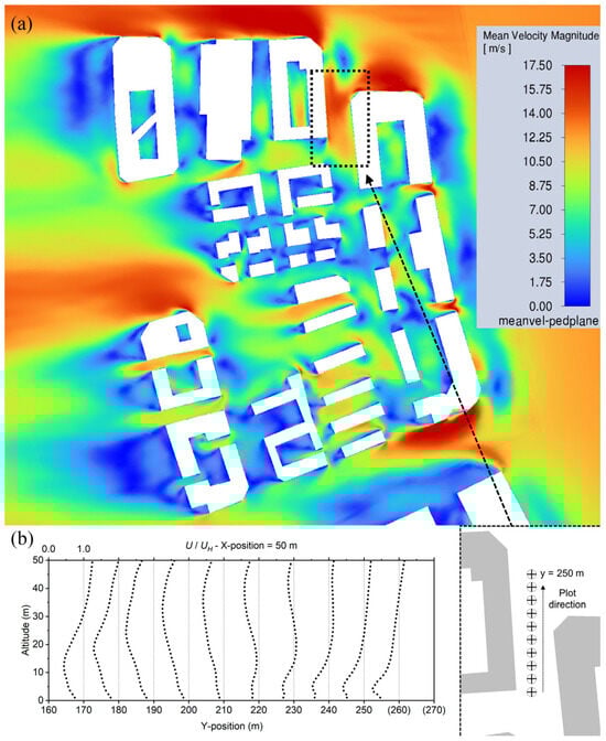
Figure 1.
(a) An example of spatial distribution of CFD-simulated time-averaged velocity at pedestrian level in a typical urban area of Shanghai. (b) The changes in the vertical profile for the selected area in (a).
2.2. Description of Urban Wind Resource
As described before, SWTs benefit from the local wind amplification brought by complex urban flow. However, the flow is not fixed, as magnitude and direction always change due to meteorological factors. An urban wind resource assessment, therefore, should consider the changing of weather conditions during a period of time, and as a result, CFD simulation must be performed with multiple and carefully designed conditions. Conditions should be designed with the following factors.
- (a)
- Wind direction and corresponding frequency;
- (b)
- Wind velocity and turbulence variables;
- (c)
- Extreme conditions considering natural windstorm disasters, especially tropical cyclones.
Acquiring the information with observation might be a difficulty, as a rigorous measurement period could be four years or more [23]. A common practice is to fit the short-period observation with a probability distribution and extrapolate the velocity with probability. The Weibull distribution is the most used one to represent the wind characteristics at a fixed location [24], even in the built environment [25]. The cumulative distribution function (CDF) and probability density function (PDF) of a three-parameter Weibull distribution is as in Equations (4) and (5) [26].
where x is the fitted variable, for example, the 10 min mean velocity magnitude of wind, and α, β, and ζ are parameters of the Weibull distribution. However, this fitting method can only shorten but not eliminate the observation process, and a small amount of observation data or other data of the same authenticity is always required. It is proven that the maximum likelihood estimation (MLE) is the most reliable and accurate method to fit the wind characteristics along a fixed period, in both unperturbed [27,28,29] and strongly perturbed urban [30,31] conditions. An MLE algorithm could be easily programmed and executed with any Python or MATLAB libraries accordingly.
With the Weibull distribution, it is also possible to acquire the accurate probability of extreme weather conditions that could be a challenge for the turbines. Typically, an extreme velocity value could be simply calculated by inversing Equation (4) and inputting the threshold probability, which is considered as the extreme.
2.3. Calculation of Energy Yield and Identification of Potential Wind Resource
The ultimate goal for urban wind resource assessment is to obtain the energy yield of SWTs at selected positions in the urban built environment. Therefore, it is crucial to understand the energy extraction process. An aerodynamic way to calculate the power of the wind (P) is described as Equation (6).
where ρ is the density of air, A is the swept area of the wind turbine, and U is the streamwise velocity of wind. However, wind turbines, in practice, can only harvest a small portion of the power of the wind, and the actual output power of the turbine is equal to the power of the wind multiplied by a power coefficient CP, as Equation (7) describes.
where PT is the output power of the turbine. The power coefficient CP is determined by the design and working condition of the turbine. A theoretical maximum of power coefficient CP is 59.3% and 29.6% for turbines using lifting force and drag force, respectively [32,33]. The power coefficient is typically drawn in a power curve, as a function against wind speed. The cut-in/out speeds define the domain of this function. Once the velocity of wind is beyond the domain, the power coefficient is zero.
It is obvious that a slight increase in wind speed can bring a significant increase in energy harvest, as the energy of the wind is linear to the cube of the velocity of wind. A good choice of installation position overshadows any technical advance in SWT itself.
Heterogeneous buildings in the urban area can create local amplifications of wind speed that are regarded as favorable to SWTs [34], and the typical flow patterns were revealed by different studies [35,36,37]. This review further categorizes those flow patterns into two types: detour flow and artificial venturi. Detour flows are the most common patterns, where the wind accelerates at the sides and top of a building. Artificial venturi usually appears on tall buildings that are specially designed for wind resource harnessing. These positions in an urban building cluster should be identified and considered as a sampling point in the related CFD simulation. Currently, the rooftops are the most investigated position for installing SWTs, where the amplification of wind due to detour can be fully utilized, and the spaces for installing SWTs are relatively larger. It was suggested to be feasible to gain more energy by installing both HAWTs [38] and VAWTs [39] on rooftops.
However, a larger wind speed often brings larger turbulence. Turbulence is usually described by turbulence intensity (I) or turbulent kinetic energy (k), and has a negative effect on SWTs’ output and lifespan [40]. Sometimes the overly high wind speed may lead to a cut-off as well. Therefore, a comprehensive wind resource assessment should consider the all of the performance parameters of an SWT.
3. CFD-Aided Assessment of Wind Resource
3.1. Handling of Turbulent Terms
CFD simulation is a numeric and approximate solution of the governing equations of the fluid dynamic based on finite volume method. These governing equations are the Navier–Stokes (N-S) equations, which satisfy the mass conservation and Newton’s second law. There are five major equations for a three-dimensional, confined and incompressible Newtonian flow, containing one continuity equation, three momentum equations, and one energy equation. For urban wind resource studies, the energy equation could be omitted because the Richardson number (Ri) is too low in the studied area, and the buoyancy effect cannot significantly affect the convective flow pattern. The N-S equations, however, are not solvable analytically, for there are partial-differential equation terms which describe the turbulent flow. Therefore, two major approaches were invented to turn convert these terms and solve the N-S equations numerically.
In the Reynolds-averaged Navier–Stokes (RANS) approach, the transient and turbulent flow is averaged in a temporal way, where the flow is regarded as steady and turbulence terms are modeled with steady parameters. Based on this approach, two different types of models were developed, namely the Boussinesq hypothesis-based models, including the Spalart–Allmaras (SA) model [41], k-ε series [42,43,44] and k-ω series [45] models, and the Reynolds stress transportation-based model, including the Reynolds Stress Model (RSM) [46]. For example, in the widely used k-ε and k-ω series models, the turbulent flow is averaged over flow time and modeled by turbulent kinetic energy (k) and its dissipation rate (ε) or specific dissipation rate (ω).
In the other widely adopted approach, large eddy simulation (LES), the flow is averaged spatially, where only large eddies are considered and the small eddies within the discretized cells are computed using sub-grid scale (SGS) models. For urban wind simulation, the Smagorinsky–Lily, wall-adapting local eddy-viscosity (WALE), and algebraic wall-modeled LES (WMLES) models are mostly used.
A figure from a previous review stunningly illustrated the difference between these two models [47], as Figure 2 shows. It should be noted that a direct Navier–Stokes (DNS) approach is not discussed here due to its infeasibility in application.
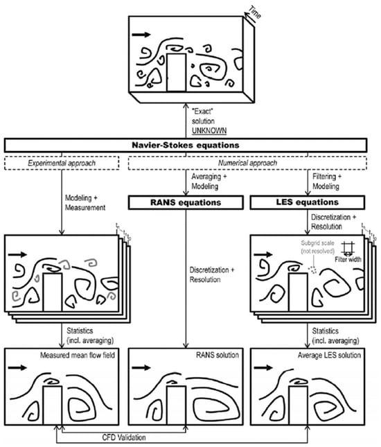
Figure 2.
RANS and LES models to simulate turbulent flows compared to reality [47].
A list of turbulence model utilization in relevant studies is shown in Table 1. It is clear that RANS models are being widely used to reconstruct the urban flow, while only a few studies selected LES models. The critical factor for selecting a turbulence model is the trade-off between simulation accuracy and computational cost, which are distinctly different between RANS and LES models.

Table 1.
Recent studies’ choices of turbulence models.
RANS models are known to acquire “a decent level of accuracy” with moderate computational cost. The most used k-ε series and k-ω series models solve only two more turbulence equations, while the RSM models must solve seven more equations in three-dimensional flow but give a more accurate solution. The one-equation SA model can of course acquire the solution with even less computational cost but with compromised accuracy. The common point of all RANS models is that their solution is acquired from a convergence process, which will consume a certain number of iterative time steps, and their result is steady and simple to process, with time-averaged velocity representing the momentum distribution within the domain, and turbulent variables representing the fluctuation of this momentum distribution. The LES and LES-based models can provide a transient solution that is closer to wind tunnel tests and on-site measurements, especially in predicting turbulence variables [72], but it requires a greater computational cost, at least one order higher than RANS models. LES only solves the flow within one time step in every iteration. Therefore, apart from its stringent requirement for a computational grid, which will be discussed in Section 3.2, the flow data will have to be collected through a long enough flow time, which further increases the computational cost.
In addition, the requirements of spatial discretization and temporal discretization are in fact coupled with a Courant–Friedrichs–Lewy (CFL) number requirement. This CFL number is defined as the flow characteristic velocity multiplied by the ratio of temporal discretization size to spatial discretization size, and is required to be less than 1.0 in non-iterative transient schemes [73]. Namely, the smaller the computational grid, a smaller time step size and a larger total flow time should be set. Here, a parameter denoting computational cost (CC) for a non-iterative transient scheme is defined in Equation (8).
where ccompute is a parameter depending on the researcher’s computing capacity, V and ΔV denote the volume of the whole computational domain and average grid cell, respectively, T and ΔT denote the flow time and average time step size, respectively, l denotes the average cell size, and uCFL is the characteristic velocity in CFL number. It is recommended that Tinit and Tsample are sufficient for the flow to have one and two complete flow-overs, respectively, in order to provide sampling-time-insensitive results. Equation (8) also suggests that, with a fixed CFL number and total flow time, computational cost is directly proportional to l−4 and will increase drastically with a refined computational grid. Consequently, LES models and LES-based hybrid models (including detached eddy simulation (DES) [74] and embedded LES (ELES)) are chosen less often to reconstruct urban flow, especially high-Re flows, as shown in Table 1.
The LES-based hybrid models, though rarely documented, could be a potential remedy for the high computational cost in urban wind engineering. Both DES and ELES models feature the reduction of the computation of resolved turbulence while keeping a good accuracy as pure LES modes. DES models treat the wall-bounded flow as modeled and the rest as resolved [75], while the ELES model treats the flow according to a manual partitioning of the computational domain. Studies have shown that DES and ELES models can both reach the same level of accuracy when predicting turbulent urban flows when tackling pedestrian-level wind comfort and wind hazard problems [76,77,78], building wind load and vibration problems [79,80], pollutant dispersion problems [81], and regular urban flow problems [82]. With all of these successful implementations in relevant studies, there is no reason that LES-based hybrid models should be excluded from the wind resource assessment toolbox. In practice, however, the accuracy of DES is dependent on finely tuned model constants and wall-bounded grids as well as the carefully chosen boundary layer RANS model to ensure a proper detaching position, and the grid count could be significantly reduced to save computational cost [77,82,83], up to 20% [76]. ELES in contrast, though accurate as well [78,80], can only mitigate the computational burden in the peripheral domain and may not be able to reduce the grid count to the same level as DES. Anyway, LES-based hybrid models are transient models, and will still suffer from the transient sampling process for a long enough period, guaranteeing the same order of magnitude for their computational cost as pure LES models.
Nevertheless, LES-based models provide a high-fidelity numerical method for computation wind engineering [84]. In particular, for a complex urban area, in most cases, the RANS simulation can hardly reconstruct the turbulence variables precisely and may underestimate the turbulent kinetic energy k or turbulence intensity (I) [47,85,86]. This drawback will adversely affect the estimation of lifespan [40] which is usually calculated from k or I. Thus, before choosing a turbulence model, researchers are recommended to fully consider their specific research demand and computing capacity. For instance, LES and LES-based hybrid models can provide detailed and dynamic results (e.g., in verification processes of an SWT’s installation), and RANS could be utilized on a large scale and with large design margins (e.g., in early-stages of wind resource assessment). Table 2 shows the performance of currently proven turbulence models for urban wind engineering.
Table 2.
Performance metrics of currently proven turbulence models.
Once the turbulence model is chosen, research should refer to the best practice guidelines (BPGs). There are many general BPGs on urban wind simulation and specific BPGs for pedestrian wind or building wind loads could also be referred to when conducting a computational wind engineering simulation. The COST BPG [87] published in 2004, which was based on the summarization of early CFD and wind-tunnel studies in Europe, is now recognized as the first conventional BPG on general wind engineering. This document was later updated in 2007 [88]. The Architectural Institute of Japan (AIJ) published their BPG on pedestrian wind as well as building wind load in 2008, concentrating on the CFD and wind-tunnel studies [18,89].
3.2. Computational Grid
A high-quality computational grid is fundamental to the computation convergence and accuracy of the results. The selection of grid type is determined by turbulence model, solution scheme, and grid independent analysis. When constructing the computational grid, it is recommended to roughly consider the following three points [18].
- (a)
- Distinguishing the core region from the peripheral region, and ensuring the cell sizes in the core region are one order smaller than local building size.
- (b)
- Refining the boundary layer region with cells parallel to the wall, and ensuring the expansion ratio is smaller than 1.5.
- (c)
- Generating three computational grids for validation purposes.
Once the grid is generated, it should be validated. The grid should be put into computation and results should be evaluated. The major indicator is the non-dimensional wall distance (y+), calculated using Equation (9).
where uτ is the friction velocity, y is the wall distance, ν is the kinematic viscosity, τw is the wall shear stress, and ρ is the density of the fluid. The local y+ value of a grid cell indicates its perpendicular position in the boundary layer.
Most RANS models have the wall-bounded flow modeled by wall functions (WFs). As a result, the y+ requirement is determined by the specific WF. In most cases, first-layer grid cells should fall in the logarithmic sublayer of the boundary layer. For example, when using a standard wall function for k-ε series models [90], the y+ of first layer grid cells should be between 30 and 100.
For LES studies, WFs are not applicable, and the wall-bounded flow should be resolved by the grid. In such cases, it is recognized that the y+ at all grid cells should be lower than or around 1.0 [91]; as a result, the first layer grid cells fall in the linear sublayer. In practice, however, some studies have shown the possibility of more flexible grid requirements, especially with LES models. For example, the velocity data sampled around the buildings is of high uniformity with different building y+ values, which range from 1.5 to 25 [92,93]. Some LES studies accepted even higher y+ values [11]. It should be emphasized that a y+ value beyond the model-specific range will definitely deteriorate the accuracy of the solution at the near-wall area, and whether this is acceptable in the context of the condition and interested area should be identified, as fully resolved wall-bounded flow is sometimes unnecessary and unpractical, especially for high-Re flows.
There is an additional requirement for LES grids, where they should be fine enough to resolve at least 80% of the total turbulent kinetic energy [94]. An LES_IQk is defined to signify this percentage as Equation (10) shows [95].
where k is the turbulent kinetic energy, h is the grid size, p is the order of accuracy of the numerical scheme, and ak is a coefficient to be determined by comparing the performance of two sets of computation grids. For urban wind resource assessment studies, it is critical to accurately reconstruct the velocity and turbulent variables at near-wall areas of urban buildings where the roof-mounted SWTs are installed. Therefore, a strict compliance of y+ and resolved turbulent kinetic energy requirement are strongly recommended for LES studies.
After the computational grid is validated with y+ and LES_IQk indicators, a grid independence analysis will be conducted. Velocity and turbulent variables are recommended for grid independence analysis, in line with other computational wind engineering studies. The power coefficient of the wind turbine could also be considered [70], as the error from different grids is not essential and will not hide the error with flow. There are two typical ways to report the grid independence. Most studies consider only a set of scatter or line plots in which points of solution from one grid against another are compared. The other way is to compute the grid convergence index (GCI), which is deduced from Richardson Extrapolation [96]. The GCI value is calculated using Equation (11).
where εr is the relative error of interested variables sampled at interested points, r is the size ratio of grids that exceeds 1.0, p is the discretization precision, and FS is the safety factor. A conservative value for FS is 3.0, but for practical application a moderate value of 1.25 could also be accepted [96]. The GCI values reported by previous studies were mostly under 5% [11,59,61,62,71].
3.3. Computational Domain and Boundary Conditions
The computational domain for a wind resource assessment study can follow the settings of existing computational wind engineering studies. The dimension of the computational domain should be large enough to prevent the venturi effect and contain the stagnation flow and wake [97]. The BPGs have defined the smallest domain size based on the size of the interested urban geometry [87,89]. It should be at least five times the height of the tallest building (5H) in the urban geometry for the upstream and side margins, 15H for the downstream margin, and 6H for the domain height. Studies from another perspective suggested that the domain should have a blockage ratio (a projected area of building façades against the inlet boundary area) smaller than 3% to contain all of the detour flows [18]. Following the BPGs [18,87], a CFD urban wind resource simulation should generally consider four types of boundaries as Table 3 shows.
Table 3.
Boundary conditions.
Boundary conditions in Table 3 are based on the recommended size of the computational domain. Special attention should be paid to the pairing of inlet and ground condition. The inlet ABL profile is determined by the terrain, and highly related to the ground roughness [98]. An ABL horizontal homogeneity check should always be performed in an empty domain, with same inlet and ground condition as the actual case, and the profile at the inlet plane and incident plane should be compared to confirm that the urban area is exposed to the correct inflow condition. There is no known study that deliberately implemented poorly-paired profiles to test their impact on building detour flow, which has a direct impact on SWT performance, but a relevant study on building wind load showed that a long upstream terrain (15H) without proper wall function will lead to error in the wind pressure coefficient up to 40% [99]. It is inferred that poorly-paired profiles will lead to errors in the simulated flow pattern and uncertainty in the final results of wind resource assessments.
Figure 3 shows the changes in the inlet profile with different ground roughness specifications [100]. The U and I denote the streamwise velocity and turbulence intensity, respectively, y0 denotes the aerodynamic roughness length, and KS denotes the physical or geometrical roughness height. However, in some cases where the upstream margin of the terrain is too large, even a correctly paired ground roughness specification is not capable of maintaining the ABL profile, signifying that the problem is with the model itself. For LES models, the only feasible remedy is to shorten the upstream margin as the boundary layer is fully resolved without a WF. For RANS models, the problem could be solved by replacing the standard WF with a modified one. For example, a modified, k-ε based WF is introduced to keep a perfect ABL homogeneity with less strict y+ requirements [101], and could be implanted in the solver with a user-defined function [99].
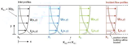
Figure 3.
ABL inhomogeneity [100].
In addition, the inlet condition for LES and LES-based hybrid models should be equipped with fully developed turbulence flow to ensure the incident profile is with fully developed turbulence. Numerous wind engineering studies have confirmed the superiority of the vortex method (VM) over other models [102], which stochastically generate the velocity fluctuation based on the input turbulence variable [93,103]. If an ELES model is used, this velocity fluctuation should be applied on the RANS-to-LES interface.
3.4. Validation of Authenticity
The validation process is primarily benchmarking the continuous and global data from CFD against the intermittent and local data from on-site measurement or the wind tunnel test. There are two types of validation, direct and indirect [104]. Direct validation is comparing the CFD results directly with observation results or experimental data. This type of validation is of high fidelity and can be applied only to the area of interest. However, direct validation for urban wind resources would require experimental data or observation results in the exact area of interest, which could be unpractical, as the desired condition in the real world cannot be reproduced. Indirect validation is essentially “model validation”, which validates only the CFD model under the same or a similar condition, and assumes the final results have the same fidelity as the ones in model validation. The former would always be preferred and recommended. However, for practical and specific studies, the latter would be used as measurement data are not always available.
For a wind resource assessment study, the validated variable should at least contain two core variables, namely the time-averaged velocity and turbulence intensity (or turbulent kinetic energy), in order to evaluate both the quantity and quality of wind energy. The final output of SWTs could also be considered if on-site measurement is available. For on-site measurement, light detection and ranging (LiDAR) [59,105,106,107] and an anemometer [108] are both capable of producing authentic data, while for the wind tunnel test, the most used is the hot-wire anemometer, which is in fact an invasive method and can only produce data with a lower level of reliability.
Once the data are obtained, a benchmarking should be conducted to compare the two datasets. Apart from benchmarking point by point [66], a comprehensive set of validation metrics is also utilized. For example, factor of two observations (FAC2) is defined to compare the data sampled at all points, as Equation (12) shows [109].
where
where P and Q are normalized CFD results and observations, and W is the threshold depending on the variable [88]. This validation indicator equals to one when CFD results are in good agreement with observations. Stricter validation indicators including FAC1.05 [110] and FAC1.3 [111] could be conducted by replacing 0.5 and 2 in Equation (13). Other validation indicators include hit rate (q), fractional bias (FB), and normalized mean square error (NMSE). Researchers are recommended to follow the exact quality acceptance criteria for each of the validation indicators [109] and compare the validation results with other relevant studies. For example, wind tunnel test data of a nine-block case could be a basis for benchmarking [112].
4. Challenges and Prospects
4.1. Limited Fidelity Brought by Turbulence Model
Through this review of CFD methods, several challenges are identified. These challenges limited the development of CFD-aided urban wind resource assessment.
As validated by multiple studies, LES and LES-based hybrid models are regarded as high-fidelity CFD models for urban flow [113,114]. However, as listed in Section 3.1, there is no sign of a significant increase in studies using LES and LES-based hybrid models. Witnessing the leap in computational capacity over the last few years, this review does not regard the high computational demand as the only reason for this lack of growth in the use of LES and LES-based hybrid models. As another review article pointed out, most BPGs in wind engineering are for RANS and there is a lack of BPGs for LES [104]. The lack of BPGs surely contributed to the limited use of LES models, which lowers the overall fidelity of this field of research. It should also be pointed out that this is even more serious for LES-based hybrid models. With validated accuracy and improved efficiency, these hybrid models should be utilized more widely, but they are not. As a result, recognized reviewers are appealed to for supplementing current BPGs and including these high-fidelity models.
Still, the choice of the turbulence model always depends on the scale and purpose of the study. High-fidelity models should be considered when assessing the wind resources on a building and community scale. Correspondingly, for assessing larger scales such as the overall wind resource of a whole city or town when larger computational resources are not available, RANS models should be considered as the feasible alternative.
4.2. Limited Fidelity Brought by Geometry Simplification
The fidelity of studies is also subject to the level of detail in building geometries. As Figure 4 depicts, in simplified geometries, the whole block is integrated into one object; in approximated geometries, the buildings are separately modeled; and in detailed geometries, the details including sloped rooftops are modeled. It is argued that an approximated building geometry provides a satisfactory degree of accuracy in the context of a wind profile above average building height [115]. However, the fine details on the rooftops cannot be neglected in wind resource assessment for SWTs. It is found that rooftop shapes can create a significant difference in detour flow above the building, with turbulent kinetic energy deviating up to 50% [9,116]. It is also found that even the slightest rounding of sharp edges of the rooftops can significantly change the shape of power density curves within the detour flow [48,117]. However, refining the geometry is only feasible in single-building studies or method studies. For large-scale simulation, using detailed geometry will cause a series of problems concerning the turbulence model and computational grid, as discussed in Section 3. Even if the turbulence model is specially tuned and validated to adapt those details, there is no source for such detailed building geometry, as the building geometry is normally extracted from GIS databases using a Shapefile format based on vectors [118]. A prospect for future studies is to quantitatively evaluate the deviation brought by geometry approximation, so the results for SWTs could be calculated from approximated building geometry and then calibrated by qualitative information on rooftops and façades.
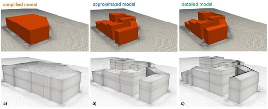
Figure 4.
Different building geometry detail levels, e.g., (a) simplified model; (b) approximated model; and (c) detailed model [115].
4.3. Wake Problems, Limitation of Benchmarking, and Extreme Conditions
An SWT can have 7.5 to 75 m2 of swept area, equivalent to a rotor diameter up to 10 m [33], which is close to the characteristic length scale of urban buildings. The wake of the turbine can create significant disturbance to urban flow pattern and generate strong turbulence for downstream SWTs, lowering the power generation and shortening the lifespan with increased fatigue [119]. Since a combined CFD simulation of SWTs and the building cluster is unpractical, turbines are never resolved in CFD simulations but modeled using wake models [120,121,122]. Studies have demonstrated the feasibility of applied wake models for HAWTs [38] and VAWTs [39,123] in the urban built environment. However, a lot of studies regarded the turbine wake as negligible and assessed the urban wind resource without an SWT wake model, leading to an overestimation in energy yield and underestimation of turbulence level.
From another perspective, a problem remains when wake models are applied on a large scale, where traditional wake models are still too complicated [124]. It is expected that future studies could apply parameterized models into the CFD wind assessment and realize the large-scale and wake-included simulations.
As mentioned in Section 2, extreme conditions considering natural windstorm disasters should be considered when carrying out a wind resource assessment. Studies have found that tropical cyclones, as a source of wind hazard, are increasing in frequency and intensity due to climate change [125,126]. Sadly, few studies discussed specifically the definition and simulation method of extreme conditions in wind resource assessment. Hence, future studies, when simulating the wind resources in the urban area, could also apply the extreme condition to the building cluster and acquire the extreme working condition of the SWTs. In addition, the urbanization around the globe is still ongoing [127], leading to changes in building morphology and corresponding boundary conditions for wind resource assessment.
4.4. Integration of Multi-Scale Modeling
Apart from the method-related challenges, the objects and focuses of those wind resource studies also provided insights for the potential evolution of CFD methods.
The urban environment and climate consist of different scales, including single facet, building, canyon and blocks, neighborhood, and city. The flow is affected by the forces across the range of different urban scales [21]. In most cases, the area of interest in wind resource assessment is surrounded by a dense urban area, which determines the local boundary condition and inlet profiles. The weather research and forecasting (WRF) model combined with the urban canopy model (UCM) is also a useful tool to provide authentic and local-scale (down to 1 × 1 km) conditions for the CFD simulation [128]. The weather research and forecasting (WRF) model could provide mesoscale velocity data with a resolution of 1 km and be converted into the format of a CFD inlet condition [129]. In fact, the inlet condition is of high complexity, and has to be considered together with wall functions (WFs). Usually, z0 follows the updated Davenport terrain classification [130], and the u* could be calculated from the given velocity at the given height. Studies have found that the coupled WRF-UCM performs better than conventional WRF in providing local-scale wind data [131,132].
4.5. Optimization Towards Application
The influencing factors of building-installed SWTs are relatively clear. A lot of studies discussed the effects of rooftop shape/angle [116,133], installation positions [53,134], and building layout/urban morphology [135]. Sadly, there is still a gap in practical application. Single building and idealized building arrays are repetitively investigated, the findings of which helped only local improvements such as rooftop shapes. Practical studies on a large scale and for real cities are, in contrast, seldom studied. A possible reason for this is the conflict between universality and particularity, in that many researchers might see a city-specific study as a multi-parameter problem, and its findings are too synthetic and case-specific to provide any insights for other scenarios.
Hence, this review sees two potential approaches towards a deeper understanding of factors affecting urban wind pattern and the distribution of urban wind resources. For idealized studies, multi-parameter optimization studies could be considered. These parameters include building geometry (height, height-width ratio, rooftop shape, etc.), turbine characteristics (turbine type, swept area, power curve, cut-in/out velocity, etc.), and conditions (wind rise, wind velocity distribution, upstream terrain roughness, etc.). The targets of this optimization include power, annual energy yield, and the lifespan of the SWT. In such studies, the computational cost for CFD simulation should be relatively low, and hundreds of cases could be performed with varying parameters, resulting in a quantitative and continuous understanding of what affects the SWT performance.
The other approach is to assess the wind resource of real cities and provide useful insight to the industry or policymakers, but that could raise the concern of high computational demand, as the largest scale for a pure CFD-based wind resource assessment is documented up to only 10 km [50] and cannot cover a modern megacity. Thus, it is promising that the CFD simulation could be combined with parameter analysis to realize the rapid reconstruction of the distribution of urban wind resources, as multiple studies have attempted for urban ventilation and wind comfort [136,137,138]. Data-driven methods could also be utilized to accelerate the reconstruction and optimization of urban flow based on CFD data [139]. Therefore, future studies on large-scale real cities will certainly deepen the understanding on urban flow and the application of urban SWTs.
5. Conclusions
This review systematically summarized the general process of a CFD-aided urban wind resource assessment for urban wind harnessing studies. Firstly, the conditions for urban wind resource assessment were addressed, including the extraction of boundary conditions and the performance of SWTs. Secondly, the commonly used CFD models are analyzed and provided with key points in configuration. It was found that LES, as a high-fidelity model, is still less used than the RANS model, which could be attributed to a lack of BPGs. However, LES-based hybrid models have not yet been used in urban wind resource assessment, and could offer a compromise as they balance the computational cost and accuracy. Thirdly, some challenges and corresponding prospects for future studies are discussed. These challenges include the fidelity problem of turbulence models and geometry simplification, the inclusion of wake models and extreme conditions, and larger scale application for real urban environments. At the same time, recent developments in multi-scale modeling and data-driven approaches show good potential for application, as they can be used in real city case modeling and accelerate the flow reconstruction and optimization. This review provides the technical basis for the CFD-aided urban wind simulation that can help to locate the starting point of such studies, and promote the application of state-of-the-art techniques in urban wind resource assessments.
Author Contributions
Conceptualization, R.C. and K.W.; writing—original draft preparation, R.C. and K.W.; writing—review and editing, R.C. and K.W.; supervision, K.W. All authors have read and agreed to the published version of the manuscript.
Funding
This research was supported by a SJTU start-up fund (WH220428004).
Data Availability Statement
Dataset available on request from the authors.
Conflicts of Interest
The authors declare no conflicts of interest.
Appendix A
Figure A1 shows the number of studies, as of 28 April 2025, that appeared in the search results for keywords mentioned in Section 1. The collection of studies shown here is not complete and is designed merely to demonstrate the increasing interest in CFD utilization in this field.
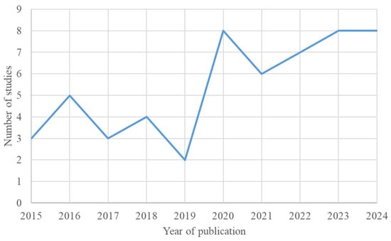
Figure A1.
Number of studies published from 2015 to 2024.
References
- IEA. Renewables 2024; IEA: Paris, France, 2024. [Google Scholar]
- Mobayen, S.; Assareh, E.; Izadyar, N.; Jamei, E.; Ahmadinejad, M.; Ghasemi, A.; Agarwal, S.; Pak, W. Multi-Functional Hybrid Energy System for Zero-Energy Residential Buildings: Integrating Hydrogen Production and Renewable Energy Solutions. Int. J. Hydrogen Energy 2025, 102, 647–672. [Google Scholar] [CrossRef]
- Bilgili, A.; Arda, T.; Kilic, B. Explainability in Wind Farm Planning: A Machine Learning Framework for Automatic Site Selection of Wind Farms. Energy Convers. Manag. 2024, 309, 118441. [Google Scholar] [CrossRef]
- Zhou, H.; Cao, Z.; Wang, Z.L.; Wu, Z. A Tightly Coupled Electromagnetic-Triboelectric Hybrid Generator for Wind Energy Harvesting and Environmental Monitoring. Nano Today 2025, 61, 102628. [Google Scholar] [CrossRef]
- Cooney, C.; Byrne, R.; Lyons, W.; O’Rourke, F. Performance Characterisation of a Commercial-Scale Wind Turbine Operating in an Urban Environment, Using Real Data. Energy Sustain. Dev. 2017, 36, 44–54. [Google Scholar] [CrossRef]
- Elagamy, M.; Tiwari, N.; Gallego-Castillo, C.; Cuerva-Tejero, A.; Lopez-Garcia, O.; Avila-Sanchez, S. Large Eddy Simulation of the Flow around a High-Rise Building with Special Focus on the Two-Points Two-Times Second Order Statistics of the Velocity Field. J. Wind Eng. Ind. Aerodyn. 2024, 254, 105914. [Google Scholar] [CrossRef]
- Prudden, S.; Fisher, A.; Marino, M.; Mohamed, A.; Watkins, S.; Wild, G. Measuring Wind with Small Unmanned Aircraft Systems. J. Wind Eng. Ind. Aerodyn. 2018, 176, 197–210. [Google Scholar] [CrossRef]
- Van Hooff, T.; Blocken, B. Full-Scale Measurements of Indoor Environmental Conditions and Natural Ventilation in a Large Semi-Enclosed Stadium: Possibilities and Limitations for CFD Validation. J. Wind Eng. Ind. Aerodyn. 2012, 104–106, 330–341. [Google Scholar] [CrossRef]
- Vranešević, K.K.; Vita, G.; Bordas, S.P.A.; Glumac, A.Š. Furthering Knowledge on the Flow Pattern around High-Rise Buildings: LES Investigation of the Wind Energy Potential. J. Wind Eng. Ind. Aerodyn. 2022, 226, 105029. [Google Scholar] [CrossRef]
- Stathopoulos, T.; Alrawashdeh, H.; Al-Quraan, A.; Blocken, B.; Dilimulati, A.; Paraschivoiu, M.; Pilay, P. Urban Wind Energy: Some Views on Potential and Challenges. J. Wind Eng. Ind. Aerodyn. 2018, 179, 146–157. [Google Scholar] [CrossRef]
- Juan, Y.-H.; Rezaeiha, A.; Montazeri, H.; Blocken, B.; Wen, C.-Y.; Yang, A.-S. CFD Assessment of Wind Energy Potential for Generic High-Rise Buildings in Close Proximity: Impact of Building Arrangement and Height. Appl. Energy 2022, 321, 119328. [Google Scholar] [CrossRef]
- Boikos, C.; Ioannidis, G.; Rapkos, N.; Tsegas, G.; Katsis, P.; Ntziachristos, L. Estimating Daily Road Traffic Pollution in Hong Kong Using CFD Modelling: Validation and Application. Build. Environ. 2025, 267, 112168. [Google Scholar] [CrossRef]
- Zou, J.; Yu, Y.; Mortezazadeh, M.; Lu, H.; Gaur, A.; Wang, L. Evaluating Climate Change Impacts on Building Level Steady-State and Dynamic Outdoor Thermal Comfort. Build. Environ. 2025, 271, 112604. [Google Scholar] [CrossRef]
- Santiago, J.L.; Martín, F.; Martilli, A. A Computational Fluid Dynamic Modelling Approach to Assess the Representativeness of Urban Monitoring Stations. Sci. Total Environ. 2013, 454–455, 61–72. [Google Scholar] [CrossRef]
- Toja-Silva, F.; Kono, T.; Peralta, C.; Lopez-Garcia, O.; Chen, J. A Review of Computational Fluid Dynamics (CFD) Simulations of the Wind Flow around Buildings for Urban Wind Energy Exploitation. J. Wind Eng. Ind. Aerodyn. 2018, 180, 66–87. [Google Scholar] [CrossRef]
- Vadhyar, A.; Sridhar, S.; Reshma, T.; Radhakrishnan, J. A Critical Assessment of the Factors Associated with the Implementation of Rooftop VAWTs: A Review. Energy Convers. Manag. X 2024, 22, 100563. [Google Scholar] [CrossRef]
- Richards, P.J. Appropriate Boundary Conditions for Computational Wind Engineering Models Using the K-E Turbulence Model. J. Wind. Eng. Ind. Aerodyn. 1974, 46–47, 145–153. [Google Scholar]
- Tominaga, Y.; Mochida, A.; Yoshie, R.; Kataoka, H.; Nozu, T.; Yoshikawa, M.; Shirasawa, T. AIJ Guidelines for Practical Applications of CFD to Pedestrian Wind Environment around Buildings. J. Wind Eng. Ind. Aerodyn. 2008, 96, 1749–1761. [Google Scholar] [CrossRef]
- Yang, Y.; Gu, M.; Chen, S.; Jin, X. New Inflow Boundary Conditions for Modelling the Neutral Equilibrium Atmospheric Boundary Layer in Computational Wind Engineering. J. Wind Eng. Ind. Aerodyn. 2009, 97, 88–95. [Google Scholar] [CrossRef]
- Richards, P.J.; Norris, S.E. Appropriate Boundary Conditions for Computational Wind Engineering Models Revisited. J. Wind Eng. Ind. Aerodyn. 2011, 99, 257–266. [Google Scholar] [CrossRef]
- Oke, T.R.; Mills, G.; Christen, A.; Voogt, J.A. Urban Climates; Cambridge University Press: Cambridge, UK, 2017. [Google Scholar]
- Barlow, J.F. Progress in Observing and Modelling the Urban Boundary Layer. Urban Clim. 2014, 10, 216–240. [Google Scholar] [CrossRef]
- Škvorc, P.; Kozmar, H. Wind Energy Harnessing on Tall Buildings in Urban Environments. Renew. Sustain. Energy Rev. 2021, 152, 111662. [Google Scholar] [CrossRef]
- Justus, C.G.; Hargraves, W.R.; Yalcin, A. Nationwide Assessment of Potential Output from Wind-Powered Generators. J. Appl. Meteorol. 1976, 15, 673–678. [Google Scholar] [CrossRef]
- Sunderland, K.; Woolmington, T.; Blackledge, J.; Conlon, M. Small Wind Turbines in Turbulent (Urban) Environments: A Consideration of Normal and Weibull Distributions for Power Prediction. J. Wind Eng. Ind. Aerodyn. 2013, 121, 70–81. [Google Scholar] [CrossRef]
- Weibull, W. A Statistical Distribution Function of Wide Applicability. J. Appl. Mech. 1951, 18, 293–297. [Google Scholar] [CrossRef]
- Bulut, A.; Bingöl, O. Weibull Parameter Estimation Methods on Wind Energy Applications—A Review of Recent Developments. Theor. Appl. Climatol. 2024, 155, 9157–9184. [Google Scholar] [CrossRef]
- Bingöl, F. Comparison of Weibull Estimation Methods for Diverse Winds. Adv. Meteorol. 2020, 2020, 3638423. [Google Scholar] [CrossRef]
- Carrillo, C.; Cidrás, J.; Díaz-Dorado, E.; Obando-Montaño, A. An Approach to Determine the Weibull Parameters for Wind Energy Analysis: The Case of Galicia (Spain). Energies 2014, 7, 2676–2700. [Google Scholar] [CrossRef]
- Wang, W.; Okaze, T. Statistical Analysis of Low-Occurrence Strong Wind Speeds at the Pedestrian Level around a Simplified Building Based on the Weibull Distribution. Build. Environ. 2022, 209, 108644. [Google Scholar] [CrossRef]
- Okaze, T.; Kikumoto, H.; Ono, H.; Imano, M.; Ikegaya, N.; Hasama, T.; Nakao, K.; Kishida, T.; Tabata, Y.; Nakajima, K.; et al. Large-Eddy Simulation of Flow around an Isolated Building: A Step-by-Step Analysis of Influencing Factors on Turbulent Statistics. Build. Environ. 2021, 202, 108021. [Google Scholar] [CrossRef]
- Mathew, S. Wind Energy; Springer: Berlin/Heidelberg, Germany, 2006; ISBN 978-3-540-30905-5. [Google Scholar]
- Hyams, M.A. Wind Energy in the Built Environment. In Metropolitan Sustainability; Elsevier: Amsterdam, The Netherlands, 2012; pp. 457–499. ISBN 978-0-85709-046-1. [Google Scholar]
- Dai, Y.; Tu, W.; Zhang, X.; Li, J.; Yue, X.; Wang, H. Dynamic Wind Patterns and Indoor/Outdoor Pollutant Dispersion in the Simplified Building Array: Statistical and Spectral Analyses from Scaled Outdoor Experiments. Build. Environ. 2025, 276, 112861. [Google Scholar] [CrossRef]
- Liu, S.; Zhang, L.; Lu, J.; Zhang, X.; Wang, K.; Gan, Z.; Liu, X.; Jing, Z.; Cui, X.; Wang, H. Advances in Urban Wind Resource Development and Wind Energy Harvesters. Renew. Sustain. Energy Rev. 2025, 207, 114943. [Google Scholar] [CrossRef]
- Micallef, D.; Van Bussel, G. A Review of Urban Wind Energy Research: Aerodynamics and Other Challenges. Energies 2018, 11, 2204. [Google Scholar] [CrossRef]
- Park, J.; Jung, H.-J.; Lee, S.-W.; Park, J. A New Building-Integrated Wind Turbine System Utilizing the Building. Energies 2015, 8, 11846–11870. [Google Scholar] [CrossRef]
- Zhang, S.; Du, B.; Ge, M.; Zuo, Y. Study on the Operation of Small Rooftop Wind Turbines and Its Effect on the Wind Environment in Blocks. Renew. Energy 2022, 183, 708–718. [Google Scholar] [CrossRef]
- Balduzzi, F.; Bianchini, A.; Carnevale, E.A.; Ferrari, L.; Magnani, S. Feasibility Analysis of a Darrieus Vertical-Axis Wind Turbine Installation in the Rooftop of a Building. Appl. Energy 2012, 97, 921–929. [Google Scholar] [CrossRef]
- Allen, S.R.; Hammond, G.P.; McManus, M.C. Energy Analysis and Environmental Life Cycle Assessment of a Micro-Wind Turbine. Proc. Inst. Mech. Eng. A J. Power Energy 2008, 222, 669–684. [Google Scholar] [CrossRef]
- Spalart, P.; Allmaras, S. A One-Equation Turbulence Model for Aerodynamic Flows. In Proceedings of the 30th Aerospace Sciences Meeting and Exhibit, Reno, NV, USA, 6–9 January 1992; American Institute of Aeronautics and Astronautics: Reston, VG, USA, 1992. [Google Scholar]
- Jones, W.P.; Launder, B.E. The Prediction of Laminarization with a Two-Equation Model of Turbulence. Int. J. Heat Mass Transfer. 1972, 15, 301–314. [Google Scholar] [CrossRef]
- Shih, T.-H.; Liou, W.W.; Shabbir, A.; Yang, Z.; Zhu, J. A New K-ϵ Eddy Viscosity Model for High Reynolds Number Turbulent Flows. Comput. Fluids 1995, 24, 227–238. [Google Scholar] [CrossRef]
- Yakhot, V.; Orszag, S.A. Renormalization Group Analysis of Turbulence. I. Basic Theory. J. Sci. Comput. 1986, 1, 3–51. [Google Scholar] [CrossRef]
- Launder, B.E. Turbulence Modelling for CFD. J. Fluid Mech. 1995, 289, 406–407. [Google Scholar] [CrossRef]
- Launder, B.E.; Reece, G.J.; Rodi, W. Progress in the Development of a Reynolds-Stress Turbulence Closure. J. Fluid Mech. 1975, 68, 537–566. [Google Scholar] [CrossRef]
- Blocken, B. LES over RANS in Building Simulation for Outdoor and Indoor Applications: A Foregone Conclusion? Build. Simul. 2018, 11, 821–870. [Google Scholar] [CrossRef]
- Zanforlin, S.; Letizia, S. Improving the Performance of Wind Turbines in Urban Environment by Integrating the Action of a Diffuser with the Aerodynamics of the Rooftops. Energy Procedia 2015, 82, 774–781. [Google Scholar] [CrossRef]
- Wang, B.; Cot, L.D.; Adolphe, L.; Geoffroy, S.; Morchain, J. Estimation of Wind Energy over Roof of Two Perpendicular Buildings. Energy Build. 2015, 88, 57–67. [Google Scholar] [CrossRef]
- Simões, T.; Estanqueiro, A. A New Methodology for Urban Wind Resource Assessment. Renew. Energy 2016, 89, 598–605. [Google Scholar] [CrossRef]
- Kono, T.; Kogaki, T.; Kiwata, T. Numerical Investigation of Wind Conditions for Roof-Mounted Wind Turbines: Effects of Wind Direction and Horizontal Aspect Ratio of a High-Rise Cuboid Building. Energies 2016, 9, 907. [Google Scholar] [CrossRef]
- Krishnan, A.; Paraschivoiu, M. 3D Analysis of Building Mounted VAWT with Diffuser Shaped Shroud. Sustain. Cities Soc. 2016, 27, 160–166. [Google Scholar] [CrossRef]
- Larin, P.; Paraschivoiu, M.; Aygun, C. CFD Based Synergistic Analysis of Wind Turbines for Roof Mounted Integration. J. Wind Eng. Ind. Aerodyn. 2016, 156, 1–13. [Google Scholar] [CrossRef]
- Zhou, H.; Lu, Y.; Liu, X.; Chang, R.; Wang, B. Harvesting Wind Energy in Low-Rise Residential Buildings: Design and Optimization of Building Forms. J. Clean. Prod. 2017, 167, 306–316. [Google Scholar] [CrossRef]
- Abohela, I.; Hamza, N.; Dudek, S. Effect of Roof Shape, Wind Direction, Building Height and Urban Configuration on the Energy Yield and Positioning of Roof Mounted Wind Turbines. Renew. Energy 2013, 50, 1106–1118. [Google Scholar] [CrossRef]
- Aquino, A.I.; Calautit, J.K.; Hughes, B.R. Integration of Aero-Elastic Belt into the Built Environment for Low-Energy Wind Harnessing: Current Status and a Case Study. Energy Convers. Manag. 2017, 149, 830–850. [Google Scholar] [CrossRef]
- Hassanli, S.; Hu, G.; Kwok, K.C.S.; Fletcher, D.F. Utilizing Cavity Flow within Double Skin Façade for Wind Energy Harvesting in Buildings. J. Wind Eng. Ind. Aerodyn. 2017, 167, 114–127. [Google Scholar] [CrossRef]
- Liu, S.; Pan, W.; Zhang, H.; Cheng, X.; Long, Z.; Chen, Q. CFD Simulations of Wind Distribution in an Urban Community with a Full-Scale Geometrical Model. Build. Environ. 2017, 117, 11–23. [Google Scholar] [CrossRef]
- Wang, Q.; Wang, J.; Hou, Y.; Yuan, R.; Luo, K.; Fan, J. Micrositing of Roof Mounting Wind Turbine in Urban Environment: CFD Simulations and Lidar Measurements. Renew. Energy 2018, 115, 1118–1133. [Google Scholar] [CrossRef]
- Zabarjad Shiraz, M.; Dilimulati, A.; Paraschivoiu, M. Wind Power Potential Assessment of Roof Mounted Wind Turbines in Cities. Sustain. Cities Soc. 2020, 53, 101905. [Google Scholar] [CrossRef]
- Longo, R.; Nicastro, P.; Natalini, M.; Schito, P.; Mereu, R.; Parente, A. Impact of Urban Environment on Savonius Wind Turbine Performance: A Numerical Perspective. Renew. Energy 2020, 156, 407–422. [Google Scholar] [CrossRef]
- Alanis Ruiz, C.; Kalkman, I.; Blocken, B. Aerodynamic Design Optimization of Ducted Openings through High-Rise Buildings for Wind Energy Harvesting. Build. Environ. 2021, 202, 108028. [Google Scholar] [CrossRef]
- Fan, X.; Ge, M.; Tan, W.; Li, Q. Impacts of Coexisting Buildings and Trees on the Performance of Rooftop Wind Turbines: An Idealized Numerical Study. Renew. Energy 2021, 177, 164–180. [Google Scholar] [CrossRef]
- Juan, Y.-H.; Wen, C.-Y.; Li, Z.; Yang, A.-S. Impacts of Urban Morphology on Improving Urban Wind Energy Potential for Generic High-Rise Building Arrays. Appl. Energy 2021, 299, 117304. [Google Scholar] [CrossRef]
- Dai, S.F.; Liu, H.J.; Peng, H.Y. Assessment of Parapet Effect on Wind Flow Properties and Wind Energy Potential over Roofs of Tall Buildings. Renew. Energy 2022, 199, 826–839. [Google Scholar] [CrossRef]
- Mi, L.; Han, Y.; Shen, L.; Cai, C.; Wu, T. Multi-Scale Numerical Assessments of Urban Wind Resource Using Coupled WRF-BEP and RANS Simulation: A Case Study. Atmosphere 2022, 13, 1753. [Google Scholar] [CrossRef]
- Paula, C.; José, C.; Leorlen, M.; Daniel, G.; Alexandre, C.; Teresa, S. Wind Resource Assessment in Building Environment: Benchmarking of Numerical Approaches and Validation with Wind Tunnel Data. Wind 2022, 2, 659–690. [Google Scholar] [CrossRef]
- Dai, S.F.; Liu, H.J.; Chu, Y.J.; Lam, H.F.; Peng, H.Y. Impact of Corner Modification on Wind Characteristics and Wind Energy Potential over Flat Roofs of Tall Buildings. Energy 2022, 241, 122920. [Google Scholar] [CrossRef]
- Tominaga, Y. CFD Prediction for Wind Power Generation by a Small Vertical Axis Wind Turbine: A Case Study for a University Campus. Energies 2023, 16, 4912. [Google Scholar] [CrossRef]
- Rezaei, F.; Paraschivoiu, M. Computational Study of the Effect of Building Height on the Performance of Roof-Mounted VAWT. J. Wind Eng. Ind. Aerodyn. 2023, 241, 105540. [Google Scholar] [CrossRef]
- Juan, Y.-H.; Rezaeiha, A.; Montazeri, H.; Blocken, B.; Yang, A.-S. Improvement of Wind Energy Potential through Building Corner Modifications in Compact Urban Areas. J. Wind Eng. Ind. Aerodyn. 2024, 248, 105710. [Google Scholar] [CrossRef]
- Shirzadi, M.; Tominaga, Y. CFD Evaluation of Mean and Turbulent Wind Characteristics around a High-Rise Building Affected by Its Surroundings. Build. Environ. 2022, 225, 109637. [Google Scholar] [CrossRef]
- Courant, R.; Friedrichs, K.; Lewy, H. On the Partial Difference Equations of Mathematical Physics. IBM J. Res. Dev. 1967, 11, 215–234. [Google Scholar] [CrossRef]
- Spalart, P.R. Comments on the Feasibility of LES for Wings, and on a Hybrid RANS/LES Approach. In Proceedings of the First AFOSR International Conference on DNS/LES, Ruston, LA, USA, 4–8 August 1997. [Google Scholar]
- Spalart, P.R. Detached-Eddy Simulation. Annu. Rev. Fluid Mech. 2009, 41, 181–202. [Google Scholar] [CrossRef]
- Liu, J.; Niu, J. Delayed Detached Eddy Simulation of Pedestrian-Level Wind around a Building Array—The Potential to Save Computing Resources. Build. Environ. 2019, 152, 28–38. [Google Scholar] [CrossRef]
- Liu, J.; Niu, J.; Mak, C.M.; Xia, Q. Detached Eddy Simulation of Pedestrian-Level Wind and Gust around an Elevated Building. Build. Environ. 2017, 125, 168–179. [Google Scholar] [CrossRef]
- Zhang, Y.; Cao, S.; Cao, J. A Framework for Efficient Simulation of Urban Strong Wind Field during Typhoon Process Using Coupled WRF-UCM and Embedded LES Model. J. Wind Eng. Ind. Aerodyn. 2024, 250, 105757. [Google Scholar] [CrossRef]
- Zhang, Y.; Habashi, W.G.; Khurram, R.A. Predicting Wind-Induced Vibrations of High-Rise Buildings Using Unsteady CFD and Modal Analysis. J. Wind Eng. Ind. Aerodyn. 2015, 136, 165–179. [Google Scholar] [CrossRef]
- Zhang, Y.; Cao, S.; Cao, J. Implementation of an Embedded LES Model with Parameter Assessment for Predicting Surface Pressure and Surrounding Flow of an Isolated Building. Build. Environ. 2023, 243, 110633. [Google Scholar] [CrossRef]
- Wang, X.; Lei, H.; Han, Z.; Zhou, D.; Shen, Z.; Zhang, H.; Zhu, H.; Bao, Y. Three-Dimensional Delayed Detached-Eddy Simulation of Wind Flow and Particle Dispersion in the Urban Environment. Atmos. Environ. 2019, 201, 173–189. [Google Scholar] [CrossRef]
- Sharma, A.; Mittal, H.; Gairola, A. Detached-Eddy Simulation of Interference between Buildings in Tandem Arrangement. J. Build. Eng. 2019, 21, 129–140. [Google Scholar] [CrossRef]
- Dadioti, R.; Rees, S. Performance of Detached Eddy Simulation Applied to Analysis of a University Campus Wind Environment. Energy Procedia 2017, 134, 366–375. [Google Scholar] [CrossRef]
- Tominaga, Y.; Mochida, A.; Murakami, S.; Sawaki, S. Comparison of Various Revised k–ε Models and LES Applied to Flow around a High-Rise Building Model with 1:1:2 Shape Placed within the Surface Boundary Layer. J. Wind Eng. Ind. Aerodyn. 2008, 96, 389–411. [Google Scholar] [CrossRef]
- Blocken, B. 50 Years of Computational Wind Engineering: Past, Present and Future. J. Wind Eng. Ind. Aerodyn. 2014, 129, 69–102. [Google Scholar] [CrossRef]
- Van Hooff, T.; Blocken, B.; Tominaga, Y. On the Accuracy of CFD Simulations of Cross-Ventilation Flows for a Generic Isolated Building: Comparison of RANS, LES and Experiments. Build. Environ. 2017, 114, 148–165. [Google Scholar] [CrossRef]
- Franke, J.; Hirsch, C.; Jensen, A.G.; Krüs, H.W.; Schatzmann, M.; Westbury, P.S.; Miles, S.D.; Wisse, J.A.; Wright, N.G. Recommendations on the Use of CFD in Wind Engineering. 2004. Available online: http://ftp.demec.ufpr.br/CFD/bibliografia/erros_numericos/Franke_et_al_sem-data.pdf (accessed on 1 April 2025).
- Franke, J.; Hellsten, A.; Schlunzen, K.H.; Carissimo, B. The COST 732 Best Practice Guideline for CFD Simulation of Flows in the Urban Environment: A Summary. Int. J. Environ. Pollut. 2011, 44, 419. [Google Scholar] [CrossRef]
- Tamura, T.; Nozawa, K.; Kondo, K. AIJ Guide for Numerical Prediction of Wind Loads on Buildings. J. Wind Eng. Ind. Aerodyn. 2008, 96, 1974–1984. [Google Scholar] [CrossRef]
- Launder, B.E.; Spalding, D.B. The Numerical Computation of Turbulent Flows. Comput. Methods Appl. Mech. Eng. 1974, 3, 269–289. [Google Scholar] [CrossRef]
- Georgiadis, N.J.; Rizzetta, D.P.; Fureby, C. Large-Eddy Simulation: Current Capabilities, Recommended Practices, and Future Research. AIAA J. 2010, 48, 1772–1784. [Google Scholar] [CrossRef]
- Liu, J.; Niu, J.; Du, Y.; Mak, C.M.; Zhang, Y. LES for Pedestrian Level Wind around an Idealized Building Array—Assessment of Sensitivity to Influencing Parameters. Sustain. Cities Soc. 2019, 44, 406–415. [Google Scholar] [CrossRef]
- Ai, Z.T.; Mak, C.M. Large-Eddy Simulation of Flow and Dispersion around an Isolated Building: Analysis of Influencing Factors. Comput. Fluids 2015, 118, 89–100. [Google Scholar] [CrossRef]
- Pope, S.B. Turbulent Flows; 1. publ., 12. print.; Cambridge University Press: Cambridge, UK, 2015; ISBN 978-0-521-59886-6. [Google Scholar]
- Celik, I.B.; Cehreli, Z.N.; Yavuz, I. Index of Resolution Quality for Large Eddy Simulations. J. Fluids Eng. 2005, 127, 949–958. [Google Scholar] [CrossRef]
- Roache, P.J. Quantification of Uncertainty in Computational Fluid Dynamics. Annu. Rev. Fluid Mech. 1997, 29, 123–160. [Google Scholar] [CrossRef]
- Blocken, B. Computational Fluid Dynamics for Urban Physics: Importance, Scales, Possibilities, Limitations and Ten Tips and Tricks towards Accurate and Reliable Simulations. Build. Environ. 2015, 91, 219–245. [Google Scholar] [CrossRef]
- Ricci, A.; Burlando, M.; Repetto, M.P.; Blocken, B. Simulation of Urban Boundary and Canopy Layer Flows in Port Areas Induced by Different Marine Boundary Layer Inflow Conditions. Sci. Total Environ. 2019, 670, 876–892. [Google Scholar] [CrossRef]
- Abu-Zidan, Y.; Mendis, P.; Gunawardena, T. Impact of Atmospheric Boundary Layer Inhomogeneity in CFD Simulations of Tall Buildings. Heliyon 2020, 6, e04274. [Google Scholar] [CrossRef] [PubMed]
- Blocken, B.; Carmeliet, J.; Stathopoulos, T. CFD Evaluation of Wind Speed Conditions in Passages between Parallel Buildings—Effect of Wall-Function Roughness Modifications for the Atmospheric Boundary Layer Flow. J. Wind Eng. Ind. Aerodyn. 2007, 95, 941–962. [Google Scholar] [CrossRef]
- Parente, A.; Benocci, C. On the RANS Simulation of Neutral ABL Flows. In Proceedings of the Fifth International Symposium on Computational Wind Engineering, Chapel Hill, NC, USA, 23–27 May 2010. [Google Scholar]
- Mathey, F.; Cokljat, D.; Bertoglio, J.P.; Sergent, E. Assessment of the Vortex Method for Large Eddy Simulation Inlet Conditions. Prog. Comput. Fluid Dyn. Int. J. 2006, 6, 58. [Google Scholar] [CrossRef]
- Gousseau, P.; Blocken, B.; Van Heijst, G.J.F. Quality Assessment of Large-Eddy Simulation of Wind Flow around a High-Rise Building: Validation and Solution Verification. Comput. Fluids 2013, 79, 120–133. [Google Scholar] [CrossRef]
- Tominaga, Y.; Wang, L.; Zhai, Z.; Stathopoulos, T. Accuracy of CFD Simulations in Urban Aerodynamics and Microclimate: Progress and Challenges. Build. Environ. 2023, 243, 110723. [Google Scholar] [CrossRef]
- Karthikeya, B.R.; Negi, P.S.; Srikanth, N. Wind Resource Assessment for Urban Renewable Energy Application in Singapore. Renew. Energy 2016, 87, 403–414. [Google Scholar] [CrossRef]
- Meteorological and Air Quality Models for Urban Areas; Baklanov, A., Sue, G., Alexander, M., Athanassiadou, M., Eds.; Springer: Berlin/Heidelberg, Germany, 2009; ISBN 978-3-642-00297-7. [Google Scholar]
- Lane, S.E.; Barlow, J.F.; Wood, C.R. An Assessment of a Three-Beam Doppler Lidar Wind Profiling Method for Use in Urban Areas. J. Wind Eng. Ind. Aerodyn. 2013, 119, 53–59. [Google Scholar] [CrossRef]
- Song, M.X.; Chen, K.; He, Z.Y.; Zhang, X. Wind Resource Assessment on Complex Terrain Based on Observations of a Single Anemometer. J. Wind Eng. Ind. Aerodyn. 2014, 125, 22–29. [Google Scholar] [CrossRef]
- Schatzmann, M.; Olesen, H.; Franke, J. Cost 732 Model Evaluation Case Studies: Approach and Results; COST Office: Brussels, Belgium, 2010. [Google Scholar]
- Iousef, S.; Montazeri, H.; Blocken, B.; Van Wesemael, P.J.V. On the Use of Non-Conformal Grids for Economic LES of Wind Flow and Convective Heat Transfer for a Wall-Mounted Cube. Build. Environ. 2017, 119, 44–61. [Google Scholar] [CrossRef]
- Ricci, A.; Kalkman, I.; Blocken, B.; Burlando, M.; Repetto, M.P. Impact of Turbulence Models and Roughness Height in 3D Steady RANS Simulations of Wind Flow in an Urban Environment. Build. Environ. 2020, 171, 106617. [Google Scholar] [CrossRef]
- Tominaga, Y.; Shirzadi, M. Wind Tunnel Measurement Dataset of 3D Turbulent Flow around a Group of Generic Buildings with and without a High-Rise Building. Data Brief 2021, 39, 107504. [Google Scholar] [CrossRef] [PubMed]
- Shaukat, U.; Jakobsen, J.B.; Ikegaya, N.; Giljarhus, K.E.T. Validation of Large Eddy Simulations in Urban Wind Studies Using a New Overall Area Metric. Build. Environ. 2025, 267, 112285. [Google Scholar] [CrossRef]
- Yan, Z.; Chen, R.; Cai, X.-C. Large Eddy Simulation of the Wind Flow in a Realistic Full-Scale Urban Community with a Scalable Parallel Algorithm. Comput. Phys. Commun. 2022, 270, 108170. [Google Scholar] [CrossRef]
- Ricci, A.; Kalkman, I.; Blocken, B.; Burlando, M.; Freda, A.; Repetto, M.P. Local-Scale Forcing Effects on Wind Flows in an Urban Environment: Impact of Geometrical Simplifications. J. Wind Eng. Ind. Aerodyn. 2017, 170, 238–255. [Google Scholar] [CrossRef]
- Toja-Silva, F.; Peralta, C.; Lopez-Garcia, O.; Navarro, J.; Cruz, I. On Roof Geometry for Urban Wind Energy Exploitation in High-Rise Buildings. Computation 2015, 3, 299–325. [Google Scholar] [CrossRef]
- Yang, A.-S.; Su, Y.-M.; Wen, C.-Y.; Juan, Y.-H.; Wang, W.-S.; Cheng, C.-H. Estimation of Wind Power Generation in Dense Urban Area. Appl. Energy 2016, 171, 213–230. [Google Scholar] [CrossRef]
- Wang, C.; Ferrando, M.; Causone, F.; Jin, X.; Zhou, X.; Shi, X. Data Acquisition for Urban Building Energy Modeling: A Review. Build. Environ. 2022, 217, 109056. [Google Scholar] [CrossRef]
- Vermeer, L.J.; Sørensen, J.N.; Crespo, A. Wind Turbine Wake Aerodynamics. Prog. Aerosp. Sci. 2003, 39, 467–510. [Google Scholar] [CrossRef]
- Sanderse, B. Aerodynamics of Wind Turbine Wakes Literature Review; Energy Research Centre of the Netherlands (ECN): Petten, The Netherlands, 2009. [Google Scholar]
- Sedaghatizadeh, N.; Arjomandi, M.; Kelso, R.; Cazzolato, B.; Ghayesh, M.H. Modelling of Wind Turbine Wake Using Large Eddy Simulation. Renew. Energy 2018, 115, 1166–1176. [Google Scholar] [CrossRef]
- Li, Z.; Yang, X. Evaluation of Actuator Disk Model Relative to Actuator Surface Model for Predicting Utility-Scale Wind Turbine Wakes. Energies 2020, 13, 3574. [Google Scholar] [CrossRef]
- Li, G.; Li, Y.; Li, J.; Huang, H.; Huang, L. Research on Dynamic Characteristics of Vertical Axis Wind Turbine Extended to the Outside of Buildings. Energy 2023, 272, 127182. [Google Scholar] [CrossRef]
- Li, Z.; Liu, X.; Yang, X. Review of Turbine Parameterization Models for Large-Eddy Simulation of Wind Turbine Wakes. Energies 2022, 15, 6533. [Google Scholar] [CrossRef]
- Emanuel, K. Increasing Destructiveness of Tropical Cyclones over the Past 30 Years. Nature 2005, 436, 686–688. [Google Scholar] [CrossRef] [PubMed]
- Bhatia, K.; Vecchi, G.; Murakami, H.; Underwood, S.; Kossin, J. Projected Response of Tropical Cyclone Intensity and Intensification in a Global Climate Model. J. Clim. 2018, 31, 8281–8303. [Google Scholar] [CrossRef]
- Zhang, D.; Xu, J.; Zhang, Y.; Wang, J.; He, S.; Zhou, X. Study on Sustainable Urbanization Literature Based on Web of Science, Scopus, and China National Knowledge Infrastructure: A Scientometric Analysis in CiteSpace. J. Clean. Prod. 2020, 264, 121537. [Google Scholar] [CrossRef]
- Bandoc, G.; Prăvălie, R.; Patriche, C.; Degeratu, M. Spatial Assessment of Wind Power Potential at Global Scale. A Geographical Approach. J. Clean. Prod. 2018, 200, 1065–1086. [Google Scholar] [CrossRef]
- Castorrini, A.; Gentile, S.; Geraldi, E.; Bonfiglioli, A. Investigations on Offshore Wind Turbine Inflow Modelling Using Numerical Weather Prediction Coupled with Local-Scale Computational Fluid Dynamics. Renew. Sustain. Energy Rev. 2023, 171, 113008. [Google Scholar] [CrossRef]
- Wieringa, J. Updating the Davenport Roughness Classification; IQPC: New York, NY, USA, 1992. [Google Scholar]
- He, X.; Li, Y.; Wang, X.; Chen, L.; Yu, B.; Zhang, Y.; Miao, S. High-Resolution Dataset of Urban Canopy Parameters for Beijing and Its Application to the Integrated WRF/Urban Modelling System. J. Clean. Prod. 2019, 208, 373–383. [Google Scholar] [CrossRef]
- Khan, A.; Chatterjee, S.; Weng, Y. Context and Background of Urban Heat Island. In Urban Heat Island Modeling for Tropical Climates; Elsevier: Amsterdam, The Netherlands, 2021; pp. 1–35. ISBN 978-0-12-819669-4. [Google Scholar]
- Toja-Silva, F.; Lopez-Garcia, O.; Peralta, C.; Navarro, J.; Cruz, I. An Empirical–Heuristic Optimization of the Building-Roof Geometry for Urban Wind Energy Exploitation on High-Rise Buildings. Appl. Energy 2016, 164, 769–794. [Google Scholar] [CrossRef]
- Ledo, L.; Kosasih, P.B.; Cooper, P. Roof Mounting Site Analysis for Micro-Wind Turbines. Renew. Energy 2011, 36, 1379–1391. [Google Scholar] [CrossRef]
- Lu, L.; Ip, K.Y. Investigation on the Feasibility and Enhancement Methods of Wind Power Utilization in High-Rise Buildings of Hong Kong. Renew. Sustain. Energy Rev. 2009, 13, 450–461. [Google Scholar] [CrossRef]
- Lim, J.; Ooka, R.; Lim, H. Multicollinearity Issue for the Parameterization of Urban Ventilation Potential with Urban Morphology. Sustain. Cities Soc. 2022, 87, 104218. [Google Scholar] [CrossRef]
- Li, J.; You, W.; Peng, Y.; Ding, W. Exploring the Potential of the Aspect Ratio to Predict Flow Patterns in Actual Urban Spaces for Ventilation Design by Comparing the Idealized and Actual Canyons. Sustain. Cities Soc. 2024, 102, 105214. [Google Scholar] [CrossRef]
- Li, Z.; Han, B.; Chu, Y.; Shi, Y.; Huang, N.; Shi, T. Evaluating the Impact of Road Layout Patterns on Pedestrian-Level Ventilation Using Computational Fluid Dynamics (CFD). Atmosphere 2025, 16, 123. [Google Scholar] [CrossRef]
- Shao, X.; Liu, Z.; Zhang, S.; Zhao, Z.; Hu, C. PIGNN-CFD: A Physics-Informed Graph Neural Network for Rapid Predicting Urban Wind Field Defined on Unstructured Mesh. Build. Environ. 2023, 232, 110056. [Google Scholar] [CrossRef]
Disclaimer/Publisher’s Note: The statements, opinions and data contained in all publications are solely those of the individual author(s) and contributor(s) and not of MDPI and/or the editor(s). MDPI and/or the editor(s) disclaim responsibility for any injury to people or property resulting from any ideas, methods, instructions or products referred to in the content. |
© 2025 by the authors. Licensee MDPI, Basel, Switzerland. This article is an open access article distributed under the terms and conditions of the Creative Commons Attribution (CC BY) license (https://creativecommons.org/licenses/by/4.0/).