Abstract
Urban Building Energy Modelling (UBEM) represents a comprehensive approach to investigate the intricate interplay of the various factors impacting energy use of groups of buildings, offering invaluable insights for urban planners, architects, building engineers, and policymakers. Nonetheless, available UBEM tools are still “research tools” and lack a unified standard addressing input, output, nomenclature, and calculation approaches. In this context, this study aims to conduct a comprehensive comparative analysis of two of the most used UBEM tools: Integrated Computational Design (iCD), the commercial tool provided by the Integrated Environmental Solutions (IES) company, and Urban Modelling Interface (umi), developed by the Massachusetts Institute of Technology (MIT). The comparative analysis includes each step of the UBEM workflow: the creation of the model, the assignment of input data, energy simulation, and visualisation and exportation of results. The tools are tested through the simulation of a case study to provide insights on the rationale and informed use of the tools, highlighting the risks associated with use by modellers with different levels of expertise. Moreover, this study provides tool developers and the scientific community with suggestions for major areas of improvement and standardisation in the field of UBEM, since substantial differences are still reported with respect to output, input, nomenclature, and calculation approaches.
1. Introduction
Urban Building Energy Modelling (UBEM) has recently emerged as a crucial tool for analysing and optimising energy-efficient urban environments [1]. This reflects an increasing view of buildings as interconnected parts of broader energy infrastructure, with the distinction between building and urban design becoming progressively more integrated [2]. UBEM enables the assessment of the energy performance of buildings at large spatial scales (e.g., neighbourhood, district, or city level) by providing key insights into daily, seasonal, and annual energy demand. This information is invaluable for stakeholders and policymakers, supporting scenario-based planning and the evaluation of building retrofit opportunities [3]. Moreover, by integrating renewable energy potential assessments, UBEM tools assist urban planners and decision makers in formulating energy efficiency strategies, such as the development of renewable energy communities and the implementation of flexible grid management solutions [4].
UBEM methodologies can generally be classified into top-down and bottom-up approaches [5]. Top-down UBEM estimates energy consumption based on established correlations between energy demand and macro-level determinants, such as socio-economic indicators and climate conditions. Conversely, bottom-up UBEM estimates individual building energy use, subsequently aggregating the results to generate urban-scale energy assessments [6]. Among bottom-up approaches, physics-based UBEMs use dynamic energy balance calculations to enable high-resolution spatial and temporal analyses. These models account for multiple influencing factors, including building geometry, material properties, occupancy patterns, and environmental conditions [6]. Although bottom-up models require extensive data and computational resources, their segmentation and archetype-based characterisation [7] effectively capture the diversity of building stock [8]. This granularity offers an understanding of energy patterns that top-down methods lack [8].
Regardless of the modelling approach, UBEM tools require specific input data, including geometric descriptions of the built environment, the thermo-physical characterisation of buildings, and relevant weather datasets [9]. Significant differences exist among tools in terms of input requirements, output formats, simulation workflows, and usability. This, selecting an appropriate UBEM tool necessitates careful consideration of its input dependencies, reported outputs, applicability, and target users, as well as its limitations and computational constraints [10]. However, the lack of standardised nomenclature across different tools and the integration of heterogeneous databases, which hinders the rapid generation of large-scale models, complicates cross-tool comparisons [6]. Overcoming these barriers will be crucial for the future development and widespread adoption of UBEM tools to support cities’ sustainability goals.
Previous literature has provided extensive reviews of UBEM tools, including their inputs, capabilities, and modelling frameworks [9,11]. However, what remains largely unexplored is how differences in input parameters and tool-specific assumptions can lead to divergent simulation outputs, even when applied to the same urban context.
This gap is not merely technical but scientific in nature, as input variability can introduce significant uncertainty into performance assessments, scenario analyses, and policy evaluations. Therefore, instead of offering a comprehensive review of all UBEM tools, which is outside the scope of this work and extensively covered in previous literature, this study focuses on a critical comparative analysis of two representative UBEM tools. The goal is to evaluate how differences in input assumptions and modelling workflows influence simulation results.
To support this objective, we propose a reproducible, case-specific methodology for comparing UBEM tools, with a focus on how variations in input data affect simulation results. Rather than surveying the entire landscape of available tools, this research concentrates on structuring a detailed comparative analysis later applied to two representative UBEM platforms. The paper is structured as follows: Section 2 outlines the proposed methodological framework for comparative analysis. Rather than focusing on a specific tool or case study, this section presents a general, transferable approach—including input structure, key assumptions, and comparison criteria—designed to be applicable across various UBEM platforms. Section 3 introduces the case study and details the application of the methodology to two simulation scenarios using selected UBEM tools. Section 4 presents and discusses the results, highlighting the relative performance and specific characteristics of the tools under investigation. Finally, Section 5 summarises key findings and suggests potential directions for future research in the field of UBEM.
2. Methodology
This study employs a systematic approach, structured into three principal stages—tool choice, input comparison, and output comparison—along with their respective substages, to enable a comparative analysis of tools utilised in urban building energy simulations. The methodological workflow is summarised in Figure 1. Initially, the selected evaluation tools are thoroughly analysed, with all their components examined in detail using the available technical documentation, to gain an in-depth understanding of their characteristics and ensure a more precise and comprehensive comparison. Subsequently, an input comparison is conducted, focusing on three fundamental aspects: geometry, building characterisation, and boundary conditions [9].
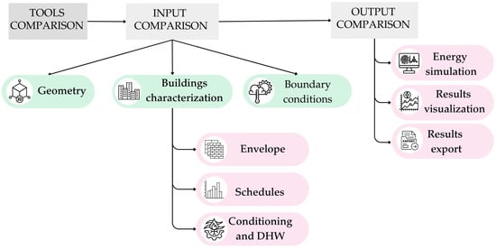
Figure 1.
Methodological workflow.
Geometry encompasses data related to buildings, such as footprints, heights, window-to-wall ratios (WWRs), and the number of storeys, and data related to the characteristics of the area, like the terrain altitude and green and blue infrastructure. The primary objective of collecting such data is to generate accurate urban 3D models for subsequent simulations [12]. These models can be developed using various data sources, including existing geospatial databases [13], Light Detection and Ranging (LiDAR) [14], and oblique photogrammetry [15,16,17], each offering different levels of accuracy and coverage.
Building characterisation involves the definition archetypes or prototype (standard fully characterised buildings models) [18,19,20], which encompass envelope properties; occupancy schedules; and heating, ventilation, air conditioning, and domestic hot water (DHW) systems and operating conditions. The acquisition of archetype-related data can be achieved through the use of statistical open-source datasets [13], such as cadastre data [21] and Energy Performance Certificates (EPCs) [22,23,24], which provide information on the building use category, floor area, year of construction or major renovation, heating system type, energy carrier, and standardised energy performance indicators (e.g., heating demand in kWh/m2 per year) [22,23,24]. Alternatively, data can be obtained through the use of measured data [19], leveraging statistical or machine learning techniques to enhance accuracy and reliability. A precise definition of these archetypes is crucial, as it directly influences the predictive accuracy of UBEM simulations.
Following the input definition, an output comparison is conducted to assess the impact of different input choices on the energy simulation results. The comparison is conducted using two distinct test cases—cases A and B—to examine how variations in the input selection and calculation methods of each tool influence simulation results. Case A investigates the impact of software constraints by using distinct datasets for schedules, internal loads, and DHW system efficiency, reflecting the intrinsic characteristics of each tool. This setup highlights how software limitations can shape user choices and affect outputs. Conversely, case B minimises user-induced discrepancies by ensuring that input parameters, such as envelope characterisation, schedules, and internal load, are as similar as possible across both tools. This approach isolates differences arising from the computational models themselves rather than from input variations. Ultimately, this dual-case methodology underscores the sensitivity of UBEM models to both tool-specific constraints and input parameter selection. Additionally, the output comparison examines result visualisation and data export options [25], evaluating how different tools represent and communicate simulation outcomes. Effective visualisation techniques and structured export formats are essential for facilitating result interpretation, enabling cross-tool validation, and supporting informed decision making in urban energy planning.
This structured methodology ensures a comprehensive evaluation of UBEM tools, enabling an objective comparison of their capabilities, performance, and applicability in UBEM.
3. Case Study
To evaluate the capabilities of the tool, the proposed methodological framework was employed in the analysis of a district located in the northeast of Milan, Italy, as presented in Figure 2. The case study was selected by AMAT, the Municipality-owned Agency for Mobility, Environment and Territory Agency, to asses which simulation tools could be used for studies of urban decarbonisation using a real case study.
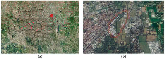
Figure 2.
Crescenzago district: (a) aerial view of Milan, Italy, with the district of interest highlighted; (b) a zoomed-in view of the highlighted district. The red line indicates the boundaries of the study area.
The case study includes 59 buildings, primarily consisting of residential and office structures constructed between 1946 and 2006. Figure 3 presents the distribution of building typologies and construction periods within the district, emphasizing the diversity of the building stock.
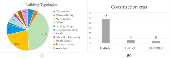
Figure 3.
Overview of Crescenzago district: (a) classification of building typologies; (b) construction periods.
The input data necessary to fully characterise the case study in both the selected UBEM tools were gathered from a range of open-source datasets that include the following:
- Geospatial data sourced from OpenStreetMap (OSM) [26], providing a foundational layer for the spatial configuration of the model and buildings footprints, as well as the urban layout;
- Building envelope characteristics obtained from Certifcazione ENergetica degli EDifci (CEER/CENED) [27], a regional collection of energy performance certificates (EPCs), offering detailed insights into the thermal properties of buildings within the study area;
- Heating and domestic hot water system data collected from CURIT [28], a database established by the Lombardy Region in 2008 to collect and manage information on heating and cooling generation systems in buildings;
- Climatic data in EPW format from Climate.oneBuilding [29]. The selected file corresponds to a Typical Meteorological Year (TMY) [30] for the Milan-Linate weather station (ITA_LM_Milano-Linate.AP.160800_TMYx), derived from historical hourly data. TMY files are downloaded by selecting the country and location of interest on the platform, which provides pre-processed, simulation-ready datasets based on verified meteorological sources. The EPW file includes key environmental variables such as the dry-bulb and dew-point temperature, relative humidity, atmospheric pressure, direct and diffuse solar radiation, global horizontal irradiance, wind speed and direction, cloud cover, precipitation, and snow cover. These variables enable hourly-resolution simulations of building energy performance under typical climatic conditions [31].
3.1. Tool Description
In recent years, several tools for energy modelling at the urban scale have been developed and continue to be developed [9].
Among the tools available for UBEM, two bottom-up, physics-based platforms are Integrated Computational Design (iCD) [32], which is currently the only commercially available UBEM tool, provided by the Integrated Environment Solutions (IES) company [33], and the Urban Modelling Interface (umi) [34], currently one of the most commonly used tools in the research field.
iCD is a 3D master planning modelling tool that is suitable for application in both new developments and retrofit initiatives, offering energy analysis outcomes through its Virtual Environment (VE) simulation engine [31]. The calculation methodologies of iCD are the same as for the operation of IES-VE [33] in the simplified Apache System version.
umi represents a multi-year effort by the MIT Sustainable Design Lab to develop an urban modelling design platform with abilities to evaluate operational building energy use, sustainable transportation choices, daylighting, and outdoor comfort at the neighbourhood and city levels [34]. The tool is an open-source design environment for Rhinoceros 3D (Rhino) [35], and it is frequently updated to maintain compatibility with the latest Rhino releases. It includes an Application Programming Interface (API) for researchers and consultants interested in adding additional performance modules and metrics. Focus users are urban planners, municipalities, utilities, sustainability consultants, and other urban stakeholders [36].
3.2. Input Description
3.2.1. Geometry
In UBEM, the definition of building geometry serves as a foundational input, significantly influencing both the accuracy and computational performance of simulations [37]. Unlike traditional Building Energy Modelling (BEM), which often relies on detailed and highly resolved geometries, UBEM adopts simplified representations to enable modelling at larger scales—such as neighbourhoods, districts, or entire cities—while maintaining computational feasibility [38].
Most UBEM tools rely on the processing of open-source datasets [13], particularly integrating Geographic Information System (GIS) format files such as CityGML [39], GeoJSON, and Shapefile [40], as well as OpenStreetMap (OSM) data [41]. GIS formats are particularly practical, since they are widely used and have been standardised by municipalities to store building information [6].
In iCD, 3D building geometries can be generated using the following methods:
- By importing models directly from OpenStreetMap (OSM);
- By importing GIS files in .shp or .geojson format;
- By manually constructing 3D elements using polygon-based tools within the interface.
In umi, direct integration with OSM is not available. However, GIS file integration is supported by the UBEM TOOLkit [42], which converts GIS files into the .uio format compatible with the umi platform. Additionally, umi allows for manual creation of 3D building geometry using polygonal modelling tools within the Rhinoceros environment.
3.2.2. Building Characterisation
To streamline data input in UBEM, buildings are typically grouped via representative “archetypes”, “prototypes”, or “reference buildings” [43]. These archetypes are classified based on key indicators such as building end use (e.g., residential, office, or retail), geometric typology, and construction period [44].
The assignment process differs between iCD and umi. In iCD, building information is imported via a csv file, and archetypes are assigned using the “Query Tool”, allowing for an automated classification process [45]. In contrast, umi requires a manual approach, where the user individually selects each building and assigns it to an archetype family from a predefined template library [46]. This library follows a sequential waterfall structure, where each section must be completed before proceeding to the next, ensuring a structured but time-intensive workflow.
Building Envelope characteristics
In iCD, envelope archetypes are uploaded as CSV files. Users can define average U values for each envelope component (e.g., walls, roofs, and windows) but cannot modify predefined stratigraphies or material layers. In umi, users can customise the full stratigraphy of opaque components, defining individual materials and their thicknesses. However, for glazing elements, umi only allows the specification of an overall U value for a window (without the distinction between the glass and the frame)
Schedules
iCD includes a selection of predefined occupancy schedules based on ASHRAE standards [47], assigned by building type. These schedules define daily and weekly patterns for heating, cooling, domestic hot water (DHW), and occupancy but do not account for annual or seasonal variability. umi offers user the possibility of creating, editing, and visualising occupancy schedules on daily, weekly, and annual bases. Users manually input values for each hour, allowing for detailed customisation over the full year. Both tools require users to define usage schedules and power density values for lighting and equipment. In umi, these schedules are fully customisable; in iCD, they are selected from predefined options.
Conditioning and DHW
Both tools use system efficiency values to calculate heating and cooling energy consumption. For DHW, umi requires the input of peak flow rates and supply temperatures, whereas iCD uses a system efficiency parameter. umi allows for detailed scheduling of system operations across the year; iCD limits users to predefined non-annual schedules.
In both platforms, energy carriers (e.g., electricity and gas) and technologies (e.g., heat pumps and boilers) can be defined but do not influence energy simulation results. These inputs serve only as post-simulation metrics, such as in emissions calculations.
3.2.3. Boundary Conditions
To represent prevailing climatic conditions, UBEM methods typically rely on a single, citywide annual weather dataset, most commonly in the form of a Typical Meteorological Year (TMY) [48]. These TMY files provide hourly environmental variables for a given location, including solar radiation, dry-bulb temperature, relative humidity, wind speed, and wind direction [49].
However, since TMY data are statistically derived rather than being based on actual weather records from a specific year, they cannot capture climate extremes or short-term variations that may occur at a given site [50]. To address this limitation, UBEM workflows can integrate alternative climatic datasets, such as historical weather data or future weather projections, to better reflect climate variability and long-term trends [12].
A key constraint of the analysed UBEM tools is their strict requirement for weather data to be formatted in EnergyPlus Weather (EPW) format [29], which may necessitate additional data processing when integrating non-standard climate datasets.
However, in this regard, the two tools do not differ significantly, as both allow for the integration of any type of climate file. The main distinction lies in umi’s Urban Weather Generator (UWG), which estimates the hourly urban canopy air temperature and humidity using weather data from a rural weather station [51].
Concerning the assessment of solar gains, umi estimates incident solar radiation using a simplified shoebox-based model, distributing gains across façades based on typical building characteristics. In contrast, iCD uses predefined assumptions in default workflows but can optionally integrate more detailed solar simulations through the Suncast and Solar Assessment modules. In this study, solar gains were modelled using the default settings of each tool.
Table 1 summarises the analysed input parameters.

Table 1.
Summary table of the input comparison.
4. Results and Discussion
This section delineates the differences and constraints emerging from the comparison of the two investigated tools. The performed analysis does not serve as a validation of the models per se, since it does not involve a comparison with measurement data, but aims to explore the unique settings and outcomes offered by the two UBEM tools. This distinction is particularly relevant at the urban scale, where different tools may yield similar temporally and spatially aggregated energy use estimates (e.g., yearly results at the city level) while relying on significantly different underlying modelling assumptions and calculation models. Furthermore, the choice of modelling approach can substantially influence the granularity and reliability of simulation outputs [19].
4.1. Tool Comparison
In this section, we compare the iCD and umi tools with respect to their energy calculation methodologies, focusing on how each handles thermal zoning, system assumptions, and simulation workflows at the urban scale. Although both tools are intended for district- and neighbourhood-level analyses, they rely on different modelling strategies and levels of abstraction. Notably, iCD leverages the IES-VE engine [52], while umi adopts a streamlined approach based on simplified representations.
In particular, the IES-VE engine, in the simplified Apache system calculation method, enables energy modelling of individual buildings, accounting for a range of influencing factors, such as thermal properties of the building envelope, occupancy patterns, HVAC system characteristics, and climate data. For assessment of heating and cooling energy demands, IES-VE employs a heat-balance approach that evaluates both sensible and latent heat flows entering and exiting each air mass and building surface within a defined thermal zone [35]. To reduce computational effort in the iCD workflow, each geometry is represented as a single thermal zone. The calculation of final energy consumption incorporates the efficiencies of the building’s energy systems, thereby accounting for generation and distribution losses to estimate actual energy use more accurately [35].
In contrast, umi is initially designed to operate at an urban scale and adopts a computationally efficient modelling approach suitable for district- and neighbourhood-level assessments. To this end, umi utilises a simplified method based on the “umi Shoeboxer” algorithm, which abstracts each building typology as a reduced representation comprising a limited number of thermal zones. Typically, this includes two zones: a perimeter zone, representing regularly conditioned spaces such as dwellings or offices, and a core zone, which captures unconditioned or intermittently conditioned spaces like stairwells, lift shafts, or service areas. This distinction assumes that the perimeter zone is the primary interface for solar gains and external heat exchange, while the core zone remains comparatively thermally stable due to its internal location.
Shoebox geometries are generated from a defined set of inputs, including the building footprint, number of storeys, floor-to-ceiling height, window-to-wall ratio, and basic envelope characteristics. Internal gains, occupancy profiles, and HVAC configurations are assigned based on standard templates aligned with building use types (e.g., residential or office) [53]. The information is subsequently exported to Input Data File format for energy simulation with EnergyPlus [54].
Both iCD and umi are UBEM tools designed to support district- and neighbourhood-scale energy assessments through archetype-based modelling. While the two platforms share a common conceptual foundation, they diverge significantly in how archetypes are implemented, how thermal zones are structured, and the level of user control provided in the modelling process.
From a theoretical standpoint, iCD enables a higher degree of consistency and repeatability across large datasets, making it suitable for policy-level simulations or district energy planning. However, its simplified zoning and rigid input structures may limit its applicability for in-depth analyses of complex buildings or retrofit scenarios. umi, on the other hand, provides a more flexible and modular environment but requires more manual input, which may slow down project development when hundreds or thousands of buildings are involved.
Table 2 summarises the general pros and cons of iCD and umi.
Table 2.
Pros and cons iCD and umi.
4.2. Input Comparison
4.2.1. Geometry
The two tools adopt different approaches for building geometry input, with implications for usability, scalability, and integration with existing datasets.
iCD offers a high degree of flexibility by supporting multiple methods of generating 3D building geometries. Users can import data directly from OpenStreetMap (OSM), work with standard GIS formats such as .shp and. geojson, or create geometries manually from polygons. This range of options allows iCD to integrate widely used urban data sources, particularly those managed by local authorities or planning departments. The ability to use OSM data without pre-processing is especially valuable, as it significantly reduces the time and technical expertise required to prepare spatial data. This makes iCD particularly advantageous for projects where data come from diverse or standardised municipal sources or where batch processing of large building stocks is essential.
In contrast, umi does not support direct integration with OSM. GIS data can only be imported after being converted into a .uio file format using the UBEM TOOLkit [42], which introduces an extra layer of complexity and may require additional technical steps. Although umi offers manual geometry creation within the Rhinoceros environment, which allows for fine-grained control of individual building forms, this method is less efficient when dealing with large datasets. The reliance on Rhino also limits the accessibility of the tool to users who are already proficient in that platform and who are working on smaller-scale or design-oriented studies where manual refinement is feasible.
While both platforms ultimately depend on GIS data as the primary input for geometry, their workflows differ in terms of native file compatibility, pre-processing requirements, and automation potential. From a practical standpoint, iCD is better suited to projects that prioritise speed, scalability, and integration with standard urban datasets, whereas umi is more appropriate for case studies that require detailed manual modelling or design flexibility at the individual building level.
Figure 4 shows the 3D models. The first one is in iCD, in which OSM is exploited for the creation of the geometry, and the second one is in umi, in which the UBEMToolkit is instead exploited.
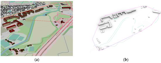
Figure 4.
Three-dimensional model of the case study in (a) the iCD environment and (b) the umi environment.
4.2.2. Building Characterisation
iCD streamlines the archetype assignment process through the use of CSV-based data importation and an integrated query tool, enabling automated classification of buildings. This approach facilitates batch processing, allowing multiple buildings to be assigned archetypes simultaneously based on user-defined queries. Moreover, the CSV format lends itself to integration with external tools—such as MATLAB [55], Python [56], or other data processing environments—supporting the pre-processing and generation of classification schemas prior to importation. This makes iCD particularly well-suited for projects involving extensive datasets or advanced scripting workflows, as it minimises manual intervention and enhances scalability.
In contrast, umi adopts a manual assignment workflow, requiring users to individually select each building and link it to an archetype from a predefined template library. This system is structured via a sequential waterfall interface, which enforces order and completeness but results in a more time-intensive and user-dependent process. While this method ensures a structured and comprehensive modelling approach, it is more time-consuming and heavily reliant on user input, potentially limiting efficiency when working with large or complex building stocks.
Building Envelope characteristics
For the assignment of envelope archetypes, iCD allows users to upload a csv file. However, it introduces limitations that may affect model accuracy: users cannot modify the predefined stratigraphies or create fully customised layer arrangements by adjusting material order. The only available option is to set a specific average thermal transmittance (U value) of the component (such as and external wall, window, or roof), without the ability to modify other parameters influencing the dynamic thermal behaviour of the envelope, such as thermal mass. Additionally, the predefined stratigraphies in iCD are tailored to a North American context, which may not align with the geographical conditions of other areas (such as the one analysed in this study).
These limitations have significant implications for model outputs. The inability to control the thermal capacity of the envelope affects the dynamic thermal performance of the building. Moreover, the lack of stratigraphy customisation prevents detailed material studies for retrofit scenarios and inhibits assessments of embodied carbon, which are critical for evaluating the sustainability of building envelope solutions [57].
Conversely, umi offers flexibility for the modelling of opaque envelope components, allowing users to define a fully customised stratigraphy, specifying individual material properties and thicknesses. However, it presents limitations in glazing modelling, as it only allows for the overall average thermal transmittance of the window to be set, without distinguishing between the glass and the frame, treating them as a single entity rather than separate elements. The limitations in glazing modelling may impact the accuracy of thermal performance predictions, which may result in an overestimation or underestimation of overall window performance, particularly in scenarios where the frame’s thermal characteristics significantly differ from those of the glazing. Consequently, this limitation could affect heating and cooling load estimations, as well as daylighting and solar gain analyses.
Schedules
Accurately modelling occupants’ behaviour (OB) is crucial for understanding and predicting a building’s energy performance [58]. Despite the uncertainty in building performance introduced by occupants, both presence and actions are usually modelled in very simplistic ways [59]. Common modelling approaches include the use of basic schedules; typical power densities; and, at most, simple rules about how occupants use equipment, lighting, and other energy systems of the building [60]. The OB capabilities of the two tools differ significantly in terms of customisation and visualisation. iCD offers a limited selection of predefined occupancy schedules, differentiated by per building end-use type, based on ASHRAE standards [47], without the possibility for user-defined modifications or graphical visualisation. The tool provides daily and weekly variations for heating, cooling, DHW, and occupancy schedules that can be associated with each archetype and an occupancy density parameter to estimate the actual number of occupants. However, it lacks annual variability, preventing adjustments that account for seasonal changes.
In contrast, umi offers a greater degree of flexibility, allowing users to create, modify, and visualise detailed daily, weekly, and yearly occupancy schedules. However, this high level of customisation can be time-consuming, as schedules must be manually inputted. Users are required to set a value for each hour and to create a fully diversified annual schedule, requiring them to define up to 365 different daily values, specifying a value for every hour interval.
In terms of lighting and equipment, both tools require use schedules (which can be fully personalised in umi) and a power density factor.
Conditioning and DHW
The two tools adopt a similar approach for heating and cooling systems: an efficiency value is assigned to the system to compute energy use based on energy needs. However, their methodologies for defining DHW consumption differ, since umi relies on the setting of the peak flow rate and the supply temperatures, while iCD requires the definition of system efficiency. The main difference between the two tools lies in the operating schedules of the conditioning systems. While umi allows users to define detailed daily, weekly, and annual schedules, iCD, in contrast, only offers a choice from a predefined list of schedules, which are not specified on an annual basis. This limitation prevents users from adhering to local standards and may lead to an overestimation of heating and cooling demands, as system operation is determined solely by the set-point temperature.
Both platforms allow users to specify energy carriers (e.g., natural gas, electricity) and technologies (e.g., boiler, heat pump). However, these inputs do not influence the actual energy simulation, which is solely based on the efficiency or coefficient of performance (COP) defined by the user. Neither tool establishes a direct link between the technology type and efficiency values, which may lead to inconsistencies in building templates if unrealistic combinations are assigned. The inclusion of energy carriers in iCD serves post-simulation analyses, such as CO2; emissions assessments, rather than influencing the core energy simulation process.
4.2.3. Boundary Conditions
Both iCD and umi require weather data to be formatted in the EnergyPlus Weather (EPW) format. While this ensures compatibility with energy simulation engines, it may necessitate data processing when using non-standard datasets.
Both tools are compatible with alternative climatic inputs, such as historical datasets or future climate projections, if they are converted into EPW format.
While both tools accept standard weather files, umi includes an additional feature: the Urban Weather Generator (UWG). This component estimates the urban canopy air temperature and humidity by adjusting rural weather station data, capturing the effects of the urban heat island phenomenon. Given that UBEM tools are explicitly designed to support urban-scale energy planning and policy development, the ability to represent localised climatic conditions is of critical importance. Conventional weather files often fail to capture intra-urban temperature variations, especially during periods of climatic extremes. As such, integrating UHI effects—through the use of tools like the UWG—enhances the relevance and applicability of simulation results for urban planners by providing more realistic estimations of cooling demand, thermal comfort, and peak loads in dense urban contexts.
By incorporating this urban microclimate layer, umi strengthens its utility as a decision-support tool for sustainable urban design, enabling more accurate assessments of climate resilience and adaptation strategies at the neighbourhood and city scales.
4.3. Output Comparison
4.3.1. Energy Simulations
This section examines the differences and constraints of the two investigated tools based on simulation results.
Simulations are conducted under two different scenarios:
- Case A: Distinct datasets are used for schedules, internal loads, and DHW system efficiency. This distinction is a result of the tools’ intrinsic characteristics; umi can adopt UNI 13790 standard [61] to align with the Italian case study, whereas because iCD does not allow for customisation, ASHRAE is employed [47]. This scenario is set up to investigate how software limitations can influence user choices and, therefore, simulation results.
- Case B: The input data for the two tools, including envelope characterisation, schedules, and internal loads, are chosen to be as similar as possible. This scenario aims to identify the source of discrepancies between the two tools—whether they result from differences in input data or variations in the computational models used, minimizing the effect of user choices.
This analysis is crucial for not only understanding how user choices impact the final outcomes but also for assessing the tools’ flexibility in incorporating case study-specific input.
Figure 5 and Table 3 report the annual energy use of the district case study for various end uses (DHW, heating, equipment, and lighting) for both tools and both cases. Cooling energy use was not analysed in this study because data on cooling systems were not available and is, therefore, not included.
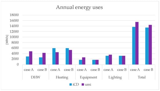
Figure 5.
Annual energy use for case A and case B.
Table 3.
Annual and total variation [%] * between case A and case B.
The total annual energy use was obtained as the sum of all the above-mentioned contributions, since the two simulation tools provide this value as Energy Use Intensity (EUI), although contributions from different energy carriers should not technically be summed.
It is evident that when comparing the two software tools solely in terms of total annual energy use of the district (i.e., the sum of all the various end-use contributions), differences are limited: 13% for case A and 7% for case B. However, when examining the individual energy use contributions, differences between the two software outputs rise to 66% for DHW in both cases A and B and 51% for heating in case A. This highlights how impactful discrepancies in the input data and calculation methods can be.
To gain deeper insights, additional analyses were conducted by examining monthly energy use outputs, providing a more detailed comparison of the tools’ performance at a finer temporal resolution.
Figure 6 offers a comparative analysis of DHW energy usage, illustrating significant differences in simulation outcomes:
- The discrepancy observed between cases A and B arises primarily due to umi’s ability to specify a peak flow rate. This feature cannot be added in iCD.
- The variation in iCD output between case A and case B can be attributed to differences in DHW efficiency. In case B, an ideal boiler (i.e., efficiency equal to 1) was simulated, mirroring the model used in umi, in contrast to the standard boiler efficiency (i.e., 0.85) applied in case A. This discrepancy arises because, in umi, the system’s efficiency can be altered solely by adjusting the supply water temperature, making it challenging to replicate the same efficiency utilised in iCD. Consequently, an ideal boiler was employed for simulation purposes.
- The consistent variability between the two software models throughout the year can be explained by the fact that DHW production is tied to the occupancy schedule, which remains static across months in iCD due to the inability to set a yearly schedule. For simplicity, this fixed schedule was also applied to umi simulations in both cases A and B.
- The difference in umi output between case A and case B is linked to the adoption of different occupancy schedules. Case A adheres to ISO 18523 [32], whereas case B follows the ASHRAE standards. These different schedules were adopted because iCD utilises predefined schedules based on building typology, which are not adjustable. The primary distinctions between ISO 18523 and ASHRAE standards in the context of occupancy schedules lie in their approach to temporal granularity and operational assumptions. ISO 18523 offers detailed daily schedules with hourly values, allowing for variations between weekdays and weekends, as well as seasonal changes. This level of detail enables a more precise representation of occupancy patterns. In contrast, ASHRAE standards provide more generalised schedules that may not explicitly account for daily or seasonal fluctuations, leading to a more uniform representation of occupancy over time [62]. As a result, when fixed annual schedules are applied—as in umi case A—DHW monthly energy needs tend to scale proportionally with the number of days in each month.

Figure 6.
DHW monthly energy use comparison.
Figure 7 shows the results in terms of heating energy use. The following notable distinctions can be highlighted:
- The discrepancy between cases A and B in both tools from April to October is due to umi’s ability to incorporate a yearly schedule, which enables it to adhere to local regulations that require heating to be turned off from 15 April to 15 October. In contrast, iCD operates based on set point temperatures and does not allow for such seasonal adjustment. Additionally, while attempting to harmonise inputs across both models, umi’s limitation in modelling windows—specifically, the exclusion of frames—significantly impacts the results. Moreover, even though external wall and roof stratigraphies were adjusted to match the U value, iCD compensates for discrepancies between the inputted U value and the actual performance of the chosen stratigraphy by adding insulation layers, resulting in a different dynamic behaviour of the envelope. For these simulations, the efficiency of the heating system was set to 0.85 in both tools.
- The variation in iCD output between cases A and B is minimal, since no changes were made in terms of schedule, efficiency, stratigraphy, or internal loads.
- The difference in heating energy use between umi cases can be traced to the use of different occupancy schedules and internal load values. Case A conforms to the ISO 18523 standard [32], whereas case B is based on ASHRAE standards. This is contrasted with iCD’s approach, which uses fixed schedules and internal loads determined by the building typology and does not allow for modification.

Figure 7.
Monthly heating energy use comparison.
Figure 8 and Figure 9 show comparisons in terms of equipment and lighting energy use and highlight the following observations:
- Case B scenarios exhibit identical values, as anticipated, due to the uniformity of inputs regarding schedule and equipment load for each building. Conversely, case A in umi shows divergent results due to modifications of the schedule and load following the ISO 18523 standards [63].

Figure 8.
Monthly equipment energy use comparison.

Figure 9.
Monthly lighting energy use comparison.
This illustrates the critical issue of how different tools, when applied to the same scenario with the same available data, can produce inconsistent results. These discrepancies are primarily due to variations in the models’ data assignment processes. Notably, the DHW and equipment energy use results show the greatest divergence and are, thus, the most misleading.
4.3.2. Results Visualisation
iCD and umi represent two different approaches to results visualisation, each offering functionalities for assessing energy performance. iCD provides an extensive set of tools designed for scenario analysis, comparative assessments, and high-resolution visualisation of urban energy data. Its automated reporting system delivers comprehensive energy breakdowns, while its interoperability with other tools of the IES suite, such as the iScan tool [64], allows for detailed building-level performance evaluation. A key aspect of iCD’s analytical capabilities is its scenario generation tool, which establishes a structured approach to modelling alternative urban energy conditions, enhancing the comparison of multiple simulation scenarios. Visualisation in iCD further strengthens its analytical depth by enabling the overlay of attribute data onto three-dimensional urban models. This approach supports object-level filtering, customisable data overlays, temporal trend analysis and the application of dynamic colour schemes to highlight variations in energy demand and urban morphology. Reporting functionalities in iCD are equally comprehensive, covering site-level characteristics, energy consumption metrics, water use distribution, urban planning data, photovoltaic integration, and time-series energy trends.
Conversely, umi offers an approach that integrates energy performance assessment directly within the design workflow, allowing users to visualise and interpret results within the modelling environment. Its visualisation capabilities include three-dimensional representations of urban energy dynamics and detailed performance indicators such as energy use intensity and daylight availability.
4.3.3. Exportation of the Results
In iCD, the csv export process includes several configurable options that enable users to tailor the output to specific analytical requirements. Key parameters such as the object identifier column and property units are preselected by default to ensure consistency and ease of interpretation. However, additional options can be adjusted to enhance data structuring and usability. Users can export feature types separately, include sub-level properties such as storey- or floorplate-specific data, incorporate uniform resource identifiers (URIs) for property names to maintain data traceability, and include latitude and longitude coordinates for spatial analysis. Other functionalities allow for the retention of empty columns to preserve dataset completeness or the aggregation of results to provide summarised performance metrics. In iCD, energy performance results are typically expressed in kWh/m2 per year.
Similarly, umi offers csv export functionalities that enable seamless data extraction for external evaluation. Through an interface, users can select specific energy performance metrics for export. The results exported from umi are presented in kWh or normalised in kWh/m2. Additionally, both iCD and umi allow for the export of detailed data related to various aspects of building performance, including system energy consumption (e.g., heating, cooling, and lighting) and thermal comfort analysis.
5. Conclusions
This study has presented a comparative analysis of two urban building energy modelling (UBEM) tools, iCD and umi, focusing on their modelling assumptions, input handling, and output behaviours. The motivation behind this research stems from the need to understand how different tools, although designed for similar purposes, can yield significantly divergent results when applied to the same case study.
A key methodological contribution is the development of a replicable framework for UBEM tool comparison that is applicable beyond the tools tested here. Applying this framework to iCD and umi revealed critical differences, particularly in how domestic hot water systems, envelope definitions, and internal load schedules are handled. These variations notably affect modelling outcomes, especially at higher temporal resolutions.
The findings highlight the following several limitations:
- umi’s DHW system efficiency, which can only be adjusted by modifying the supply water temperature, presenting challenges in defining the system’s overall efficiency.
- umi’s limited ability to define frame stratigraphy in window modelling affects the accuracy of simulation results.
- iCD automatically corrects discrepancies between inputted U values and actual stratigraphic performance by adding insulation layers, resulting in different dynamic behaviour of the building envelope.
- iCD adopts an inflexible approach to schedules and internal loads, which are pre-determined by the building typology, in stark contrast to umi’s incorporation of personalised yearly schedules.
These differences underscore the importance of tool-specific awareness when conducting UBEM studies.
Looking ahead, several areas require further research. Firstly, while this study offers useful insights, the simulations were not validated against empirical data. Future work should aim to compare simulation outcomes with real-world measurements, thereby enhancing the reliability of findings and identifying where and why discrepancies occur. However, this effort is currently hampered by the limited availability of high-quality energy use data at the urban scale, often due to privacy concerns and a lack of digitalisation in the built environment.
Another important direction involves testing how UBEM tools perform under future climate conditions and in conjunction with evolving energy production technologies. As cities aim for long-term sustainability, accurate modelling of energy supply and demand under changing environmental scenarios will become increasingly critical.
The scalability of UBEM tools also deserves closer scrutiny. The current case study was limited in scope, and future investigations should examine how these platforms perform when applied to larger urban areas with diverse building typologies. Such studies would offer valuable insights into the adaptability and computational robustness of UBEM tools in more complex settings.
Additionally, both iCD and umi could benefit from greater interoperability and enhanced data integration features. For example, direct importation of envelope characteristics from external databases—such as the URBEM library [65]—would improve consistency and streamline workflows. The ability to incorporate occupant behaviour (OB) schedules more seamlessly, ideally through the use of built-in stochastic generators, would further increase the realism and efficiency of energy simulations.
Ultimately, the development of a standardised approach for both input data and model calculations remains a transversal goal. Such standardisation would minimise discrepancies caused by differing modelling assumptions and improve the reliability of UBEM tools, contributing to a more data-driven and evidence-based approach to urban energy planning.
Author Contributions
Conceptualization, C.N., R.C., A.B., M.F. and F.C.; Methodology, C.N., R.C., A.B., M.F. and F.C.; Software, C.N. and R.C.; Formal analysis, C.N., R.C. and A.B.; Writing—original draft, C.N. and A.B.; Writing—review & editing, C.N., A.B., M.F., X.S. and F.C.; Supervision, F.C.; Project administration, F.C.; Funding acquisition, F.C. All authors have read and agreed to the published version of the manuscript.
Funding
This study was developed partially within the framework of the URBEM project (PRIN, code: 2020ZWKXKE), which received funding from the Italian Ministry of University and Research (MUR), and partially under the National Recovery and Resilience Plan (NRRP), Mission 4 Component 2 Investment 1.3—Call for tender No. 1561 of 11.10.2022 of Ministero dell’Università e della Ricerca (MUR); funded by the European Union–NextGenerationEU. Award Number: Project code PE0000021, Concession Decree No. 1561 of 11.10.2022 adopted by Ministero dell’Università e della Ricerca (MUR), CUPC93C22005230007, according to attachment E of Decree No. 1561/2022, Project title “Network 4 Energy Sustainable Transition—NEST”.
Data Availability Statement
The original contributions presented in the study are included in the article, further inquiries can be directed to the corresponding author.
Acknowledgments
The authors thank AMAT s.r.l., especially Eng. Marta Papetti, who was the main contact, for supporting the research by providing data to develop the case study.
Conflicts of Interest
The authors declare no conflicts of interest.
References
- Suppa, A.R.; Ballarini, I. Supporting climate-neutral cities with urban energy modeling: A review of building retrofit scenarios, focused on decision-making, energy and environmental performance, and cost. Sustain. Cities Soc. 2023, 98, 104832. [Google Scholar] [CrossRef]
- Allegrini, J.; Orehounig, K.; Mavromatidis, G.; Ruesch, F.; Dorer, V.; Evins, R. A review of modelling approaches and tools for the simulation of district-scale energy systems. Renew. Sustain. Energy Rev. 2015, 52, 1391–1404. [Google Scholar] [CrossRef]
- Fathi, S.; Srinivasan, R.; Fenner, A.; Fathi, S. Machine learning applications in urban building energy performance forecasting: A systematic review. Renew. Sustain. Energy Rev. 2020, 133, 110287. [Google Scholar] [CrossRef]
- Tatti, A.; Ferroni, S.; Ferrando, M.; Motta, M.; Causone, F. The Emerging Trends of Renewable Energy Communities’ Development in Italy. Sustainability 2023, 15, 6792. [Google Scholar] [CrossRef]
- Hong, T.; Chen, Y.; Luo, X.; Luo, N.; Lee, S.H. Ten questions on urban building energy modeling. Build. Environ. 2020, 168, 106508. [Google Scholar] [CrossRef]
- Ferrando, M.; Causone, F.; Hong, T.; Chen, Y. Urban building energy modeling (UBEM) tools: A state-of-the-art review of bottom-up physics-based approaches. Sustain. Cities Soc. 2020, 62, 102408. [Google Scholar] [CrossRef]
- Shen, P.; Wang, H. Archetype building energy modeling approaches and applications: A review. Renew. Sustain. Energy Rev. 2024, 199, 114478. [Google Scholar] [CrossRef]
- Buckley, N.; Mills, G.; Reinhart, C.; Berzolla, Z.M. Using urban building energy modelling (UBEM) to support the new European Union’s Green Deal: Case study of Dublin Ireland. Energy Build. 2021, 247, 111115. [Google Scholar] [CrossRef]
- Ferrando, M.; Causone, F. An overview of urban building energy modelling (UBEM) tools. In Proceedings of the Building Simulation Conference Proceedings, Rome, Italy, 2–4 September 2019; pp. 3452–3459. Available online: https://www.scopus.com/inward/record.uri?eid=2-s2.0-85107046249&partnerID=40&md5=53bb2234237411520daca9b9410591cf (accessed on 2 April 2025).
- Causone, F.; Scoccia, R.; Pelle, M.; Colombo, P.; Motta, M.; Ferroni, S. Neighborhood Energy Modeling and Monitoring: A Case Study. Energies 2021, 14, 3716. [Google Scholar] [CrossRef]
- Crawley, D.B.; Hand, J.W.; Kummert, M.; Griffith, B.T. Contrasting the capabilities of building energy performance simulation programs. Build. Environ. 2008, 43, 661–673. [Google Scholar] [CrossRef]
- Wang, C.; Ferrando, M.; Causone, F.; Jin, X.; Zhou, X.; Shi, X. Data acquisition for urban building energy modeling: A review. Build. Environ. 2022, 217, 109056. [Google Scholar] [CrossRef]
- Deng, Z.; Chen, X.; Yang, J.; Chen, Y. Development of urban building energy models in Hong Kong based on open-source datasets. In Proceedings of the Building Simulation 2023: 18th Conference of IBPSA, Shanghai, China, 4–6 September 2023. [Google Scholar] [CrossRef]
- Bahu, J.-M.; Koch, A.; Kremers, E.; Murshed, S.M. Towards a 3D Spatial Urban Energy Modelling Approach. Int. J. 3-D Inf. Model. 2014, 3, 33–41. [Google Scholar] [CrossRef][Green Version]
- Wu, B.; Xie, L.; Hu, H.; Zhu, Q.; Yau, E. Integration of aerial oblique imagery and terrestrial imagery for optimized 3D modeling in urban areas. ISPRS J. Photogramm. Remote Sens. 2018, 139, 119–132. [Google Scholar] [CrossRef]
- Yalcin, G.; Selcuk, O. 3D City Modelling with Oblique Photogrammetry Method. Procedia Technol. 2015, 19, 424–431. [Google Scholar] [CrossRef]
- Sun, X.; Shen, S.; Hu, Z. Automatic building extraction from oblique aerial images. In Proceedings of the 2016 23rd International Conference on Pattern Recognition (ICPR), Cancun, Mexico, 4–8 December 2016; pp. 663–668. [Google Scholar] [CrossRef]
- Ballarini, I.; Corgnati, S.P.; Corrado, V. Use of reference buildings to assess the energy saving potentials of the residential building stock: The experience of TABULA project. Energy Policy 2014, 68, 273–284. [Google Scholar] [CrossRef]
- Ferrando, M.; Ferroni, S.; Pelle, M.; Tatti, A.; Erba, S.; Shi, X.; Causone, F. UBEM’s archetypes improvement via data-driven occupant-related schedules randomly distributed and their impact assessment. Sustain. Cities Soc. 2022, 87, 104164. [Google Scholar] [CrossRef]
- Carnieletto, L.; Ferrando, M.; Teso, L.; Sun, K.; Zhang, W.; Causone, F.; Romagnoni, P.; Zarrella, A.; Hong, T. Italian prototype building models for urban scale building performance simulation. Build. Environ. 2021, 192, 107590. [Google Scholar] [CrossRef]
- Borges, P.; Travesset-Baro, O.; Pages-Ramon, A. Hybrid approach to representative building archetypes development for urban models—A case study in Andorra. Build. Environ. 2022, 215, 108958. [Google Scholar] [CrossRef]
- Dall’O’, G.; Sarto, L.; Sanna, N.; Tonetti, V.; Ventura, M. On the use of an energy certification database to create indicators for energy planning purposes: Application in northern Italy. Energy Policy 2015, 85, 207–217. [Google Scholar] [CrossRef]
- Österbring, M.; Mata, É.; Thuvander, L.; Mangold, M.; Johnsson, F.; Wallbaum, H. A differentiated description of building-stocks for a georeferenced urban bottom-up building-stock model. Energy Build. 2016, 120, 78–84. [Google Scholar] [CrossRef]
- Johari, F.; Shadram, F.; Widén, J. Urban building energy modeling from geo-referenced energy performance certificate data: Development, calibration, and validation. Sustain. Cities Soc. 2023, 96, 104664. [Google Scholar] [CrossRef]
- Malhotra, A.; Bischof, J.; Nichersu, A.; Häfele, K.-H.; Exenberger, J.; Sood, D.; Allan, J.; Frisch, J.; van Treeck, C.; O’Donnell, J.; et al. Information modelling for urban building energy simulation—A taxonomic review. Build. Environ. 2022, 208, 108552. [Google Scholar] [CrossRef]
- Open Street Maps. Available online: https://www.openstreetmap.org/about (accessed on 2 April 2025).
- Azienda Regionale per l’Innovazione e gli Acquisti S.p.A.-Lombardy Region, Certificazione ENergetica Degli Edifici. Available online: https://www.cened.it/home/ (accessed on 2 April 2025).
- Azienda Regionale per l’Innovazione e gli Acquisti S.p.A.-Lombardy Region, Catasto Impianti Termici Lombardia. Available online: https://www.curit.it/il-curit (accessed on 2 April 2025).
- Climate.OneBuilding, Energy Plus Weather File. Available online: https://climate.onebuilding.org/ (accessed on 2 April 2025).
- Evola, G.; Costanzo, V.; Infantone, M.; Marletta, L. Typical-year and multi-year building energy simulation approaches: A critical comparison. Energy 2021, 219, 119591. [Google Scholar] [CrossRef]
- Crawley, D.B.; Lawrie, L.K.; Winkelmann, F.C.; Buhl, W.F.; Huang, Y.J.; Pedersen, C.O.; Strand, R.K.; Liesen, R.J.; Fisher, D.E.; Witte, M.J.; et al. EnergyPlus: Creating a new-generation building energy simulation program. Energy Build. 2001, 33, 319–331. [Google Scholar] [CrossRef]
- Integrated Environmental Solutions, iCD Intelligent Community Design. Available online: https://www.iesve.com/products/icd (accessed on 2 April 2025).
- Integrated Environmental Solutions, About IES. Available online: https://www.iesve.com/about (accessed on 2 April 2025).
- Reinhart, C.; Dogan, T.; Jakubiec, A.; Rakha, T.; Sang, A. Umi—An Urban Simulation Environment for Building Energy Use, Daylighting and Walkability. In Proceedings of the Building Simulation 2013: 13th Conference of IBPSA, Chambery, France, 25–28 August 2013. [Google Scholar] [CrossRef]
- Robert McNeel & Associates. Rhino 8. Available online: https://www.rhino3d.com (accessed on 2 April 2025).
- MIT. Urban Modelling Interface. Available online: https://web.mit.edu/sustainabledesignlab/ (accessed on 2 April 2025).
- Xi, H.; Zhang, Q.; Ren, Z.; Li, G.; Chen, Y. Urban Building Energy Modeling with Parameterized Geometry and Detailed Thermal Zones for Complex Building Types. Buildings 2023, 13, 2675. [Google Scholar] [CrossRef]
- Salvalai, G.; Zhu, Y.; Sesana, M.M. From building energy modeling to urban building energy modeling: A review of recent research trend and simulation tools. Energy Build. 2024, 319, 114500. [Google Scholar] [CrossRef]
- Malhotra, A.; Raming, S.; Schildt, M.; Frisch, J.; van Treeck, C. CityGML model generation using parametric interpolations. Proc. Inst. Civ. Eng.-Smart Infrastruct. Constr. 2022, 174, 102–120. [Google Scholar] [CrossRef]
- Ang, Y.Q.; Berzolla, Z.M.; Reinhart, C.F. From concept to application: A review of use cases in urban building energy modeling. Appl. Energy 2020, 279, 115738. [Google Scholar] [CrossRef]
- OpenStreetMap. Available online: https://www.openstreetmap.org/#map=15/45.5034/9.2481 (accessed on 2 April 2025).
- Sustainable Design Lab. The UBEM Toolkit Provides a Myriad of Tools for Different Stakeholders. Available online: https://www.ubem.io/ubem-toolkit (accessed on 2 April 2025).
- Cerezo, C.; Sokol, J.; AlKhaled, S.; Reinhart, C.; Al-Mumin, A.; Hajiah, A. Comparison of four building archetype characterization methods in urban building energy modeling (UBEM): A residential case study in Kuwait City. Energy Build. 2017, 154, 321–334. [Google Scholar] [CrossRef]
- Dall’O’, G.; Galante, A.; Torri, M. A methodology for the energy performance classification of residential building stock on an urban scale. Energy Build. 2012, 48, 211–219. [Google Scholar] [CrossRef]
- 2011–2023 Integrated Environmental Solutions, Query Tool. Available online: https://help.iesve.com/icd2024/ (accessed on 2 April 2025).
- MIT Sustainable Design Lab. Template Library. Available online: https://umidocs.readthedocs.io/en/latest/docs/model-setup-template.html (accessed on 2 April 2025).
- ASHRAE. ASHRAE Standards and Guidelines. Available online: https://www.ashrae.org/technical-resources/standards-and-guidelines (accessed on 2 April 2025).
- Climate.onebuilding, TRY-Italia. Available online: https://climate.onebuilding.org/WMO_Region_6_Europe/ITA_Italy/index.html (accessed on 2 April 2025).
- Davila, C.C.; Reinhart, C.F.; Bemis, J.L. Modeling Boston: A workflow for the efficient generation and maintenance of urban building energy models from existing geospatial datasets. Energy 2016, 117, 237–250. [Google Scholar] [CrossRef]
- Li, W.; Zhou, Y.; Cetin, K.S.; Yu, S.; Wang, Y.; Liang, B. Developing a landscape of urban building energy use with improved spatiotemporal representations in a cool-humid climate. Build. Environ. 2018, 136, 107–117. [Google Scholar] [CrossRef]
- Urban Microclimate. Urban Weather Generator 4.1 Urban Heat Island Effect Modeling Software. Available online: https://urbanmicroclimate.scripts.mit.edu/uwg.php (accessed on 2 April 2025).
- IES-VE Calculation Methods. Available online: https://help.iesve.com/ve2021/ (accessed on 2 April 2025).
- Dogan, T.; Reinhart, C. Shoeboxer: An algorithm for abstracted rapid multi-zone urban building energy model generation and simulation. Energy Build. 2017, 140, 140–153. [Google Scholar] [CrossRef]
- U.S. Department of Energy. EnergyPlusTM Version 24.1.0 Documentation-Engineering Reference. Available online: https://energyplus.net/assets/nrel_custom/pdfs/pdfs_v24.1.0/EngineeringReference.pdf (accessed on 2 April 2025).
- MATLAB, version R2023a; The MathWorks Inc.: Natick, MA, USA, 2023.
- Python Language Reference, version 3.10; Python Software Foundation: Wilmington, DE, USA, 2023. Available online: https://www.python.org (accessed on 2 April 2025).
- Li, Y.; Feng, H. Integrating urban building energy modeling (UBEM) and urban-building environmental impact assessment (UB-EIA) for sustainable urban development: A comprehensive review. Renew. Sustain. Energy Rev. 2025, 213, 115471. [Google Scholar] [CrossRef]
- Carlucci, S.; De Simone, M.; Firth, S.K.; Kjærgaard, M.B.; Markovic, R.; Rahaman, M.S.; Annaqeeb, M.K.; Biandrate, S.; Das, A.; Dziedzic, J.W.; et al. Modeling occupant behavior in buildings. Build. Environ. 2020, 174, 106768. [Google Scholar] [CrossRef]
- Gunay, B. Mitigating office performance uncertainty of occupant use of window blinds and lighting using robust design. Build. Simul. 2015, 8, 621–636. [Google Scholar] [CrossRef]
- O’Brien, W.; Gaetani, I.; Gilani, S.; Carlucci, S.; Hoes, P.-J.; Hensen, J. International survey on current occupant modelling approaches in building performance simulation. J. Build. Perform. Simul. 2017, 10, 653–671. [Google Scholar] [CrossRef]
- UNI 13790; Prestazione Energetica Degli Edifici—Calcolo del Fabbisogno di Energia per il Riscaldamento e il Raffrescamento. Ente Italiano di Normazione: Milano, Italy, 2015.
- Ferrari, S.; Zagarella, F.; Caputo, P.; Bonomolo, M. Internal heat loads profiles for buildings’ energy modelling: Comparison of different standards. Sustain. Cities Soc. 2023, 89, 104306. [Google Scholar] [CrossRef]
- ISO 18523; Energy Performance of Buildings Schedule and Condition of Building, Zone and Space Usage for Energy Calculation. ISO: Geneve, Switzerland, 2018.
- IES—Integrated Environmental Solutions, iSCAN Building Data Analysis Make Sense of Operational Data to Improve In-Use Energy & Carbon Performance. Available online: https://www.iesve.com/products/iscan (accessed on 2 April 2025).
- URBEM—Urban Reference Buildings for Energy Modelling. Available online: https://www.urbem.polimi.it/databasedifici/ (accessed on 2 April 2025).
Disclaimer/Publisher’s Note: The statements, opinions and data contained in all publications are solely those of the individual author(s) and contributor(s) and not of MDPI and/or the editor(s). MDPI and/or the editor(s) disclaim responsibility for any injury to people or property resulting from any ideas, methods, instructions or products referred to in the content. |
© 2025 by the authors. Licensee MDPI, Basel, Switzerland. This article is an open access article distributed under the terms and conditions of the Creative Commons Attribution (CC BY) license (https://creativecommons.org/licenses/by/4.0/).