Fast and Interpretable Probabilistic Solar Power Forecasting via a Multi-Observation Non-Homogeneous Hidden Markov Model

Abstract

The increasing complexity and uncertainty associated with high renewable energy penetration require forecasting methods that provide more comprehensive information for risk analysis and energy management. This paper proposes a novel probabilistic forecasting model for solar power generation based on a non-homogeneous multi-observation Hidden Markov Model (HMM). The model is purely data-driven, free from restrictive assumptions, and features a lightweight structure that enables fast updates and transparent reasoning—offering a practical alternative to computationally intensive neural network approaches. The proposed framework is first formalized through an extension of the classical HMM and the derivation of its core inference procedures. A method for estimating the probability density distribution of solar power output is introduced, from which point forecasts are extracted. Thirteen model variants with different observation-dependency structures are constructed and evaluated using real PV operational data. Experimental results validate the model’s effectiveness in generating both prediction intervals and point forecasts, while also highlighting the influence of observation correlation on forecasting performance. The proposed approach demonstrates strong potential for real-time solar power forecasting in modern power systems, particularly where speed, adaptability, and interpretability are critical.

1. Introduction

The remarkable advantages of photovoltaic (PV) systems—such as flexible deployment, renewability, high reliability, and ongoing cost reductions—have rendered them increasingly competitive compared to other power generation methods. This trend has led to explosive growth in global PV installed capacity, underscoring the critical role of solar PV in transforming the worldwide energy sector. In 2024, global photovoltaic (PV) power generation surpassed 2000 TWh, marking a 30% increase compared to the previous year and accounting for approximately 7% of the world’s total electricity production. China played a pivotal role in this growth, contributing 41% of the global solar electricity output and achieving a 44% year-over-year increase in its solar generation [1,2]. Despite this rapid expansion, however, the security of the electricity supply and power dispatch face escalating challenges under high PV penetration scenarios.

Effective integration of photovoltaic (PV) generation into the power grid requires advanced scheduling and control strategies to ensure the safety, stability, and reliability of grid operations. In theory, the solar irradiance at any given location and time can be precisely determined based on astronomical models that account for the Earth’s position relative to the Sun. Using established physical and empirical conversion formulas, the corresponding PV power output can then be calculated. However, in real-world applications, the prediction of solar irradiance is subject to significant uncertainty due to the inherently chaotic and non-deterministic behavior of atmospheric conditions. Transient weather phenomena—such as cloud movement, aerosol concentration, and humidity variations—introduce rapid fluctuations that are difficult to capture accurately with deterministic models. Moreover, key meteorological factors such as ambient temperature, wind speed, and humidity also exert considerable influence on PV conversion efficiency and overall system performance [3,4,5]. These uncertainties, coupled with the intrinsic intermittency and variability of solar energy, pose substantial challenges to grid stability and hinder the seamless integration of high-penetration PV systems. To address these issues, the development of reliable and accurate PV forecasting techniques has become a focal point of research. An increasing number of studies by researchers, grid operators, and electricity market participants have sought to improve prediction accuracy across various time horizons, recognizing that precise forecasting is essential for real-time dispatch, reserve allocation, and market bidding strategies [6,7,8].

Depending on the specific requirements of end-users, photovoltaic (PV) power forecasting is typically categorized based on the forecasting time horizon. The most common classifications include day-ahead forecasting (short-term), intra-day forecasting (ultra-short-term), and medium- to long-term forecasting, each serving distinct operational and planning purposes within the power system [9]. For instance, day-ahead forecasts are essential for unit commitment and market bidding, while intra-day forecasts support real-time dispatch and reserve adjustments. Medium- and long-term forecasts are often used for capacity planning and investment decision-making. In response to these diverse needs, the past decade has witnessed a surge in research efforts aimed at developing advanced forecasting techniques tailored for PV systems [10,11]. These methods span a wide spectrum—from physical models based on solar geometry and numerical weather prediction (NWP) data, to statistical and machine learning approaches that exploit historical trends and real-time measurements. Despite this progress, the majority of existing studies have centered on generating deterministic, or point, forecasts that yield a single-valued estimate of future PV output. These point forecasts are typically optimized to minimize the error between predicted and observed values, and are widely used due to their simplicity and ease of interpretation. However, due to the inherent variability and uncertainty of solar resources, point forecasts are inevitably subject to deviations from actual observations. As a result, they provide limited insight into the range and likelihood of possible outcomes. For grid operators, energy traders, and other stakeholders operating in uncertainty-sensitive environments, such limited information is often insufficient for robust decision-making. This shortfall has motivated a growing interest in probabilistic forecasting methods, which offer richer information content by quantifying the uncertainty associated with future PV generation [12].

Probabilistic forecasting is a theoretical method that can quantify uncertainty in a stochastic process, which results can be issued in form of probability distributions, quantiles, or intervals, giving comprehensive information about the object [13,14,15]. In recent years, probabilistic forecasting methods have played an increasingly important role in the optimal design and scheduling of integrated energy systems, where decisions must be made under uncertainty arising from renewable power generation, load fluctuations, and market dynamics [16,17,18,19]. Additionally, it can also be summarized into point forecasts by the expectations, mode, or other analytical methods mentioned in related literature [20,21,22,23]. Some scholars obtain the probabilistic forecasting results by fitting the probability density distribution of forecast errors based on the historical data, while others directly obtain the distribution through statistical analysis methods such as bootstrapping. Although these proposed models proved effective, there are still some limitations. They are either too complex to apply in practice or based on assumptions that are difficult to verify in the application.

This paper proposes a novel probabilistic forecasting model (PFM) for solar power generation, built upon the Hidden Markov Model (HMM) framework, which falls under the category of purely statistical methods. Traditional HMMs rely on a small set of non-restrictive assumptions to describe the transformation relationships between latent states and observations, requiring only historical operational data of the target system. In the construction of the proposed PFM, solar power outputs and their associated meteorological variables are discretized into multiple intensity levels, which are mapped to the state and observation spaces of the HMM. To better capture real-world complexities, including system nonstationary and observation dependencies, the classical HMM is further extended into a family of non-homogeneous, multi-observation models with varying degrees of temporal and observational correlation. The proposed method offers a lightweight, computationally efficient, and easily interpretable framework that enables rapid updates and transparent probabilistic reasoning—making it particularly suitable for real-time applications and deployment in practical energy systems.

The paper is further organized as follows. In the next section, the basic concepts of HMM, derivation of extended HMMs, adopted methodology, and some practical result evaluation criteria are introduced. Section 3 describes the probability estimation procedure. Then, the comparative analysis of proposed extended HMMs is given in Section 4. Finally, the conclusions are presented in Section 5.

2. Theoretical Framework

In this section, the modeling process of the proposed method is introduced. In light of being a relatively new application in the field of solar power forecasting, some basic theories about the hidden Markov process will be described.

2.1. Hidden Markov Model

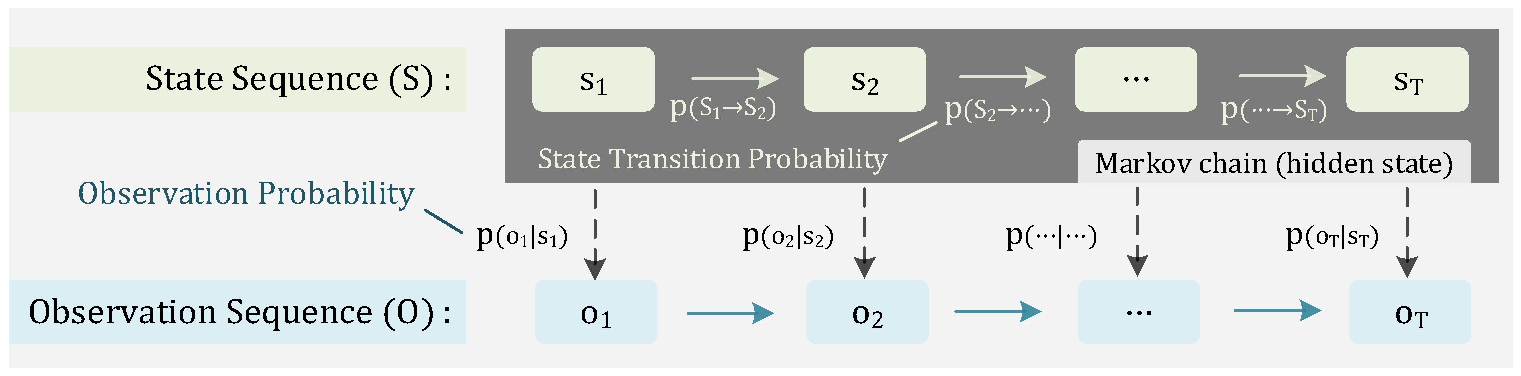
The Hidden Markov Model (HMM) is a statistical analysis model that describes a double stochastic process, including the hidden state transition process (Markov chain) and the observation process produced by specific states. Figure 1 shows the Hidden Markov process.

Let Q and V denote the state and observation spaces, which can be expressed as follows:

$$\left\{\begin{array}{l}Q=\left\{q_1,q_2,\dots ,q_N\right\}\\ V=\left\{v_1,v_2,\dots ,v_M\right\}\end{array}\right.$$

(1)

where N and M are the numbers of all possible states and observations. The HMM can be described as follows:

$$\lambda =\left(A,B,\pi \right)$$

(2)

where A denotes the state transition probability matrix, which can be described as follows:

$$A={\left[a_{ij}\right]}_{N\times N}$$

(3)

where a_ij represents the probability of transitioning to state q_j at time t + 1 when in the state q_i at time t, which can be expressed as follows:

$$a_{ij}=P(s_{t+1}=q_j|s_t=q_i),i=j=1,2,\dots ,N$$

(4)

B denotes the observation probability matrix:

$$B={[b_i(k)]}_{N\times M}$$

(5)

where b_i(k) represents the probability of generating observation v_k in state q_i at time t, which can be expressed as follows:

$$b_i(k)=P(o_t=v_k|s_t=q_i),i=1,2,\dots ,N;k=1,2,\dots ,M$$

(6)

π is the initial state probability vector:

$$\pi ={[{\pi }_i]}_N$$

(7)

where π_i is the probability of being in the state i, which can be expressed as follows:

$${\pi }_i=P(s_t=q_i),i=1,2,\dots ,N$$

(8)

HMM provides solutions to the following three basic problems. First, given the observation sequence O and the model λ, how to calculate the probability P(O|λ), namely the evaluation problem. Second, the learning problem is how to estimate the model parameters through the given O to maximize the probability P(O|λ). The last, given the observation sequence O and the model λ, is how to find the most likely hidden state S, namely the decoding problem.

The backward-forward algorithm is used to solve the evaluation problem, which also plays a core role in the approximation algorithm for the decoding problem. The learning problem can be solved by the maximum likelihood estimation (MLE) and the Baum–Welch algorithm. The approximation algorithm and the Viterbi algorithm can be used to solve the decoding problem. More details on applications of these algorithms in HMM can be found in the articles of Rabiner et al.

2.2. Multi-Observation Non-Homogeneous Hidden Markov Model

In this subsection, the traditional HMM is expanded on its two basic assumptions: first is the homogeneous Markov assumption, which means the state at any time is only related to the previous state and has nothing to do with the states and observations at other times. The homogeneous Markov assumption can be expressed as follows:

$$P\left(s_t|s_{t-1},o_{t-1},s_{t-2},o_{t-2}\dots ,s_1,o_1\right)=P\left(s_t|s_{t-1}\right)$$

(9)

Second is the observation independence assumption, which assumes that the observation at any time only depends on the state of the Markov chain at the same time, and has nothing to do with other observations and states. The observation independence assumption can be expressed as follows:

$$P\left(o_{t+1}|s_T,o_T,\dots ,s_t,o_t,\dots ,s_1,o_1\right)=P\left(o_{t+1}|s_{t+1}\right)$$

(10)

By analogy with the definition of Markov chain, traditional Markov chains can be extended to τ-order memory Markov chains, which means the conditional probability distribution of the future state depends on the past τ states, i.e.,

$$P\left(s_{t+1}|s_t,o_t,s_{t-1},o_{t-1}\dots ,s_1,o_1\right)=P\left(s_{t+1}|s_t,s_{t-1},\dots ,s_{t-\tau }\right)$$

(11)

Assuming that the observation at any moment depends not only on the hidden state at that moment but also on the previous observations or even the previous state, which can be described as follows:

$$P\left(o_{t+1}|s_T,o_T,\dots ,s_t,o_t,\dots ,s_1,o_1\right)=P\left(o_{t+1}|s_{t+1},s_t,o_t,\dots ,s_{t-n},o_{t-m}\right)$$

(12)

where n and m denote the orders of dependence on states and observations.

In practice, it is possible for each state to produce two or more observations. The introduction of multiple observations has the potential to improve the description accuracy. The multiple observation spaces and sequences can be described as follows:

$$\left\{\begin{array}{c}{V}^{(d)}=\left\{v_1^{(d)},v_2^{(d)},\dots ,v_M^{(d)}\right\}\\ O^{(d)}=\left\{o_1^{(d)},o_2^{(d)},\dots ,o_T^{(d)}\right\}\end{array}\right.$$

(13)

where d is the number of the observation type, which is a positive integer.

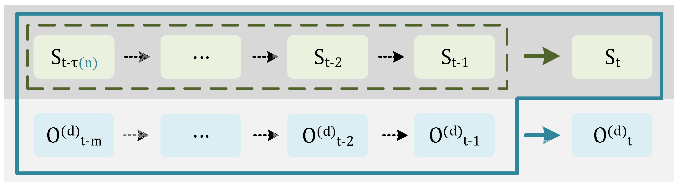
Figure 2 intuitively illustrates the interaction between the extended state and observation dependencies. The upper part shows the hidden state sequence with τ-order memory, while the lower part highlights the corresponding multi-type observation sequences, each incorporating up to m historical observations. This diagram clearly represents how both past states and observations jointly influence the current output, emphasizing the extended temporal and multimodal structure of the proposed HMM.

2.3. Model Parameter Estimation

Model parameter estimation is essentially an HMM learning problem, which is usually solved by the MLE or Baum–Welch algorithm. Given the natural time scale characteristics of the solar power generation series, the MLE is used to estimate the parameters. For the traditional HMM, the estimation of the transition probability and observation probability can be obtained as follows:

$$\left\{\begin{array}{l}{\widehat{a}}_{ij}={\displaystyle \frac{n_{ij}}{{\displaystyle \sum _{j=1}^N{n}_{ij}}}},i=j=1,2,\dots ,N\\ {\widehat{b}}_i(k)={\displaystyle \frac{n_{ik}}{{\displaystyle \sum _{k=1}^M{n}_{ik}}}},k=1,2,\dots ,M\end{array}\right.$$

(14)

where n_ij refers to the number of transitions from state i to state j in the training data; n_ik represents the number of times observation symbol k is generated from state i in the training data.

The extended HMMs, denoted by τ × n × m-MOHMM, can be estimated by

$$\left\{\begin{array}{l}{\widehat{a}}_{I^{(\tau )}j}={\displaystyle \frac{n_{I^{(\tau )}j}}{{\displaystyle \sum _{j=1}^N{n}_{I^{(\tau )}j}}}},I^{(\tau )}=\left\{i^1,i^2,\dots ,i^{\tau }\right\},j=1,2,\dots ,N\\ {\widehat{b}}_{I^{(n)}{W}^{(m)}}^{(d)}(k)={\displaystyle \frac{n_{I^{(n)}{W}^{(m)}k}^{(d)}}{{\displaystyle \sum _{k=1}^M{n}_{I^{(n)}{W}^{(m)}k}^{(d)}}}},W^{(m)}=\left\{w^1,w^2,\dots ,w^m\right\},k=1,2,\dots ,M\end{array}\right.$$

(15)

where I and W are the sequences of past state and observation; ${\widehat{a}}_{I^{(\tau )}j}$ refers to the estimated transition probability from a τ-length historical hidden state sequence $I^{(\tau )}$ to the current state j; $n_{I^{(\tau )}j}$ is the number of times that the sequence $I^{(\tau )}$ is followed by state j in the training data; ${\widehat{b}}_{I^{(n)}{W}^{(m)}}^{(d)}(k)$ refers to the estimated emission probability of observing symbol k in observation d, conditioned on: $I^{(n)}$ a n-length historical state sequence $\left\{i^1,i^2,\dots ,i^n\right\}$; $W^{(m)}$ an m-length historical observation sequence $\left\{w^1,w^2,\dots ,w^m\right\}$. $n_{I^{(n)}{W}^{(m)}k}^{(d)}$ refers to the number of occurrences of symbol k (in observation d) associated with history ($I^{(n)},W^{(m)}$); M is the number of discrete observation symbols per modality.

2.4. Decoding Problem

The decoding or forecast problem is that given the observation sequences, calculating the most likely corresponding state sequence. As mentioned in Section 2.1, the approximation algorithm and the Viterbi algorithm are two effective solutions, which are described in detail in the literature by Rabiner et al. [24,25,26]. In this section, the forward-backward algorithm for the decoding process of the τ × n × m-MOHMM is proposed.

Given the model λ and observation sequences O(d), the forward and backward probabilities can be expressed, respectively, as follows:

$$\left\{\begin{array}{l}{\alpha }_t\left(i_{\tau -1}\dots i_{1}j\right)=P\left(o_1^{(d)}\dots o_t^{(d)},s_{t-(\tau -1)}=q_{i_{\tau -1}},\dots ,s_{t-1}=q_{i_1},s_t=q_j | \lambda \right)\\ {\beta }_t\left(i_{\tau -1}\dots i_{1}j\right)=P\left(o_{t+1}^{(d)}\dots o_T^{(d)},s_{t-(\tau -1)}=q_{i_{\tau -1}},\dots ,s_{t-1}=q_{i_1},s_t=q_j | \lambda \right)\end{array}\right.$$

(16)

And it can be calculated iteratively according to the following steps. First of all, the initial values need to be calculated:

$$\left\{\begin{array}{l}{\alpha }_{\tau }\left(i_{\tau -1}\dots i_{1}j\right)={\pi }_{i_1}{\displaystyle \prod _{z=1}^d{b}_{i_{\tau -1}}^{(z)}\left[o_1^{(z)}\right]\dots a_{i_{\tau -1}\dots i_1}{\displaystyle \prod _{z=1}^d{b}_{\left(i_n\dots i_1\right)\left[o_{\tau -m}^{(z)}\dots o_{\tau -2}^{(z)}\right]}^{(z)}\left[o_{\tau -1}^{(z)}\right]a_{i_{\tau -1}\dots i_{1}j}{\displaystyle \prod _{z=1}^d{b}_{\left(i_{n-1}\dots i_{1}j\right)\left[o_{\tau -m}^{(z)}\dots o_{\tau -1}^{(z)}\right]}^{(z)}\left[o_{\tau }^{(z)}\right]}}}\\ {\beta }_T\left(i_1\dots i_{\tau -1}j\right)=1\end{array}\right.$$

(17)

Then, the forward-backward probability can be obtained by the following recursion formula:

$$\left\{\begin{array}{l}{\alpha }_{t+1}\left(i_{\tau -2}\dots i_{1}jk\right)=\left[{\displaystyle \sum _{i_{\tau -1}=1}^N{\alpha }_t\left(i_{\tau -1}\dots i_{1}j\right)}{a}_{i_{\tau -1}\dots i_{1}jk}\right]{\displaystyle \prod _{z=1}^d{b}_{\left(i_{n-2}\dots i_{1}jk\right)\left[o_{t-(m-1)}^{(z)}\dots o_t^{(z)}\right]}^{(z)}\left[o_{t+1}^{(z)}\right]},t=\tau ,\tau -1,\dots ,T-1\\ {\beta }_t\left(i_{\tau -1}\dots i_{1}j\right)={\displaystyle \sum _{k=1}^N{a}_{i_{\tau -1}\dots i_{1}jk}{\displaystyle \prod _{z=1}^d{b}_{\left(i_{n-2}\dots i_{1}jk\right)\left[o_{t-(m-1)}^{(z)}\dots o_t^{(z)}\right]}^{(z)}\left[o_{t+1}^{(z)}\right]}}{\beta }_{t+1}\left(i_{\tau -2}\dots i_{1}jk\right),t=T-1,\dots ,\tau -1,\tau \end{array}\right.$$

(18)

where ${\alpha }_{t+1}\left(i_{\tau -2}\dots i_{1}jk\right)$ is the forward probability of the joint probability of observing the first t + 1 observation vectors and ending in the state sequence $\left\{i_{\tau -2}\dots i_{1}jk\right\}$ at time t + 1; ${\beta }_t\left(i_{\tau -1}\dots i_{1}j\right)$ is the backward probability: the probability of future observations (from t + 1 to T) given the current state sequence $\left\{i_{\tau -1}\dots i_{1}j\right\}$ at time t; $a_{i_{\tau -1}\dots i_{1}jk}$ denotes the transition probability from the past τ-length state sequence $\left\{i_{\tau -1}\dots i_{1}j\right\}$ to next state k; $b_{\left(i_{n-2}\dots i_{1}jk\right)\left[o_{t-(m-1)}^{(z)}\dots o_t^{(z)}\right]}^{(z)}$ is the emission (observation) probability function for observation z, conditioned on the history of hidden states and past observations; $o_t^{(z)}$ is the observed state from the z-th observation at time t.

Then, the probability of being in state q_i at time t can be calculated as follows:

$${\gamma }_t\left(j\right)={\displaystyle \frac{{\displaystyle \sum _{i_{\tau -1}=1}^N\dots {\displaystyle \sum _{i_2=1}^N{\displaystyle \sum _{i_1=1}^N{\alpha }_t\left(i_{\tau -1}\dots i_{1}j\right){\beta }_t\left(i_{\tau -1}\dots i_{1}j\right)}}}}{P\left(O | \lambda \right)}}$$

(19)

which gives the probability distribution of the state at time t. The probability of the O(d) can be calculated as follows:

$$P\left(O|\lambda \right)={\displaystyle \sum _{i_{\tau -1}=1}^N\dots {\displaystyle \sum _{i_2=1}^N{\displaystyle \sum _{i_1=1}^N{\displaystyle \sum _{j=1}^N{\alpha }_t\left(i_{\tau -1}\dots i_{1}j\right){\beta }_t\left(i_{\tau -1}\dots i_{1}j\right)}}}}$$

(20)

And the most likely state at time t can be obtained as follows:

$$i_t^{*}=\arg \underset{1\le i\le N}{\max }\left[{\gamma }_t\left(i\right)\right],t=\tau ,\tau +1,\dots ,T$$

(21)

2.5. Power Predictor Modeling

During the actual operation, the power generation sequence is composed of power with a continuous and equispaced interval Δt, and so are the meteorological variables in NWP (maybe in a different interval). In this context, the power generation can be regarded as a hidden Markov process, and the meteorological parameters are the multiple observations. Then, the training and prediction functions of the prediction model can be completed by solving the learning and decoding problem of the HMM.

The power generation and meteorology sequences need to be discretized by defining several finite sets of values to formulate the prediction model. The state space is obtained by classifying the power generation level of the photovoltaic power station. For a specific PV station or distributed PV site, the range of corresponding stat space can be defined as [0, P_n], where P_n denotes the nominal power. Then, the set is obtained by θ, which classifies the power generation by the percentage interval of θ × P_n.

Similarly, let R_n refer to the maximum value of the d-th observation; the range of the corresponding observation space is [0, R_n], and the percentage interval is μ × R_n. Note that both θ and μ are defined as fractional values in the range [0, 1], representing the percentage intervals of the total range. The values of θ and μ are determined based on the input data resolution, signal variability, and the available training data volume. Finer discretisation increases the state-observation space dimensionality and requires significantly more data to avoid overfitting. Conversely, overly coarse discretisation can lead to information loss and reduced prediction accuracy. In this study, θ = 0.1 and μ = 0.1 are selected to achieve a practical balance between granularity and statistical robustness. The state and observation spaces can be described as follows:

$$\left\{\begin{array}{l}Q=\left\{0,q_2,\dots ,q_{N-1},P_n\right\}\\ V=\left\{0,v_2,\dots ,v_{M-1},R_n\right\}\end{array}\right.$$

(22)

where the number of discrete state levels N and observation levels M can be computed as N = 1/θ + 1 and M = 1/μ + 1, respectively.

3. Probability Distribution Estimation

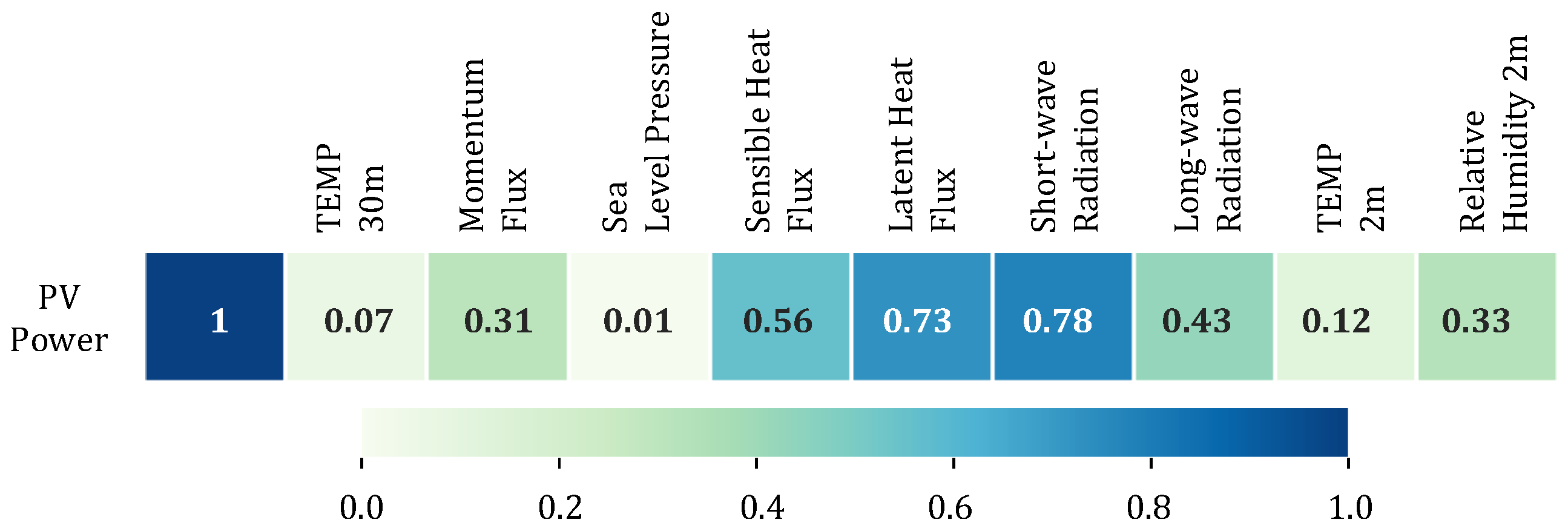
The research in this paper is based on a dataset, which is collected from a real-world grid-connected photovoltaic power plant located in a typical mid-latitude region in East Asia. It spans from 1 January 2020 to 31 December 2021, with a temporal resolution of 15 min, including the measured photovoltaic power generation and the corresponding numerical weather forecast (NWP). Preprocessing involved aligning timestamps, linear interpolation for missing values shorter than 1 h, discarding longer gaps, and smoothing outliers detected using a 3σ threshold. Figure 3 shows that the short-wave radiation has the highest correlation with PV power generation, followed by the latent heat flux with a coefficient value of 0.73. In light of this, these two parameters are selected as observations in the proposed extended HMMs.

The proposed probabilistic forecast models allow for the direct obtaining of the probability estimate (i.e., the state transition probability and observation probability) based on the past real solar power data. For example, Figure 3 shows the diagram of the state transition probability and observation probability of the PFM based on the traditional HMM with two observations. The state transition probability diagram describes the probability of s(t) at time t transitioning to s(t + 1) at time t + 1. It can be seen that the probability of transition between adjacent states is relatively large; only a few states with large spans have mutual transitions with a low probability, which is consistent with the practical situation.

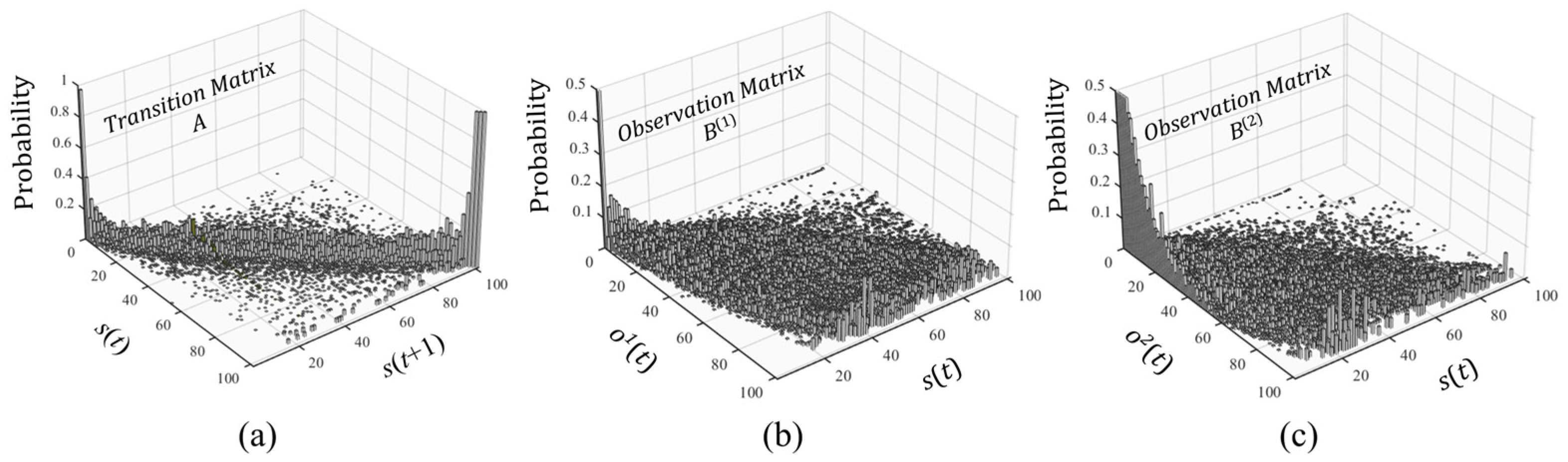
Figure 4 illustrates the estimated transition and observation probability distributions derived from the proposed extended HMM. Figure 4a shows the transition probability matrix, which captures the likelihood of moving from s(t) to s(t + 1). Figure 4b,c shows the observation probability matrices for two types of observed variables (e.g., solar irradiance and latent heat flux). It can be observed that the transition probabilities are concentrated along the diagonal of the matrix and gradually decay inward from both sides of the diagonal, indicating that the stepwise variation in output data aligns with a continuous-time physical process approximation. The observation probability diagram describes the probability of the state being s(t) when observation is o(t) at time t. It is worth noting that the observation probability is more dispersed compared to the transition probability. In other words, at a certain moment, a state corresponds to a larger number of observations at a higher probability level.

After obtaining the transition and observation probability matrices, the state probability distribution at each time step can be derived by solving the decoding problem. Utilizing the probability matrices shown in Figure 4 along with the NWP data, the probabilistic distribution of PV power generation is estimated for each time step over the next three days, with a temporal resolution of 15 min. Furthermore, the resulting probability distributions can serve as the basis for constructing both point forecasts and interval predictions, thereby enhancing the robustness and flexibility of the framework. For the point predictor, it can be obtained by the mean:

$$s{(t)}_{Mean}={\displaystyle {\sum }_{i=1}^N{s}_i{\gamma }_t(i)}$$

(23)

or mode

$$s{(t)}_{Mode}=s_j:\underset{i=1,2,\dots ,N}{\max }\left[{\gamma }_t(i)\right]={\gamma }_t(j)$$

(24)

Given a quantile parameter α, the PIs can be obtained by the following:

$$s{(t)}_{\alpha }=s_j:\left\{\begin{array}{l}{\displaystyle {\sum }_{i=1}^j{\gamma }_t(i)\ge \alpha }\\ {\displaystyle {\sum }_{i=1}^{j-1}{\gamma }_t(i)<\alpha }\end{array}\right.,0<\alpha <1$$

(25)

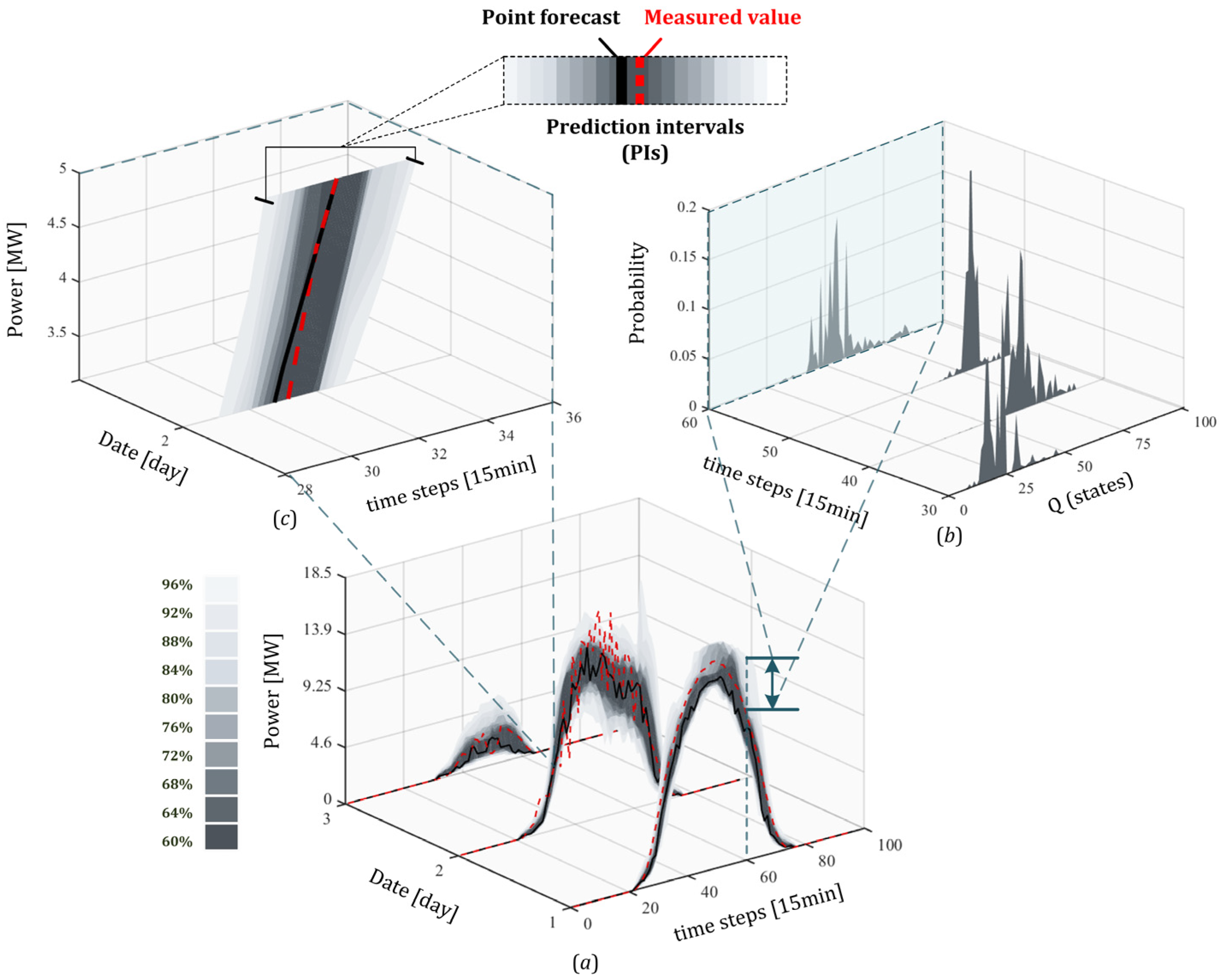
Figure 5 presents a comprehensive illustration of how point forecasts and probabilistic forecasts are derived from the extended Hidden Markov Model (HMM). Figure 5a shows the predicted PV power output over a 3-day period, with point forecasts in black, measured values in red, and shaded prediction intervals (PIs) at multiple confidence levels. The forecasted power output closely follows the actual measurements, and the majority of true values fall within the shaded prediction intervals, especially around peak hours, indicating good calibration of the forecast uncertainty. Figure 5b is the top-right subplot, which depicts the posterior distribution of hidden states over time, illustrating how the model captures uncertainty in the underlying regime. The state posterior distributions are temporally adaptive—the model assigns higher confidence to certain states during stable periods (e.g., early morning and evening), while distributing probability more broadly during midday when solar variability increases. Figure 5c is the zoomed-in panel (left), which magnifies a selected time window, clearly showing the structure and width of the prediction intervals around the forecast curve. Together, these subplots demonstrate how the model quantifies uncertainty at both the output and hidden state levels, thereby supporting both deterministic forecasting and probabilistic decision-making.

4. Model Analysis

In this section, the performance of the models that are based on Markov chains of different orders and the degree of correlation with the observation information (i.e., the parameters τ, n, and m in the extended HMM) are analyzed in detail. Model evaluations are performed using cross-validation over a two-year dataset, covering diverse seasonal and meteorological conditions. This effectively tests the model’s robustness across different operational scenarios.

Table 1. The information about the proposed models.

Model Number	1	2	3	4	5	6	7	8	9	10	11	12	13
d	1	2	2	2	2	2	2	2	2	2	2	2	2
τ	1	1	1	1	1	1	1	2	2	2	2	2	2
n	1	1	1	1	2	2	2	1	1	1	2	2	2
m	0	0	1	2	0	1	2	0	1	2	0	1	2

summarizes the structural configurations of the proposed models used for performance evaluation in the extended HMM framework. Each column represents a specific model, characterized by four key parameters. The table illustrates how individual models differ in complexity and temporal correlation structure. For example, Model 1 is the simplest configuration, with a single observation type and first-order Markov assumptions, corresponding to a traditional first-order HMM. In contrast, Model 13 is among the most complex, incorporating two observation types and second-order dependencies across all parameters. By systematically varying these parameters across the models, the study enables a comprehensive analysis of how memory depth and observation coupling influence forecasting performance in the extended HMM framework.

The remaining probabilistic forecasting models were constructed by relaxing the two aforementioned assumptions. This section conducts a series of crossover experiments for each model following the steps below. First, three days of data are randomly selected as the test set, while the remaining data are used for model parameter estimation. The trained model is then employed to generate point forecasts and prediction intervals. Subsequently, the evaluation metrics are computed and recorded. This procedure is repeated until a total of 1000 iterations is completed. It is observed that as the number of iterations approaches 1000, the distributions of the evaluation metrics converge and exhibit stability. The statistical results of the PIs and point forecast metrics across all models are presented in Figure 6 and Figure 7, respectively.

For point forecast results, the normalized root mean square error (NRMSE) is used as the metric. NRMSE provides a scale-independent measure of prediction deviation by normalizing RMSE against the data range, making it suitable for comparing models across different magnitudes. As shown in Figure 6, which presents a statistical distribution (via violin plots) of the NRMSE values across 13 MOHMM variants, Model 4 and Model 9 exhibit lower and more stable errors.

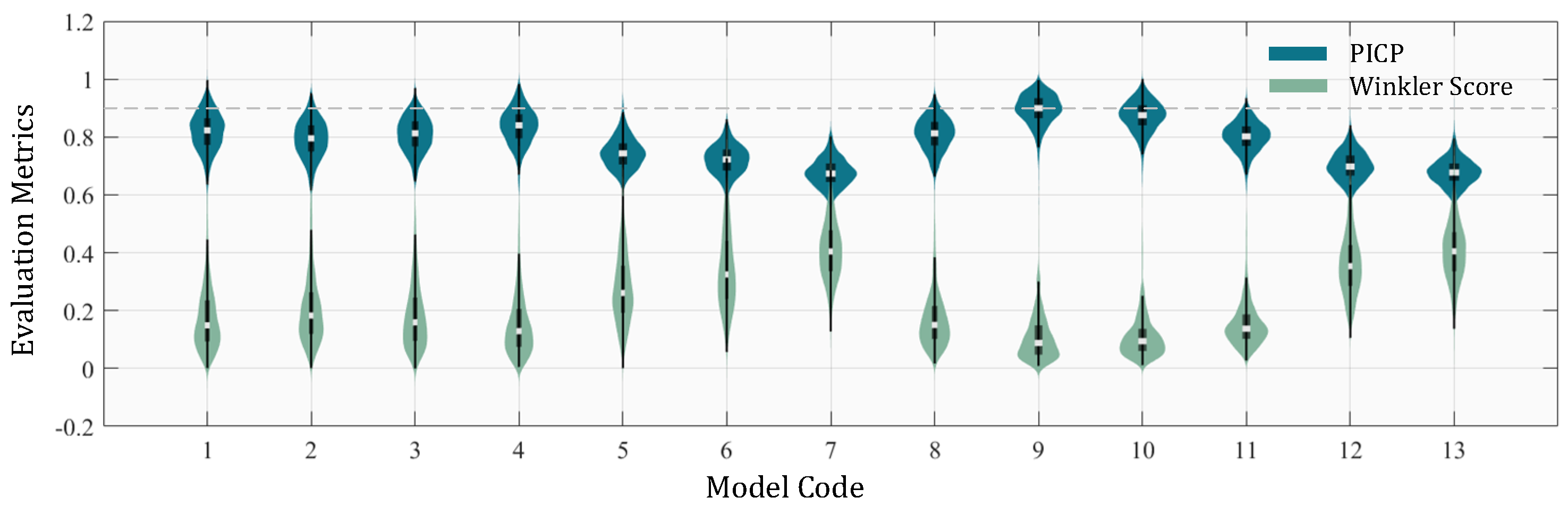
For the PIs, prediction interval coverage probability (PICP) and Winkler score, respectively, characterize the performance of the model in terms of reliability and sharpness. PICP (Prediction Interval Coverage Probability) measures the proportion of true values falling within a given prediction interval (e.g., 90%). Winkler Score combines both the width of prediction intervals and penalties for coverage misses, offering a balanced measure of sharpness and reliability. It can be seen in Figure 7 that, similar to point prediction, models 4, 9, and 10 also show good performance in the PIs, while models 6, 7, 12, and 13 have the worst. A slight difference is that models 9 and 10 have better scores than model 4 in both reliability and sharpness of the PIs. This indicates that considering the influence of past observation information and state on the current observation can effectively improve the prediction performance of the model. However, consideration of excess information from past observations can lead to a significant reduction in model performance, as presented by models 6, 7, 12, and 13.

After identifying the best-performing MOHMM configuration (model 9, d = 2, τ = 2, n = 1, m = 11), we further evaluated its performance against several widely used probabilistic forecasting models, namely quantile regression forests (QRF), Bayesian neural networks (BNN), and LightGBM with quantile objective (LightGBM-QR). These models were selected due to their proven effectiveness in time series regression and uncertainty quantification. All baseline models are trained using the same input features and training/testing protocol as the proposed method.

The results are summarized in

Table 2. Performance comparison of MOHMM and baseline probabilistic forecasting models.

Model	Winkler Score	PICP	RMSE	Interpretability	Training Time
MOHMM	0.109	91.2%	0.144	High	Low
QRF	0.119	90.5%	0.150	Medium	Low
BNN	0.126	89.7%	0.147	Low	High
LightGBM-QR	0.115	91.0%	0.143	Medium	Low

. As shown, the proposed MOHMM achieves the best overall performance in probabilistic forecasting. It obtains the lowest Winkler score (0.109), indicating sharper and more calibrated prediction intervals, and achieves the highest PICP (91.2%), suggesting strong reliability in uncertainty quantification. Its RMSE is comparable to the best-performing method (LightGBM-QR), but with significantly higher interpretability.

QRF offers reasonably good interval coverage and low RMSE but lacks a mechanism to model temporal dependencies or latent state transitions, which are critical in sequential energy forecasting tasks. BNN is theoretically powerful but suffers from training instability, high computational cost, and low interpretability, making it less suitable for real-time or embedded applications. LightGBM-QR delivers high accuracy and fast training, but like QRF, it treats each prediction independently and does not offer insight into temporal regime shifts or underlying stochastic patterns. In contrast, MOHMM provides a transparent probabilistic model that not only captures the predictive distribution effectively but also reveals the evolving internal structure of power generation dynamics via its hidden state transitions. These advantages make MOHMM a compelling choice for real-world deployment, especially in resource-constrained or explainability-critical scenarios such as energy scheduling and grid control.

5. Conclusions

Based on the Hidden Markov Model (HMM), this study proposes a probabilistic forecasting model (PFM) for solar power by discretizing PV output and associated meteorological features into intensity levels, which define the state and observation spaces. Transition and observation probability matrices are estimated from real-world PV system operation data, and the decoding process yields time-resolved probability density distributions. To enhance forecasting capability, the classical HMM is further extended to incorporate non-homogeneous structures and observation dependencies, resulting in 13 model variants that are comprehensively evaluated in terms of point forecasts and prediction intervals (PIs). The results demonstrate that, under a 15 min forecasting resolution, incorporating dependencies on both historical states and observations significantly enhances model performance. Specifically, models utilizing second-order observation dependencies outperform their first-order counterparts in terms of PI accuracy. However, introducing second-order state dependencies adversely affects performance, suggesting that excessive reliance on historical state information can introduce redundancy and degrade prediction quality. This finding aligns with practical insights: while recent observation data (e.g., from the past 30 min) show strong correlation with current states and outputs, earlier state information (e.g., PV power history) may contain redundant or less informative content, ultimately increasing model error.

This paper provides a detailed derivation and demonstration of the development and extension of a statistically grounded PFM for solar forecasting. As an initial exploration into practical applications, several aspects merit further investigation. These include the impact of discretization parameters (e.g., μ and θ) on model accuracy, and the trade-off between dataset size and model complexity. Addressing these factors will be critical for tailoring the proposed framework to diverse operational scenarios and ensuring its robustness in broader energy forecasting contexts.

Future research will focus on further enhancing the adaptability and scalability of the proposed method. Potential directions include: (1) incorporating online learning mechanisms to dynamically adjust model parameters in real-time; (2) fusing multimodal data such as weather forecasts, market information, and sensor signals to enrich input representations; and (3) extending the framework to regional multi-energy systems for coordinated probabilistic scheduling and control.