Heat-Loss Based Method for Real-Time Monitoring Method for Hydroelectric Power Plant Efficiency

Abstract

In energy transition scenarios, hydropower remains the largest source of renewable electricity generation. However, with respect to other means of renewable energy exploitation, like wind turbines or photovoltaics, very few technological advancements are to be expected, due to the technological maturity of hydropower turbines. Therefore, an increase in power production of hydropower plants can only be possible thanks to an optimization of the operation and maintenance policies, leading to improved performance, reducing energy losses and downtimes. This work proposes a practical approach to the continuous monitoring of the operational conditions of hydropower plants through the non-invasive measurement of the electrical efficiency of the generator group. To achieve this, a heat-loss based method is introduced, which enables the measurement of both the electrical generator losses and the electrical input power, along with their associated uncertainties. This method is applicable for plants of any size, does not require a production shutdown, and, since it is applied to the electrical generator, can be used with different turbine types, including Kaplan, Francis, and Pelton. It also relies on relatively simple instruments such as thermo-cameras, thermo-resistances, thermo-couples, and flow meters to measure key variables, including cooling water inlet and outlet temperatures, electrical machine external and frame temperatures, undisturbed ambient temperature, electrical power absorbed, and cooling water flow rate. The proposed methodology has been tested and validated through the application to a laboratory test rig. In all test conditions, the heat loss-based method showed a smaller relative error than the standard efficiency measurement methods.

1. Introduction

Hydropower has always been the predominant source of renewable energy generation, currently exceeding 1400 GW of installed capacity worldwide [1]. However, the already-established role of hydropower in the energy mix is become even more crucial with the increased penetration of fast-variable renewable energy sources, such as photovoltaics and wind [2]. In fact, the flexibility of hydropower can mitigate the fluctuations induced by temporal variations in solar and wind resources, effectively contributing to overall net stability [3].

In addition, the targets set by the 2030 net-zero scenario require a growth in hydropower capacity at a rate of 26 GW per year. New installations are expected to mostly occur in developing countries, although factors such as complex permitting policies and weak investor participation are partially hampering their growth.

The upcoming additions to installed capacity, along with the repowering of existing hydroelectric power plants (HPPs), advocate novel methods to improve plant reliability, support operation and maintenance policies, and monitor the health status of the systems [4]. These aspects are particularly relevant in medium- and large-sized HPPs that undergo continuous operations, where even limited and partial shutdowns may result in significant economic losses. One of the key parameters to measure the system’s status is the global efficiency of the HPP, which encompasses the efficiency of each main component of the conversion process (e.g., mechanical, electrical, and hydraulic efficiency).

In accordance with national and international standards, such as the Italian CEI 60041 [5], the overall efficiency computation is performed using a purely energy criterion, measuring the ratio between the available energy at the inlet and the power output of the HPP. However, efficiency measurement requires the acquisition of physical quantities at different locations of the system, obtained through a long and expensive on-field campaign, using an acquisition system specifically designed for the plant’s size and layout. As a result, the efficiency measurement of HPPs is limited to an intermittent monitoring performed every few years.

Recent advancements in efficiency measurement techniques aim to address the challenges posed by intermittent monitoring and the high costs of traditional on-field campaigns. Several studies have proposed methods to overcome these challenges by combining new technologies, such as remote sensing and computational approaches, for more effective efficiency monitoring of HPPs [6,7,8]. These innovations enable more frequent and cost-effective assessments, reducing reliance on plant-specific setups.

Additionally, several studies shift their focus to the efficiency considerations of individual components, such as turbines [9,10,11], generators [12,13], penstock [14,15] and transformers [16]. This component-centered approach, as observed by Yang et al. [17], facilitates a more effective monitoring of efficiency and contributes to reducing operational downtime.

Emerging trends also highlight the integration of predictive maintenance systems [18] and real-time monitoring tools [19] to enhance overall efficiency measurement. These innovations leverage IoT-enabled sensors [20,21] and advanced data analytic [22] to continuously monitor key performance metrics, allowing operators to proactively detect inefficiencies or potential failures. Such technologies are particularly advantageous for the medium- and large-sized HPPs discussed [23], as operational disruptions in these systems can lead to significant economic losses [24,25]. However, it must be considered that some of these technological arrangements are only feasible during the installation stage of the plants, while others require substantial investment that may not be economical, especially for existing HPPs [26].

This work proposes a novel approach for the computation of electrical efficiency, hereby referred to as the heat loss-based method, based on the application of the energy conservation law. Specifically, losses in the generators correspond to an increase in the temperature of the cooling fluid and/or generator surfaces, which can be measured non-invasively and using cost-effective instruments. The comparison with nameplate conditions immediately highlights the health status of these components and provides warnings about incipient or existing failures. Since the electrical group represents one of the major sources of losses and failures in an HPP, the proposed approach could effectively reduce plant downtime and support maintenance policies. However, it should be noted that the heat loss-based method does not constitute an alternative to traditional, regulated methods but is instead designed as an auxiliary monitoring system.

This approach can be considered novel and distinct from the traditional calorimetric method because: (a) it is applied to the cooling fluid of the electrical group of a hydroelectric power plant (HPP), rather than to the turbine core flow; (b) it accounts for the majority of thermal losses, including those occurring through convection and radiation; and (c) it can be used to detect failing or off-design operation in various components of the HPP.

As such, this approach overcomes the well-known limitations of standard thermodynamic methods, which are difficult to apply when the turbine’s rated power falls below 5 MW, due to the negligible rise in water temperature under such conditions. Since this method relies solely on temperature probes, a fluxmeter, and a thermal camera (the latter is only required in Configuration A), it can be considered cost-effective. In contrast, the typical procedure for testing turbine performance often requires the plant to shut down for several days in order to install volumetric flow and pressure measurement devices at the turbine discharge. With the proposed method, only the generator losses are monitored, and the necessary modifications to the plant—such as clamp-on fluxmeters and inlet/outlet water thermocouples—are installed only once.

The paper is structured as follows. Section 2 presents the theoretical formulation of the heat loss-based method, applied to two possible configurations of electrical motors, and further details the derivation of the associated uncertainties. Section 3 describes the experimental and measurement apparatus, as well as a possible application of the methodology to a real HPP. This is followed by Section 4 including a comparison between the two configurations and the efficiency calculations of an electrical motor. Additional notes on the configuration comparison are provided in the annex. Finally, Section 5 summarizes the main findings of the study.

2. Heat Loss-Based Method

This section describes the development of a calorimetric method for measuring power loss in a liquid-cooled electrical motor. Two configurations are analyzed to measure the electrical motor’s losses and input power, along with their uncertainties, that differs on the treatment of heat fluxes on the solid surfaces. A theoretical analysis outlines the Heat loss-based system’s features and forecasts expected results. This forecast is based on data from liquid-cooled motors rated up to 30 kW and similar studies from the literature [27]. This motor type was chosen to enable a comparison between the theoretical predictions and real data measured during test bench experiments.

2.1. Configuration A

In this configuration [28] shown in Figure 1, heat losses are calculated by defining an additional boundary around the motor surface as the control volume. This boundary is introduced to account for the portion of heat loss emitted directly into the environment from the surface of the motor, which is otherwise difficult to measure. The boundary consists of an insulation housing with an internal polystyrene frame and an external wood frame, designed to isolate the motor from the environment and direct most heat through the motor’s cooling system. By measuring the volumetric flow rate of the cooling fluid and the temperature difference between its inlet and outlet, a significant portion of the power loss can be accurately determined [29].

Before obtaining reliable power loss values, the motor and insulation box must reach the steady-state temperature, which is determined by the specific operating conditions, including the operating point and the power lead away by the cooling system. Due to the motor’s thermal inertia, reaching thermal equilibrium takes time. According to CEI EN 60034, equilibrium is reached when temperature variations remain below 5 °C for 30 min, at which point the insulation box temperature stabilizes, and heat loss balances with the heat lead away by the cooling system [30].

The contribution of the losses can be inspected and analyzed separately.

2.1.1. Heat Transferred to the Water Cooling System

The heat dissipated in the water cooling system can be computed using Equation (1):

$$P_{\mathrm{wat},\mathrm{cool}}=\rho ·Q·c_p·(T_{\mathrm{wat},\mathrm{out}}-T_{\mathrm{wat},\mathrm{in}})=\rho ·Q·c_p·\Delta T$$

(1)

where $\rho$, Q, $c_p$, and $\Delta T$ are, respectively, the density, the volumetric flow rate, the specific heat capacity at constant pressure, and the temperature difference between the inlet and outlet of the cooling system. The volumetric flow rate Q used in this model is selected from the catalog of a 30 kW liquid-cooled motor, as listed in the Rowan Motor Catalog [31].

2.1.2. Heat Transmitted Through the Insulation Box

It can be evaluated through the following expression:

$$P_{\mathrm{ins},\mathrm{box}}=S_{\mathrm{ins},\mathrm{box}}·U_{\mathrm{tot}}·(T_{\mathrm{in},\mathrm{box}}-T_{\mathrm{out}})$$

(2)

where $S_{\mathrm{ins},\mathrm{box}}$ is the surface of the motor housing, $T_{\mathrm{in},\mathrm{box}}$ and $T_{\mathrm{out}}$ are, respectively, the air temperature inside and outside of the insulation box, and U is the thermal transmittance. The temperature outside the insulation box is fixed at the ambient temperature of 20 °C, while the inside temperature depends on the motor type and cooling system. An average temperature of 54 °C was adopted as the temperature inside the insulation box, based on experimental results from the literature [32], where a study used thermal imaging via optical fiber sensing and Raman scattering to analyze hydroelectric generator stator temperatures with a reduced 3D model.

Since thermal transmittance has an inverse relationship with thermal resistance, it is calculated using the following formula:

$$U_{tot}={\displaystyle \frac{1}{R_{int}+R_{wall}+R_{ext}}}$$

(3)

where $R_{\mathrm{int}}$ and $R_{\mathrm{ext}}$ are, respectively, the thermal resistances of the internal and external insulation layers, both accounting for convection and radiation, and $R_{\mathrm{wall}}$ is the thermal resistance of the insulating wall materials, accounting for conduction. Considering that convection and radiation mechanisms happen simultaneously, while conduction mechanisms take place consecutively, the thermal resistances are expressed as follows:

$$R_{int}={\displaystyle \frac{1}{h_{conv,int}+{\alpha }_{rad,int}}}$$

(4)

$$R_{ext}={\displaystyle \frac{1}{h_{conv,ext}+{\alpha }_{rad,ext}}}$$

(5)

$$R_{wall}={\displaystyle \frac{d_{int}}{{\lambda }_{int}}}+{\displaystyle \frac{d_{ext}}{{\lambda }_{ext}}}$$

(6)

In these equations, h denotes the convective heat transfer coefficient, while $\alpha$ represents the radiative heat transfer coefficient. The terms d and $\lambda$ correspond to the thickness and thermal conductivity of the layer, respectively. The subscripts int and ext indicate the internal and external layers. The surface temperatures of the internal and external layers are determined iteratively using an in-house code. These temperatures are then used to compute the mean temperatures of the layers, which serve as inputs for evaluating the radiative heat transfer coefficients ${\alpha }_{rad,int}$ and ${\alpha }_{rad,ext}$. The convective heat transfer coefficients used in this analysis are defined by the CEI EN 60034-2-2 standard [33].

2.1.3. Heat Flowing Through Gaps in the Insulation Layer

The convectional losses caused by the narrow gaps between individual polystyrene blocks are challenging to quantify. Heat loss-based tests have shown the presence of a vertical temperature gradient inside the box, which generates a small pressure difference between the interior and exterior. Further experiments and analyses specifically conducted to investigate this phenomenon revealed that the resulting volumetric flow rate accounts for approximately 3% of the heat flux led away in the cooling water circuit [27], such as the leakage losses can be estimated as:

$$P_{\mathrm{leakage}}=P_{\mathrm{wat},\mathrm{cool}}·0.03$$

(7)

2.1.4. Heat Lost by Shaft and Motor Frame (Convection and Radiation)

This loss includes both convection and radiation losses from the motor frame and the portion of the shaft within the control volume. This loss is expressed as follows:

$$P_{fr,\mathrm{conv}/\mathrm{rad}}=S_{fr}·\left(h_{\mathrm{conv}}+{\alpha }_{\mathrm{rad}}\right)·\left(T_{\mathrm{surf},fr}-T_{\mathrm{out}}\right)$$

(8)

Here, $S_{fr}$ is the surface area for convection and radiation, h—the convective coefficient, $\alpha$—the radiative coefficient, $T_{\mathrm{surf},fr}$—the surface temperature, and $T_{\mathrm{out}}$—the ambient temperature.

2.1.5. Heat Lost by Shaft and Motor Frame (Conduction)

Heat transfer by conduction depends on the material properties, temperature gradient, and geometry. For the shaft and motor frame, the total conductive heat loss is expressed as:

$$P_{fr,\mathrm{cond}}={\displaystyle \frac{S_{fr}·\lambda }{d}}·(T_{\mathrm{in}}-T_{\mathrm{out}})$$

(9)

Here, $S_{fr}$ is the conduction surface area, $\lambda$ the thermal conductivity, d the thickness of the motor frame or shaft, $T_{\mathrm{in}}$ the inside temperature, and $T_{\mathrm{out}}$ the outside (ambient) temperature.

2.1.6. Ventilation Losses

Forced air ventilation may be required if heat is not transferred fast enough to the cooling fluid, causing the air temperature to rise to unacceptable levels before the equilibrium is reached. In such cases, the power loss due to ventilation can be calculated by measuring the air’s volumetric flow rate and the temperature difference between the inlet and outlet. Since the fans used for ventilation also consume energy, their contribution must be included in the energy balance for heat loss-based measurements. This can be done by monitoring the DC voltage and current supplied to the fans.

$$P_{\mathrm{air},\mathrm{vent}}={\rho }_{\mathrm{air}}·Q_{\mathrm{air}}·c_{\mathrm{p}-\mathrm{air}}·(T_{\mathrm{air},\mathrm{out}}-T_{\mathrm{air},\mathrm{in}})$$

(10)

In summary, the total power loss $P_{\mathrm{loss}}$ consists of multiple components:

$$P_{\mathrm{loss}}=P_{\mathrm{wat},\mathrm{cool}}+P_{\mathrm{ins},\mathrm{box}}+P_{fr,\mathrm{conv}/\mathrm{rad}}+P_{fr,\mathrm{cond}}+P_{\mathrm{leakage}}+P_{\mathrm{air},\mathrm{vent}}$$

(11)

2.2. Configuration B

The relative error of Configuration A (Equation (30)) decreases to zero when its contribution to the total losses is small, such as the losses through the insulation box. Consequently, to avoid the challenges of constructing the insulation box, an alternative measurement method is used, as shown in Configuration B in Figure 2.

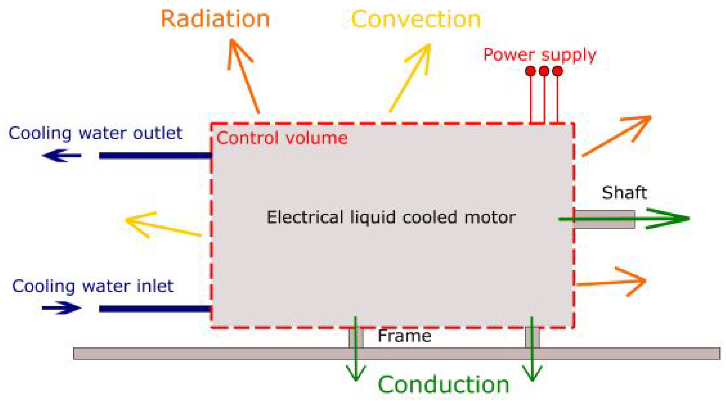
The principle is similar to Configuration A, but without the external box, convective and radiant losses are handled differently, with heat flux through the electrical machine’s wall estimated via a thermal camera. Estimating heat losses through the generation surface is more difficult in this configuration, making it less accurate. However, it can be a suitable method for electrical machines where constructing an insulation box is challenging, and where a cooling system minimizes heat flux through the external walls, ensuring effective heat removal. With a well-designed cooling system, it is expected to manage most of the heat transport, while the motor’s external surface and other loss sources contribute only a small amount. The ventilation losses are here neglected as the electrical machines are installed in open ambient. While the heat transferred to the water cooling system and the heat lost by the shaft and motor frame can be calculated similarly to Configuration A—i.e., according to Equations (1), (8) and (9), respectively—the modeling of the heat lost by the motor surface through convection and radiation must be modified. This is necessary since the insulation box is no longer present, and a direct exchange between motor surface with the surrounding ambient occurs.

The required measurements for this loss calculation are the external surface temperature and the undisturbed ambient temperature. The heat loss is determined by considering only the convective and radiant components.

$$P_{\mathrm{surf},\mathrm{motor}}=S_{\mathrm{motor}}·h_{\mathrm{conv}}·(T_{\mathrm{surf},\mathrm{ext}}-T_{out})+S_{\mathrm{motor}}·\sigma ·\epsilon ·(T_{\mathrm{surf},\mathrm{ext}}^4-T_{out}^4)$$

(12)

Here, $S_{\mathrm{motor}}$ is the motor’s external surface, h the convective coefficient, $\sigma$ the Stefan–Boltzmann constant, $\epsilon$ the emissivity, $T_{\mathrm{surf},\mathrm{ext}}$ the external surface temperature, and $T_{out}$ the undisturbed ambient temperature.

In summary, the total power loss in Configuration B consists of multiple components:

$$P_{\mathrm{loss}}=P_{\mathrm{wat},\mathrm{cool}}+P_{\mathrm{surf},\mathrm{motor}}+P_{fr,\mathrm{conv}/\mathrm{rad}}+P_{fr,\mathrm{cond}}$$

(13)

2.3. Uncertainty Analysis

According to UNI CEI EN 13005, measurement uncertainty is classified into two categories: A and B [34].

Type A standard uncertainty is determined through statistical analysis of a series of observations, resulting in a probability density function. To quantify this uncertainty, the mean value $\overline{y}$ of each data set is calculated as:

$$\overline{y}={\displaystyle \frac{1}{N}}\sum _{k=1}^N{y}_k$$

(14)

where N is the total number of measurements, and $y_k$ represents individual measurements. Random variations in $y_k$ arise from fluctuating influence factors, which cause the observations to differ. The experimental variance $s^2$ estimates the actual variance ${\sigma }^2$ of the probability distribution of y. This variance is calculated as:

$$s^2\left(y_k\right)={\displaystyle \frac{1}{N-1}}\sum _{k=1}^N{(y_k-\overline{y})}^2$$

(15)

This value reflects the dispersion of $y_k$ around the mean $\overline{y}$. The variance of the mean is then given by:

$$s^2\left(\overline{y}\right)={\displaystyle \frac{s^2\left(y_k\right)}{N}}$$

(16)

Finally, the Type A standard uncertainty for the mean is expressed as the positive square root of this variance:

$$\Delta y_A\left(\overline{y}\right)=s\left(\overline{y}\right)=\sqrt{s^2\left(\overline{y}\right)}$$

(17)

Type B standard uncertainty is evaluated when an estimate of a measurement is not obtained from repeated observations. It takes in account all available information about the variability of the measurement, including calibration certificates, technical specifications from the manufacturer, prior experience with the instrument, etc.

In this work, Type B uncertainty was determined using the uncertainties of the sensors and the data acquisition software employed for direct measurements. Specifically, uncertainties of the measuring instruments were derived from the manufacturer’s provided full-scale (FS) range and accuracy class. Since no background knowledge about the distribution of measurements provided by the manufacturer is available, a uniform probability distribution is assumed (Figure 3), where the semi-range limits $a^{-}$ and $a^{+}$ are provided by the manufacturer, and the range half-width is calculated as $a=0.5·\left(a^{+}+a^{-}\right)$. Standard uncertainty $\Delta y_B\left({\mu }_t\right)$, is then determined based on these assumptions as $\Delta y_B\left({\mu }_t\right)=a$.

Regarding the efficiency estimation, it cannot be measured directly and must be calculated from multiple individual measurements. Since errors in these individual measurements affect the final result, the combined standard uncertainty ($\Delta y$) quantifies how these errors propagate through the calculation. Consider a measurement model in the form of:

$$y=f(x_1,x_2,\dots ,x_n)$$

(18)

where, $x_1,x_2,\dots ,x_n$ are input variables, and y is the output quantity. The increments (absolute errors) of the inputs are denoted by $\Delta x_1,\Delta x_2,\dots ,\Delta x_n$. The combined standard uncertainty is expressed as:

$$\Delta y=f(x_1+\Delta x_1,x_2+\Delta x_2,\dots ,x_n+\Delta x_n)-f(x_1,x_2,\dots ,x_n)$$

(19)

Due to the computational costs associated with this direct computations, a simplified method based on the Taylor series expansion of the function $f(x_1,x_2,\dots ,x_n)$ around the actual (true conventional) values of the inputs is used. Neglecting higher-order terms, the combined standard uncertainty is approximated as:

$$\Delta y=\pm \sqrt{\sum _{i=1}^N{\left({\displaystyle \frac{\partial f}{\partial x_i}}\right)}^2·{(\Delta x_i)}^2}$$

(20)

This formula assumes independence of input quantities. If covariance terms are significant, they must also be included in the analysis. The combined standard uncertainty $u_c$ provides a realistic estimate of the result’s overall uncertainty, incorporating contributions from all inputs and their respective sensitivity coefficients.

For each physical quantity, the total standard uncertainty is calculated from the uncertainties of type A and B (combined or not):

$$y_{\mathrm{tot}}=\sqrt{y_A^2+y_B^2}$$

(21)

Building on this, we can now consider the uncertainty propagation in the efficiency of an electrical machine. The efficiency of a machine can be expressed as the ratio between useful power ($P_u$) and absorbed power ($P_a$) at the inlet:

$$\eta ={\displaystyle \frac{P_u}{P_a}}$$

(22)

This method of calculation is typically applicable to machines with lower power ratings (a few kVA). For instance, an electric machine with $P_a\approx 10\mathrm{kVA}$ generally has an efficiency ($\eta$) of about 0.85. In this case, a satisfactory efficiency value would be obtained if the uncertainty is less than 2% ($\Delta \eta \le 0.02$), with a relative error of approximately 2.35% (${\displaystyle \frac{\Delta \eta }{\eta }}=0.0235$).

To achieve this, it is essential that the starting uncertainties of the measurements of both the absorbed and useful power are sufficiently small. The maximum acceptable relative error in efficiency can be derived by differentiating the equation for efficiency:

$${\displaystyle \frac{\Delta \eta }{\eta }}=\sqrt{{\left({\displaystyle \frac{\Delta P_a}{P_a}}\right)}^2+{\left({\displaystyle \frac{\Delta P_u}{P_u}}\right)}^2}$$

(23)

Assuming high-quality instruments with a relative error of 1% (${\displaystyle \frac{\Delta P_a}{P_a}},{\displaystyle \frac{\Delta P_u}{P_u}}\approx 0.01$), the resulting relative error in efficiency is 1.41% (${\displaystyle \frac{\Delta \eta }{\eta }}=0.0141$), and the corresponding uncertainty becomes $\Delta \eta \approx 0.0120$. This provides a limit on the minimum accuracy required from the instruments. Consequently, the relative error in efficiency remains constant and depends solely on the uncertainty in the measurements of both the useful and absorbed power.

As an alternative, the efficiency of electrical machines involves measuring electrical power and machine losses, rather than directly measuring mechanical power at the shaft. This is beneficial because, for large machines, measuring torque and mechanical power can be difficult and requires costly equipment. In this method, the efficiency is calculated as:

$$\eta ={\displaystyle \frac{P_u}{P_u+P_{\mathrm{loss}}}}={\displaystyle \frac{P_a-P_{\mathrm{loss}}}{P_a}}$$

(24)

This approach, known as the conventional error method, leads to different error propagation characteristics compared to the standard method. The efficiency uncertainty, derived through error propagation analysis, is expressed as:

$$\Delta \eta =\pm \sqrt{\left|-{\displaystyle \frac{1}{P_a}}\right|·\Delta P_{\mathrm{loss}}+\left|{\displaystyle \frac{P_{\mathrm{loss}}}{P_a^2}}\right|·\Delta P_a}$$

(25)

and the relative error is calculated by:

$${\displaystyle \frac{\Delta \eta }{\eta }}=\left(1-{\displaystyle \frac{1}{\eta }}\right)\left({\displaystyle \frac{\Delta P_{\mathrm{loss}}}{P_{\mathrm{loss}}}}+{\displaystyle \frac{\Delta P_a}{P_a}}\right)$$

(26)

The measurement error vanishes as efficiency approaches 1, reflecting that with negligible power loss, input or output power errors no longer affect efficiency accuracy. For comparison, consider an electric machine with an efficiency of 0.85 and the same absorbed power uncertainty (${\displaystyle \frac{\Delta P_a}{P_a}}=0.01$), but with a relatively high uncertainty of 5% for the power losses (${\displaystyle \frac{\Delta P_{\mathrm{loss}}}{P_{\mathrm{loss}}}}=0.05$). Applying the conventional error method, the relative error in efficiency would be 1.06% (${\displaystyle \frac{\Delta \eta }{\eta }}=0.0106$), and the uncertainty becomes $\Delta \eta \approx 0.009$. These values are better than those obtained using the standard method, even though the uncertainty in the loss measurement is relatively high.

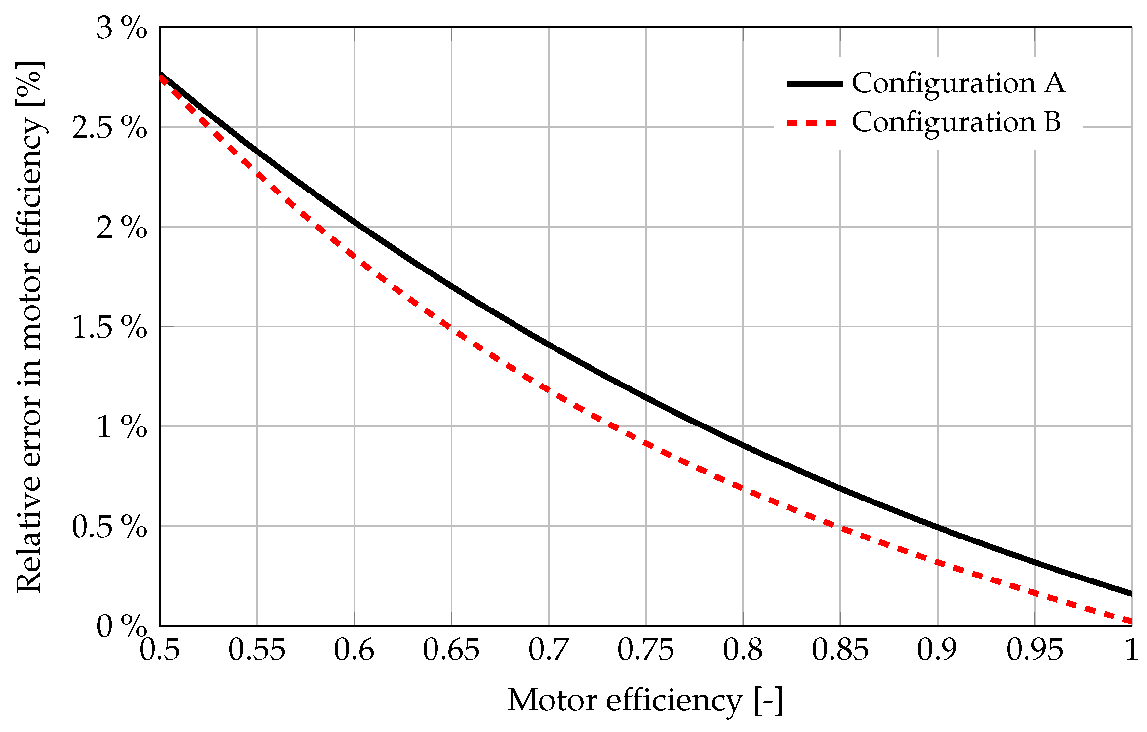
This relative error propagation trend is depicted in Figure 4, showing how the error decreases with higher efficiency values and how the relative error for the efficiency itself converges to zero for ideal machines with $\eta =1$.

The main advantage of this method is that for machines with efficiencies above 80%, the relative error decreases steadily. Additionally, for large machines, measuring mechanical power at the shaft can be difficult and costly due to the need for specialized instruments, making the conventional error method a preferred choice. However, this method has limitations: it does not provide reliable uncertainty for machines with efficiencies below 70%, and for small machines, measuring losses becomes difficult due to low power loss values.

2.4. Configurations A & B Uncertainties

Once the losses are modelled and the sources of uncertainty have been determined, it is possible to determine the measurements relative and absolute errors. In fact, by solving the error propagation equation for a 30 kW electrical motor, the general formulation of the absolute error becomes:

$$\Delta P_{\mathrm{loss}}=\pm {\left[\sum {\left({\displaystyle \frac{\partial P_{\mathrm{loss}}}{\partial P_i}}\right)}^2·\Delta P_i^2\right]}^{0.5}$$

(27)

that can be also computed as:

$$\Delta P_{\mathrm{loss},\mathrm{A}}={\left(\Delta P_{\mathrm{wat},\mathrm{cool},\mathrm{A}}^2+\Delta P_{\mathrm{ins},\mathrm{box}}^2+\Delta P_{fr,\mathrm{conv}/\mathrm{rad},\mathrm{A}}^2+\Delta P_{fr,\mathrm{cond},\mathrm{A}}^2+\Delta P_{\mathrm{leakage}}^2+\Delta P_{\mathrm{air},\mathrm{vent},\mathrm{A}}^2\right)}^{0.5}$$

(28)

or

$$\Delta P_{\mathrm{loss},\mathrm{B}}={\left(\Delta P_{\mathrm{wat},\mathrm{cool},\mathrm{B}}^2+\Delta P_{\mathrm{surf},\mathrm{motor}}^2+\Delta P_{fr,\mathrm{conv}/\mathrm{rad},\mathrm{B}}^2+\Delta P_{fr,\mathrm{cond},\mathrm{B}}^2\right)}^{0.5}$$

(29)

for configurations A and B, respectively. Regardless of the configuration, the relative error can be finally derived as:

$$\mathrm{Relative}\mathrm{error}={\displaystyle \frac{\Delta P_{\mathrm{loss}}}{P_{\mathrm{loss}}}}$$

(30)

3. Measurement Methodology

3.1. Test Bench Setup

An experimental test bench (Figure 5) was built to evaluate a three-phase 30 kW asynchronous motor. Its efficiency as a function of the motor load is reported in

Table 1. Efficiency values of Rowan MEC160L electrical motor.

Load [%]	Efficiency [-]
25	87.8
50	91.5
75	93.0
100	92.2

. The motor is coupled with a centrifugal pump with a rated power of 22 kW which serves as an adjustable load/brake.

A schematic of the experimental setup is shown in Figure 6. In this configuration, two water tanks are used for the storage and discharge of the cooling fluid, respectively. The three-way valve discharges the cooling fluid out of the system until stable conditions are reached, then the discharge tank begins to fill. The discharge flow rate is measured using a load cell installed beneath the discharge basin. As the current setup is confined to low flow rates due to the outlet tank limited volume, for real power plant applications and continuous monitoring, the use of a clamp-on flowmeter installed upstream of the electrical equipment is recommended. A torque sensor and a rotary encoder are positioned on the shaft to have a further measure of the mechanical power. The measuring of temperature relies on the thermo-resistances up- and downstream of the motor. The thermocamera measures motor surface temperatures, although, as proven later, the associated losses can be neglected.

The evaluation of losses and efficiency of the electrical motor requires the measurement of the cooling water inlet and outlet temperature ($T_{wat,in}$ and $T_{wat,out}$), motor external surface and frame temperature ($T_{surf}$, $T_{frame}$), ambient temperature ($T_{out}$), electrical power absorbed ($P_{el}$) and cooling water flow rate ($Q_{water}$). Since the test bench is not equipped with auxiliary ventilation systems, ventilation losses will be neglected from now on ($P_{\mathrm{air},\mathrm{vent}=0}$).

In addition, torque and rotational speed of the motor shaft were also measured to compute the mechanical power ($P_{mech}$), that is exploited as a metric to validate the accuracy of electrical power measurements. Equation (31) shows the relationship between electrical power measurements and mechanical power at the motor shaft:

$$P_{mech}=P_{el}-P_{loss}={\displaystyle \frac{C·w}{1000}}$$

(31)

The uncertainties of each measurement were calculated and incorporated into the overall uncertainty analysis.

3.2. Application to a Real Power Plant

The methodology described in the previous section has a twofold utility in a real HPP. In fact, the described methodology can be applied to instantly compute and evaluate the electrical efficiency of the system. Nevertheless, through a decision tree-based approach that is reported in Figure 7, it is also possible to identify components with minor failures or those operating under anomalous conditions. Regardless of the scope, it is necessary to know the nominal characteristics of some components, as the health component monitoring can be intended as a supplementary operation. If the nameplate characteristics are not available, they can usually be computed according to international standards. In any case, the driving factor is the theoretical specific hydraulic energy, $e_{i,\mathrm{plant}}$, which refers to the amount of energy per unit mass of fluid that can theoretically be extracted or is available in a hydraulic system. Following the Italian CEI 60041 standard [5], $e_{i,\mathrm{plant}}$ is expressed as:

$$e_{i,\mathrm{plant}}={\displaystyle \frac{\rho ·g·Q_i·H}{1000}}$$

(32)

with $Q_i$ as the water discharge rate at the evaluated condition and H as the hydraulic head.

As preliminary operations, the distributor opening and water level are varied, and synchronized measurements are taken to record these settings along with the corresponding electrical power output. The expected electrical power values ($P_{\mathrm{el},\exp }$) are extrapolated from the hydropower plant’s commissioning data to serve as a baseline for comparison. At the same time, the generator’s expected efficiency ${\eta }_{\mathrm{gen},\exp }$ is determined from its characteristic curve to predict its performance under the given conditions. After these steps, the methodology previously described can be finally applied to measure both the current electrical power and the generator efficiency. To discover possible sources of efficiency loss, a series of comparisons can be then carried out (Figure 7).

First, the measured electrical power output ($P_{\mathrm{el}}$) is compared with the expected value ($P_{\mathrm{el},\exp }$). If the two values are equal ($P_{\mathrm{el}}=P_{\mathrm{el},\exp }$), the next step involves verifying the generator’s efficiency. If the measured efficiency (${\eta }_{\mathrm{gen}}$) matches the expected efficiency (${\eta }_{\mathrm{gen},\exp }$), it indicates that the overall plant is functioning as expected. However, if ${\eta }_{\mathrm{gen}}$ does not match ${\eta }_{\mathrm{gen},\exp }$, the inefficiency is attributed to a generator-related issue.

If the measured electrical power output ($P_{\mathrm{el}}$) does not match the expected value ($P_{\mathrm{el},\exp }$), further checks are conducted. If the generator’s efficiency is as expected (${\eta }_{\mathrm{gen}}={\eta }_{\mathrm{gen},\exp }$), the inefficiency is attributed to hydraulic or mechanical problems. If the generator’s efficiency also deviates from the expected value (${\eta }_{\mathrm{gen}}\ne {\eta }_{\mathrm{gen},\exp }$), an additional comparison is made between the lack of electrical power ($P_{\mathrm{el},\mathrm{lack}}$, the difference between expected and measured electrical output) and the extra generator losses ($P_{\mathrm{gen},\mathrm{extra}}$, the difference between measured and expected generator losses). If $P_{\mathrm{el},\mathrm{lack}}$ equals $P_{\mathrm{gen},\mathrm{extra}}$, the inefficiency is attributed solely to a generator-related issue. Otherwise, if $P_{\mathrm{el},\mathrm{lack}}$ does not equal $P_{\mathrm{gen},\mathrm{extra}}$, the inefficiency is attributed to both generator-specific issues and problems in other components.

Finally, if inefficiencies are identified, a warning message is issued to the plant manager, detailing the nature of the problem and necessary corrective actions. Regardless of whether issues are detected and addressed or no discrepancies are found, the monitoring cycle is reiterated to ensure continuous optimization of plant performance.

4. Results and Discussion

The first part of the results focuses on a comparison between the two configurations when applied to the estimation of the losses of the previously described electrical motor. The aim is to quantitatively demonstrate that the simpler Configuration B method can be as applied with negligible variations from Configuration A. In the second part, the motor efficiency is evaluated according to the Configuration B methodology.

4.1. Comparison Between the Two Configurations

Annex A reports a detailed term-by-term comparison of the losses calculated according to configurations A and B. The discussion will be here focused on the aggregated loss values.

Table 2. Losses distribution in a 30 kW electrical motor—configurations A and B.

Losses	Value (A)	Value (B)	Share (A)	Share (B)	Abs. Error (A)	Abs. Error (B)	Rel. Error (A)	Rel. Error (B)	Abs. Err. (${\mathit{P}}_{\mathit{i}}$)/${\mathit{P}}_{\mathbf{tot}}$ (A)	Abs. Err. (${\mathit{P}}_{\mathit{i}}$)/${\mathit{P}}_{\mathbf{tot}}$ (B)
$P_{\mathrm{wat},\mathrm{cool}}$ [kW]	2.232	2.232	93.25%	93.24%	0.058	0.058	2.62%	2.62%	2.44%	2.44%
$P_{\mathrm{ins},\mathrm{box}}$,$P_{\mathrm{surf},\mathrm{motor}}$ [kW]	0.082	0.149	3.42%	6.22%	0.001	0.018	1.72%	12.27%	0.06%	0.76%
$P_{fr,\mathrm{conv}/\mathrm{rad}}$ [kW]	0.012	0.012	0.50%	0.50%	0.003	0.003	23.26%	23.26%	0.12%	0.12%
$P_{\mathrm{leakage}}$ [kW]	0.067	–	2.80%	–	0.033	–	50.00%	–	1.40%	–
$P_{fr,\mathrm{cond}}$ [kW]	0.001	0.001	0.03%	0.03%	0.000	0.000	14.14%	14.14%	0.00%	0.00%
$P_{\mathrm{loss}}$ [kW]	2.394	2.394	100%	100%	0.059	0.061	2.45%	2.56%	–	–

presents the estimated power losses for each type, their associated uncertainties, and relative errors for both configurations A and B, based on the described theoretical models. The total power loss, uncertainty, and relative error are calculated using Equations (28) and (30) for Configuration A and Equations (29) and (30) for Configuration B. Additionally, the last column of the table shows the ratio of the absolute error of each loss contribution to the total losses for both configurations.

Notably, while the uncertainty in Configuration B is slightly higher than in Configuration A, this configuration is non-invasive, as it does not require modifying the plant. Both configurations exhibit similar loss values with comparable absolute uncertainties. Consequently, Configuration B can be adopted as it offers similar error levels while eliminating the need for changes to the electrical machine and plant.

As shown in Figure 8, the dominant source of losses is the water cooling system, which accounts for 93.25% of losses in both Configuration A and B. The heat transmitted through the insulation box in Configuration A (3.42%) and the heat lost by the motor surface in Configuration B (6.22%) both also have non-negligible contributions. It is worth noting that, although there appears to be a large difference in these losses between the two methods, Configuration B also takes leakage losses into account, whereas these are treated separately in the first method; thus,

$$P_{\mathrm{ins},\mathrm{box},\mathrm{A}}+P_{\mathrm{leakage},\mathrm{A}}=P_{\mathrm{surf},\mathrm{motor},\mathrm{B}}$$

(33)

The remaining losses, attributed to the heat exchange from the shaft and motor frame have a marginal influence, with the conduction term that is almost negligible (<0.03%).

The sensitivity analysis indicates that the relative error in the mathematical model decreases as the motor’s efficiency increases for both configurations, as shown in Figure 9. For a nominal power of 30 kW and total losses, the motor achieves an efficiency of 92%, that reflects in a relative error of $\pm 0.229\%$ and $\pm 0.024\%$ for Configuration A and B, respectively.

4.2. Efficiency Computation

The previous section highlights that Configuration B is more than capable of estimating motor efficiency, even if it based on a simplified measuring method. In addition, Configuration B exhibits a minor error as the motor efficiency increases. Configuration B was further utilized to test the motor under three different load values: 14 kW, 19 kW, and 25 kW, corresponding to 47%, 63%, and 83% of the nominal load, respectively.

During the tests, the measurement quantities described previously were collected simultaneously under steady-state conditions. Consequently, after the motor start-up, the variation in water temperatures in the cooling circuit and in the thermocouples positioned on the motor’s external surface was monitored. Preliminary investigations showed that the cooling fluid temperature exhibits the longest transition time to reach steady-state conditions among the observed quantities. Only after the stabilization of these temperatures could the system be assumed to be in steady-state conditions, allowing the acquisition of all relevant quantities to begin. Steady-state operation of the motor was considered achieved when a defined threshold temperature value was reached, determined as:

$${\displaystyle \frac{\left|\Delta T_{i+1}-\Delta T_i\right|}{\Delta T_i}}\le 0.01$$

(34)

where $\Delta T_i=T_{\mathrm{wat},\mathrm{out},i}-T_{\mathrm{wat},\mathrm{in},i}$ is the temperature difference between inlet and outlet of the cooling system at the i-th time. Data were collected over a interval of 10 min, and the measurements obtained by the different sensors were then elaborated and synchronized. The efficiency of the motor, based on the heat loss-based and “standard” power methods can be then calculated using the following expressions:

$${\eta }_{\mathrm{calorimetric}}={\displaystyle \frac{P_{\mathrm{el}}-P_{\mathrm{loss}}}{P_{\mathrm{el}}}}$$

(35)

$${\eta }_{\mathrm{power}}={\displaystyle \frac{P_{\mathrm{mech}}}{P_{\mathrm{el}}}}$$

(36)

Table 3. Electrical, mechanical power, and losses at different motor loads—Configuration B.

Quantity	14 kW	19 kW	25 kW
$P_{\mathrm{el}}$ [ $\mathrm{k}$$\mathrm{W}$]	14 ± 0.3	19.2 ± 0.4	24.8 ± 0.5
C [ $\mathrm{N}$$\mathrm{m}$]	41.1 ± 0.1	57.1 ± 0.1	41.1 ± 0.1
w [rpm]	2984.2 ± 0.85	2975.2 ± 0.8	2964 ± 0.6
$P_{\mathrm{mech}}$ [ $\mathrm{k}$$\mathrm{W}$]	12.84 ± 0.03	17.79 ± 0.03	23.04 ± 0.03
$P_{\mathrm{wat},\mathrm{cool}}$ [ $\mathrm{k}$$\mathrm{W}$]	1.1 ± 0.1	1.4 ± 0.1	1.8 ± 0.1
$P_{\mathrm{surf},\mathrm{motor}}$ [ $\mathrm{k}$$\mathrm{W}$]	0.009 ± 0.002	0.001 ± 0.004	0.001 ± 0.0004
$P_{fr,\mathrm{conv}/\mathrm{rad}}$ [ $\mathrm{k}$$\mathrm{W}$]	0.003 ± 0.001	0.003 ± 0.001	0.005 ± 0.001
$P_{fr,\mathrm{cond}}$ [ $\mathrm{k}$$\mathrm{W}$]	0.014 ± 0.002	0.015 ± 0.002	0.017 ± 0.002
$P_{\mathrm{loss}}$ [ $\mathrm{k}$$\mathrm{W}$]	1.2 ± 0.1	1.4 ± 0.1	1.8 ± 0.1
${\eta }_{\mathrm{calorimetric}}$ [-]	0.9175 ± 0.0083	0.9281 ± 0.0065	0.9265 ± 0.0055
${\eta }_{\mathrm{power}}$ [-]	0.9184 ± 0.0184	0.9275 ± 0.0186	0.9274 ± 0.0185

presents the measurements of the three tests, further detailed in Figure 10. The results show that the relative error associated with heat loss-based method losses decreases as the motor load increases. This aspect is particularly relevant since power losses increase with motor load. Therefore, a marginal error in measurements can be expected when applied to electrical units operating in regular duty scenarios. The estimated efficiency ${\eta }_{\mathrm{calorimetric}}$ is perfectly in agreement with the efficiency calculated using the standard method ${\eta }_{\mathrm{power}}$, evaluated according to Equation (23).

A detailed comparison between the two methods is presented in Figure 11, which visualizes the relative error propagation as a function of motor efficiency for the different approaches. The trend observed for Configuration B suggests that the proposed method exhibits high relative errors when motor efficiency is low, with a notable relative error ranging between 13% and 16%. This finding highlights a limitation of applying this methodology to low-grade motors, where the traditional approach should be preferred, since its relative error $\approx 2\%$. However, in HPPs characterized by high-grade electrical units ($\eta >80\%$), the heat loss-based method becomes the favorable choice, as the relative error becomes negligible as efficiency approaches unity. This trend can be observed at all operating conditions of the considered motor.

5. Conclusions

The manuscript introduces a novel methodology for the online continuous monitoring of hydropower plant efficiency, called the heat loss-based method. This method enables the measurement of both electrical generator losses and electrical input power, along with their associated uncertainties. Compared to traditional monitoring systems, it is non-invasive and can be applied without significant modifications, regardless of turbine size or plant layout.

Two different approaches to the heat loss-based method have been introduced, namely Configuration A and Configuration B, which differ in their treatment of hot surfaces. Compared to Configuration A, Configuration B is simpler to implement in real-world scenarios, as it does not require building an insulation box to enclose the electric units. Both configurations achieve a Type-B relative error below the 1% threshold of the traditional method when motor efficiency exceeds 80%. Furthermore, the manuscript also demonstrates how the heat loss-based method can serve as a low-level health monitoring system, providing insights into failing components.

The proposed method exhibits great advantages also considering possible sensor calibration errors, environmental effects, and integration challenges have been considered. However, the proposed method is primarily based on the temperature difference between the inlet and outlet water of the cooling system, and since fluid cooling represents the major source of thermal losses, the influence of absolute sensor calibration errors is significantly reduced. The methodology relies on differential measurements, making it less sensitive to minor calibration offsets. Therefore, calibration errors are expected to have a minimal impact on the accuracy of the results.

Similarly, the effect of environmental conditions is also considered negligible, as these primarily influence secondary losses such as radiation and convection from exposed surfaces, which constitute a minor portion of the total energy balance. As a result, the proposed method remains robust under varying ambient conditions. Regarding integration challenges, the use of clamp-on fluxmeters and the availability of data from the HPP control system significantly simplify the installation process, eliminating the need for plant shutdowns.

The proposed heat loss-based method has been tested using an experimental test rig equipped with a 30 kW electric motor. A comparison between the two configurations shows that, while Configuration A exhibits slightly lower relative error, Configuration B is preferable due to its easier installation and fewer required measurements. Finally, a comparison of Configuration B measurements with the traditional method at different motor loads demonstrates that the heat loss-based method achieves the same electrical efficiency estimations while maintaining a lower relative error across all operating conditions. Although the heat loss-based method exhibits higher errors at low motor efficiency (${\eta }_{\mathrm{el}}<0.8$), it outperforms the standard method for motor grades typical of hydropower plants.