AI-Powered Convolutional Neural Network Surrogate Modeling for High-Speed Finite Element Analysis in the NPPs Fuel Performance Framework

Abstract

Convolutional Neural Networks (CNNs) are proposed for use in the nuclear power plant domain as surrogate models to enhance the computational efficiency of finite element analyses in simulating nuclear fuel behavior under varying conditions. The dataset comprises 3D fuel pellet FE models and involves 13 input features, such as pressure, Young’s modulus, and temperature. CNNs predict outcomes like displacement, von Mises stress, and creep strain from these inputs, significantly reducing the simulation time from several seconds per analysis to approximately one second. The data are normalized using local and global min–max scaling to maintain consistency across inputs and outputs, facilitating accurate model learning. The CNN architecture includes multiple dense, reshaping, and transpose convolution layers, optimized through a brute-force hyperparameter tuning process and validated using a 5-fold cross-validation approach. The study employs the Adam optimizer, with a significant reduction in computational time highlighted using a GPU, which outperforms traditional CPUs significantly in training speed. The findings suggest that integrating CNN models into nuclear fuel analysis can drastically reduce computational times while maintaining accuracy, making them valuable for real-time monitoring and decision-making within nuclear power plant operations.

1. Introduction

In nuclear engineering field, computational modeling software is used to assess the behavior of systems, structures, and components (SCCs) governed by partial differential equations (PDEs) [1]. Usually, such tools solve the PDE directly with the use of finite element analysis (FEA). FEA breaks SSCs into a finite number of discrete elements and nodes, allowing FEA software to solve the equations efficiently. FEA-based simulations rely on iteratively solving PDEs that correspond to specific physics models. Typically, the analysis of the problem to be investigated needs to be discretized into several timesteps. Increasing the number of timesteps results in a solution with higher resolution in the time domain, but it typically leads to a higher computational cost. FEA uses predictions of the previous step to solve the current status at each iteration. The order of PDEs and the density of the mesh increase can lead to computationally expensive simulations. Reduced-order modeling (ROM) and surrogate models are considered useful methods for this purpose. In order to reduce the dimensionality of high-order models, the ROM approach is the most commonly deployed, while surrogate models are used to substitute FEA.

Traditional ROM, including principal component analysis and proper orthogonal decomposition, are limited by their intrinsic linearity. Consequently, solutions involving artificial intelligence, such as Artificial Neural Networks (ANNs), Convolutional Neural Networks (CNNs) [2], and Multilayer Perceptrons (MLPs), have proven to be alternative solutions for reducing the dimensionality of non-linear systems in physics [3,4,5]. The rapid development of surrogate models in the AI field can be detected by their capacity to evaluate both linear and non-linear functions that are inherent in their weights.

In the nuclear reactor fuel engineering domain, surrogate models can represent an opportunity to enhance the computational efficiency of simulations, especially when dealing with phenomena like pellet-cladding interaction (PCI) and pellet-cladding mechanical interaction (PCMI). These interactions are mechanistically complex, coupling fuel’s neutronic and thermal behaviors, which are challenging to model with high fidelity, due to the computationally expensive nature of detailed simulations characterized by multiphysics and multiscale domains. There are few studies in the open literature related to surrogate modeling in the nuclear field, especially for fuel performance assessment.

This study [6] proposes a Long Short-Term Memory Stacked Ensemble (LSTM-SE) surrogate model for predicting the microstructural evolution and mechanical properties of AISI 316L stainless steel fuel cladding under different temperature and radiation dose rates. Precipitation kinetics were modeled with a kinetic Monte Carlo (KMC) approach, and finite element method (FEM) analysis was performed for evaluating the mechanical properties. The surrogate model proved very accurate (error range of ≤6%) and was 1000× faster compared with conventional physics-based simulations.

A surrogate model with ANNs with the purpose of improving the safety of nuclear plants via a systematic study of the response of containment structures under internal pressure was developed in [7]. A finite element model, validated with experimental data, was used for performing a Sobol sensitivity study with regard to material uncertainty. The study demonstrated the significant role of concrete compressive capacity and the force of prestress, with varying importance for different levels of pressure. The surrogate model, replacing expensive FE simulations, enabled a wider and more effective investigation of uncertainties. An alternative technique in the nuclear domain employed the Improved Lump Mass Stick (I-LMS) model for the AP1000 nuclear power plant (NPP), thus providing improved accuracy when compared against classical Lump Mass Stick (LMS) models [8]. Through applying the Kriging surrogate model, mass condensation optimization for shear walls was achieved successfully. The I-LMS model reduced the error by frequency from 23.04% to 6.57%, increased the modal assurance criterion (MAC) value, and showed greater accuracy for structural dynamic response when compared against the finite element model (FEM) analysis.

The present study [9] introduces a hybrid surrogate model-based multi-objective optimization method for designing spherical fuel element (SFE) canisters in high-temperature gas-cooled reactors (HTGRs). A FE method–discrete element method (FEM–DEM) coupled model was developed for drop analysis, identifying key design variables and constraints. A hybrid radial basis function–response surface method (RBF–RSM) surrogate model was employed to approximate the numerical model, and NSGA-II was used for optimization, demonstrating high accuracy and lower computational expense. Surrogate models to update the Bayesian finite element (FE) model in structural health monitoring (SHM) and damage prognosis (DP) are developed in [10]. A miter gate structural system is analyzed, considering three predominant damage modes. Polynomial chaos expansion (PCE) and Gaussian process regression (GPR) surrogate models are developed and compared with direct FE evaluations. The results show that surrogate-based Bayesian updating achieves sufficient accuracy, while reducing the computational time by approximately 4-fold, demonstrating the feasibility of surrogate models for efficient large-scale structural assessments.

The authors of manuscript [11] successfully applied surrogate-based approaches to core depletion problems, integrating physics-based models like VERA-CS for improved predictive capability. The algorithm provides ROM, which is then utilized for Bayesian estimation for calibrating the neutronic and thermohydraulic parameters. Based on experimental and operational data, the results demonstrated that ROM could help to decrease uncertainty in key reactor attributes.

Therefore, surrogate models offer a time-efficient alternative for simulating complex physical phenomena such as PCMI [12], providing quicker results compared to detailed 2D and 3D fuel code software. Both PCI and PCMI still remain key challenges in the nuclear domain. These phenomena, first observed in water-cooled reactors in the 1960s, have been studied extensively to understand and evaluate their effects on Zircaloy cladding [13]. Fission gas release, involving low-solubility gases, such as Xenon and Krypton, produced during fission, also plays a key role in fuel design. If these gases remain in the fuel pellet, they promote swelling that intensifies mechanical interaction with the cladding. On the other hand, if released into the gas gap, their relatively low thermal conductivity can increase the fuel temperature and possibly lead to cladding cracking. These phenomena are inherently complex and difficult to model, due to their coupling with both neutronic and thermal behavior. Consequently, fuel performance codes depend significantly on the accuracy of their PCMI modeling [14].

Therefore, surrogate models approximate the outcomes of computationally expensive simulations, significantly reducing the required computational time and resources. By employing surrogate models, it is possible to achieve a balance between accuracy and efficiency; they are particularly useful in scenarios where full-scale simulations are excessively expensive. To this end, a surrogate model based on CNNs is proposed to investigate the thermomechanical behavior of a PWR fuel pellet. The results show impressive cost-saving in terms of computational time compared to FE analysis. The surrogate model, once trained, predicts the stress field in less than 1 s, which is much faster compared to full FE analysis, which needs about 17 s (wall time).

2. Materials and Methods

2.1. Data Preparation

The dataset used in this study consists of 13 input features, including pressure, Young’s modulus, Poisson’s ratio, mass density, yield strength, thermal expansion coefficient, and temperature. These features represent material properties and boundary conditions affecting thermomechanical behaviors. Details of the input parameters are collated in

Table 1. Input parameters of FE model for data generation.

	Value	Unit
Mass density	1.036 × 104	[kg/m3]
2. Young’s modulus	1.7 × 1011	[Pa]
3. Poisson’s ratio	3.16 × 10−1	[-]
4. Thermal expansion coefficient	1.027 × 10−5	[K−1]
5. Yield strength	1.5 × 108	[Pa]
6. Specific heat	3.0 × 10−1	[J/kg °C]
7. Thermal conductivity	Fink-Lucuta Model [15]
8. Shear modulus	7.6 × 1010	[Pa]
9. Back stress for implicit creep	0.0	[Pa]
10. Yield stress for implicit creep	1.5 × 108	[Pa]
11. Specific heat	4.8 × 101	[J/(kg·°C)]
12. Centerline temperature	1.2 × 103	[°C]
13. Pressure	2.0 × 106	[Pa]

. In this study, a 3D fuel pellet is implemented in the FE code. In Figure 1, its overall dimensions and 3D finite element (FE) model are presented.

The FE analysis simulates an increase in the rod’s internal pressure due to the fission gas. The boundary conditions of the FE model are defined by a centerline temperature of 1200 °C and a nominal pressure of 2 MPa, corresponding to typical pressurized water reactor conditions. These values vary as the transient progresses. The dataset is generated based on a representative scenario of a standard reactor operation with increasing fuel burnup. The traditional approach involves expensive computational time for integrity assessment, and so a real-time approach cannot be applied. In this case, once the CNN model is trained, the results in terms of displacement, von Mises stress, and creep strain are obtained in ≈1 s. The training dataset comprises 3360 images, considering top, bottom, lateral views of von Mises stress, creep strain, and displacement. The images were generated by the FE code MSC Marc^® (https://hexagon.com/products/marc, accessed on 3 April 2025; MSC Software Corporation, Newport Beach, CA, USA).

The input data were normalized using min–max scaling to ensure compatibility across varying scales. The output data, which included 512 × 512 matrices of creep strain, displacement, and von Mises stress, were also normalized. Outputs were scaled between 0 and 1, based on their global minimum and maximum values, to facilitate model learning [16].

$${\mathrm{x}}_{\mathrm{s}\mathrm{c}\mathrm{a}\mathrm{l}\mathrm{e}\mathrm{d}}={\displaystyle \frac{\mathrm{x}-{\widehat{\mathrm{x}}}_{\mathrm{m}\mathrm{i}\mathrm{n}}}{{\widehat{\mathrm{x}}}_{\mathrm{m}\mathrm{a}\mathrm{x}}-{\widehat{\mathrm{x}}}_{\mathrm{m}\mathrm{i}\mathrm{n}}}},$$

(1)

However, since each image had its own minimum and maximum values which shared identical color values, the scaling was adjusted based on the local minimum and maximum values:

$${\widehat{\mathrm{x}}}_{\mathrm{m}\mathrm{a}\mathrm{x}}={\displaystyle \frac{{\mathrm{x}}_{\mathrm{l}\mathrm{o}\mathrm{c}\mathrm{a}\mathrm{l}\_\mathrm{m}\mathrm{a}\mathrm{x}}-{\mathrm{x}}_{\mathrm{g}\mathrm{l}\mathrm{o}\mathrm{b}\mathrm{a}\mathrm{l}\_\mathrm{m}\mathrm{i}\mathrm{n}}}{{\mathrm{x}}_{\mathrm{g}\mathrm{l}\mathrm{o}\mathrm{b}\mathrm{a}\mathrm{l}\_\mathrm{m}\mathrm{a}\mathrm{x}}-{\mathrm{x}}_{\mathrm{g}\mathrm{l}\mathrm{o}\mathrm{b}\mathrm{a}\mathrm{l}\_\mathrm{m}\mathrm{i}\mathrm{n}}}}$$

(2)

$${\widehat{\mathrm{x}}}_{\mathrm{m}\mathrm{i}\mathrm{n}}={\displaystyle \frac{{\mathrm{x}}_{\mathrm{l}\mathrm{o}\mathrm{c}\mathrm{a}\mathrm{l}\_\mathrm{m}\mathrm{i}\mathrm{n}}-{\mathrm{x}}_{\mathrm{g}\mathrm{l}\mathrm{o}\mathrm{b}\mathrm{a}\mathrm{l}\_\mathrm{m}\mathrm{i}\mathrm{n}}}{{\mathrm{x}}_{\mathrm{g}\mathrm{l}\mathrm{o}\mathrm{b}\mathrm{a}\mathrm{l}\_\mathrm{m}\mathrm{a}\mathrm{x}}-{\mathrm{x}}_{\mathrm{g}\mathrm{l}\mathrm{o}\mathrm{b}\mathrm{a}\mathrm{l}\_\mathrm{m}\mathrm{i}\mathrm{n}}}}$$

(3)

The following approach was used to ensure uniform color mapping: Since each image could have different intensity ranges but the same colormap, normalizing within a global range was used to prevent misleading interpretations. Furthermore, the dataset was divided into training, validation, and test sets. A 5-fold cross-validation approach [17] was used for model evaluation. In this process, the training dataset was split into five subsets, with four subsets used for training and one for validation.

This ensured that the model was validated on different portions of the dataset during training, reducing overfitting and increasing robustness. For better insight into the problem, examples of expected CNN outputs are presented in Figure 2 and Figure 3, showing the mesh from the top (Figure 2) and from the left-side view (Figure 3).

2.2. Convolutional Neural Network (CNN) Architecture

The core model employed in this study is a Convolutional Neural Network (CNN) (or rather, one of its variations [18,19]), designed to predict spatially distributed outputs (creep strain, displacement, and von Mises stress). The mathematical operations behind each layer of the CNN are described in Section 2.2.1, Section 2.2.2, Section 2.2.3, Section 2.2.4, Section 2.2.5, Section 2.2.6, Section 2.3 and Section 2.4.

2.2.1. Input Layer

The input vector x ϵ R represents the material properties and environmental parameters, denoted as follows:

$$\mathrm{x}=\left[{\mathrm{x}}_1,{\mathrm{x}}_2,\dots ,{\mathrm{x}}_{13}\right]$$

(4)

where $x_i$ corresponds to specific input features, such as pressure, Young’s modulus, and temperature.

2.2.2. Dense Layers

Three dense (fully connected) layers are used to extract high-level features from the input data. Each layer applies a linear transformation followed by a non-linear activation function [19,20]:

$${\mathrm{z}}^{\left(\mathrm{l}\right)}=\mathsf{\sigma }\left({\mathrm{w}}^{\left(\mathrm{l}\right)}{\mathrm{z}}^{\left(\mathrm{l}-1\right)}+{\mathrm{b}}^{\left(\mathrm{l}\right)}\right)$$

(5)

where

• $z^{\left(l-1\right)}$ is the output of the previous layer (or input for $l=1$);
• $w^{\left(l\right)}$ and $b^{\left(l\right)}$ are the weight matrix and bias vector of layer $l$;
• $\sigma$ is the ReLU activation function [21]:

$$\mathsf{\sigma }\left(\mathrm{x}\right)=\mathrm{m}\mathrm{a}\mathrm{x}\left(0,\mathrm{x}\right)$$

(6)

The number of neurons in the dense layers is determined through hyperparameter optimization, with values ranging from 128 to 512. Assuming that N is the number of neurons in the first dense layer, the number of neurons in the second and third layers will be equal to 4 N and 8 N, respectively.

2.2.3. Reshaping Layer

The output of the dense layers is reshaped into a 2D matrix as follows [22]:

$${\mathrm{Z}}_{\mathrm{r}\mathrm{e}\mathrm{s}\mathrm{h}\mathrm{a}\mathrm{p}\mathrm{e}\mathrm{d}}={\mathbb{R}}^{64\times 64\times 1}$$

(7)

2.2.4. Resize Layer

The resize layer [23] is used to adjust the dimensions of the feature map (the output of the previous layer). Mathematically, this operation involves interpolation or downscaling/upscaling. Assuming the input tensor has dimensions H_in × W_in × C_in, resizing transforms it to a new shape, H_out × W_out × C_out, while keeping C_in = C_out = 1 (the number of channels, which is equal to 1 for grayscale images). While the currently proposed model is designed for 2D images, the model was created with the idea that, in the future, it might be converted into a 3D matrix generator. However, 2D implementation is used here, due to the large cost of 3D modeling in terms of the dataset and computing power.

Bilinear interpolation is used (common in resizing) for each pixel value p(x,y) in the resized output:

$$\mathrm{p}(\mathrm{x},\mathrm{y})=\sum _{\mathrm{i}=0}^1\sum _{\mathrm{j}=0}^1{\mathrm{w}}_{\mathrm{i}\mathrm{j}}\mathrm{p}\left({\mathrm{x}}_{\mathrm{i}},{\mathrm{y}}_{\mathrm{j}}\right)$$

(8)

where

• p(x_i,y_j) are the nearest input pixels;
• w_ij are the bilinear interpolation weights, calculated based on the distance of the output pixel to the input pixel grid.

Putting theory aside, we resized the reshaped input, which had a 64 × 64 × 1 shape, into an image with a 256 × 256 × 1 shape. In other words, the resolution was increased by 4 times (upscaling).

2.2.5. Transpose Convolution Layer

To increase the spatial resolution, a transpose convolution layer [23,24] is applied. The mathematical operation is defined as follows:

$$\mathrm{O}(\mathrm{x},\mathrm{y},{\mathrm{c}}_{\mathrm{o}\mathrm{u}\mathrm{t}})=\sum _{\mathrm{i}=0}^{\mathrm{k}-1}\sum _{\mathrm{j}=0}^{\mathrm{k}-1}\sum _{{\mathrm{c}}_{\mathrm{i}\mathrm{n}}}\mathrm{K}\left(\mathrm{i},\mathrm{j},{\mathrm{c}}_{\mathrm{i}\mathrm{n}},{\mathrm{c}}_{\mathrm{o}\mathrm{u}\mathrm{t}}\right)\mathrm{I}\left(\mathrm{x}-\mathrm{i},\mathrm{y}-\mathrm{j},{\mathrm{c}}_{\mathrm{i}\mathrm{n}}\right),$$

(9)

Here,

• O (x,y,c_out) is the output feature map at position (x,y);
• K (i,j,c_in,c_out) is the convolution kernel;
• I (x_i,y_j,c_in) is the input feature map.

With kernel size, stride, and padding, this layer doubles the spatial dimensions while applying convolution kernels. The stride determines how much the output feature map is “stretched” by inserting zeros between pixels in the input feature map. When stride > 1, zeros are interleaved between pixels in the input before the kernel is applied, effectively increasing the spatial resolution. In our work, we used stride = 2, which doubled the spatial resolution. In addition, a 3 × 3 kernel size was used for relatively sharp pixel values, and a number of filters of 3 × N_filters was selected. In this case, N_filters was the parameter optimized using hyperparameter optimization.

2.2.6. Output Layer

A final convolution layer with a kernel produces the predicted output matrix, which is an image with a 512 × 512 × 1 shape. A visualization of the entire architecture is provided in Figure 4, showing how the inputs are converted into grayscale images.

2.3. Optimization and Validation

The Adam optimizer was used with a learning rate of 0.01, and training was conducted over 100 epochs. The model’s hyperparameters, including the number of dense-layer neurons and filters in the transpose convolution layer, were optimized using a brute-force search. A 5-fold cross-validation approach was employed to ensure robust evaluation, with the average validation loss across folds used to select the best-performing model. The final evaluation was conducted on a reserved test set (10% of the data).

$${\mathrm{L}\mathrm{o}\mathrm{s}\mathrm{s}}_{\mathrm{a}\mathrm{v}\mathrm{e}\mathrm{r}\mathrm{a}\mathrm{g}\mathrm{e}\mathrm{d}}={\displaystyle \frac{1}{\mathrm{K}}}\sum _{\mathrm{k}=1}^{\mathrm{K}}{\mathrm{L}\mathrm{o}\mathrm{s}\mathrm{s}}_{\mathrm{k}}$$

(10)

where K is the number of folds and Loss_k is the loss value of a single fold. In our work, this value was computed using the Mean Squared Error:

$${\mathrm{L}\mathrm{o}\mathrm{s}\mathrm{s}}_{\mathrm{k}}={\displaystyle \frac{1}{\mathrm{M}}}\sum _{\mathrm{i}=1}^{\mathrm{M}}{\left({\mathrm{y}}_{\mathrm{i}}-{\widehat{\mathrm{y}}}_{\mathrm{i}}\right)}^2$$

(11)

where M is the number of samples in the dataset, y_i is the real value of sample i, and ${\widehat{y}}_i$ is the estimated value for the same sample.

2.4. Information About Tools and Equipment

The CNN was developed on a workstation based on Intel(R) Core(TM) i9-9820X CPU @ 3.30 GHz, 10 core, 20 logical processor (Intel Corporation, Santa Clara, CA, USA). For model training, Python 3.10 [25] was used, and the network was developed using Tensorflow 2.13.0 [26] on the Anaconda [27] framework. The developed model was saved in h5 file format, which allows for fast loading and compact storage, and ensures that no data are lost.

3. Results

3.1. Quantitative Evaluation: Mean Squared Error (MSE)

To quantify the model’s performance, the Mean Squared Error (MSE) [28] between the real and predicted output matrices was calculated. The MSE was computed for each prediction type (displacement, von Mises stress, creep strain), providing an overall measure of the model’s accuracy.

The average MSE for each prediction type is shown in

Table 2. MSEs for displacement (top variant) model with different sets of neurons. Results obtained from 5-fold validation.

	N	128	256	384	512
Nfilters
192		0.001544422	0.001832612	0.002114617	0.002725448
384		0.002859113	0.0022291	0.002043019	0.002062435
576		0.001929024	0.002103111	0.008665383	0.00210098
768		0.002305543	0.002289356	0.002366306	0.001929906

,

Table 3. MSEs for displacement (left variant) model with different sets of neurons. Results obtained from 5-fold validation.

	N	128	256	384	512
Nfilters
192		0.001203205	0.001335009	0.001183916	0.001158133
384		0.001567844	0.001129127	0.001284317	0.001230932
576		0.00131301	0.001146487	0.002820604	0.017106705
768		0.001187524	0.001512092	0.00349265	0.001189423

,

Table 4. MSEs for von Mises (top variant) model with different sets of neurons. Results obtained from 5-fold validation.

	N	128	256	384	512
Nfilters
192		0.000678745	0.000876072	0.000950538	0.001664605
384		0.000862308	0.001562658	0.001013303	0.001174877
576		0.000749681	0.001686655	0.001621389	0.000712151
768		0.000681306	0.000769311	0.0009108	0.000787454

,

Table 5. MSEs for von Mises (left variant) model with different sets of neurons. Results obtained from 5-fold validation.

	N	128	256	384	512
Nfilters
192		0.000691089	0.000746355	0.000983278	0.000899574
384		0.000719873	0.000703136	0.000792825	0.000775237
576		0.001265486	0.000841125	0.004567229	0.019497849
768		0.003099162	0.009136992	0.03097271	0.001161165

,

Table 6. MSEs for creep strain (top variant) model with different sets of neurons. Results obtained from 5-fold validation.

	N	128	256	384	512
Nfilters
192		0.002292389	0.001308951	0.001273264	0.001866534
384		0.124179673	0.001265201	0.001848137	0.014220319
576		0.003963655	0.002191666	0.00145515	0.100486011
768		0.001248196	0.001434278	0.002076672	0.00181988

and

Table 7. MSEs for creep strain (left variant) model with different sets of neurons. Results obtained from 5-fold validation.

	N	128	256	384	512
Nfilters
192		0.000599372	0.000634892	0.000670759	0.000770739
384		0.000693904	0.001149922	0.000659028	0.000774915
576		0.000646266	0.000639543	0.001948988	0.000833224
768		0.000706057	0.000689143	0.000709572	0.000797344

. These tables show the results obtained via 5-fold validation for a selection of neurons and filters. In the tables, N is the number of neurons and N_filters is the number of filters. The green shading highlights the best-performing configurations, while the red shading indicates the worst-performing one.

The best setups were used as the final models.

As shown in Table 2, Table 4 and Table 6, models with fewer neurons outperformed those with a higher number of neurons in the present study. While it is possible that more complex models could eventually surpass the simpler ones with extended training time, this approach is not currently feasible, due to computational constraints and time limitations.

Moreover, the ability of lighter models to predict quickly and accurately is highly advantageous, especially in real-time applications, where speed and efficiency are critical. These models provide a practical balance between performance and resource utilization, making them suitable for deployment in various scenarios.

On the other hand, Table 3, Table 5 and Table 7 highlight the importance of finding the right balance between the number of neurons and filters. This balance is crucial for optimizing model performance, as it ensures that the model is neither too simple to capture the necessary patterns, nor too complex to train efficiently within reasonable timeframes.

A larger dataset can improve CNN performance. However, it must be pointed out that additional data could significantly alter the best-performing setups. Depending on whether the new data are simpler or more complex, the optimal configurations of neurons and filters might change accordingly.

3.2. Comparison of Real and Predicted Outputs

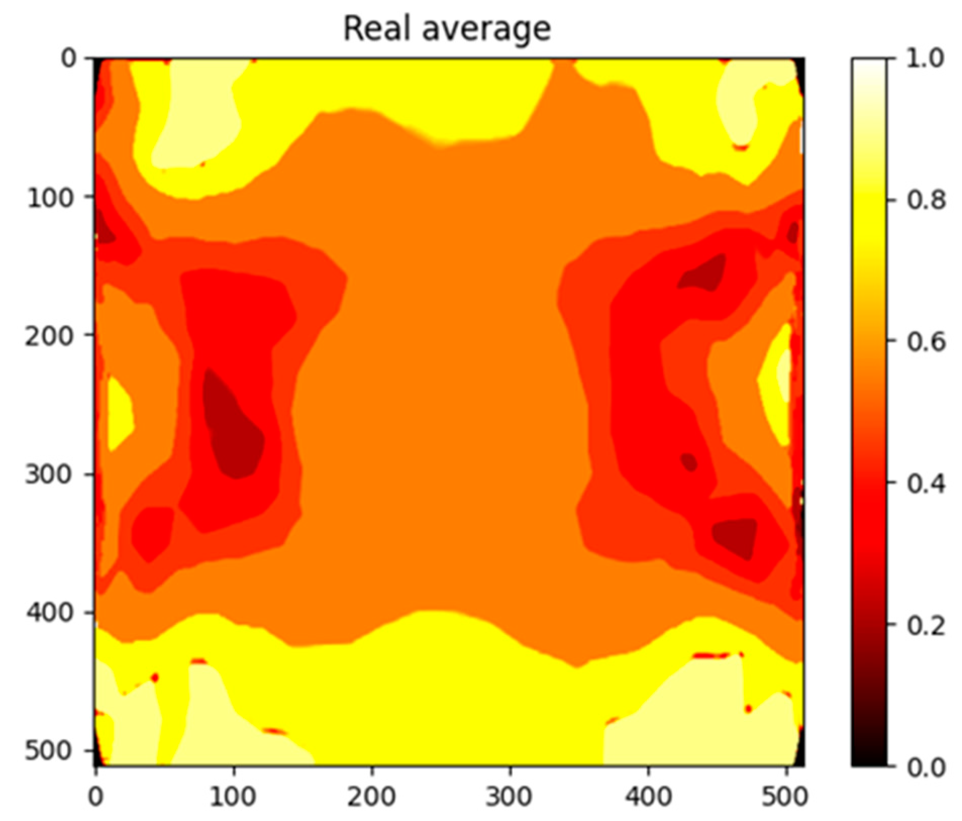
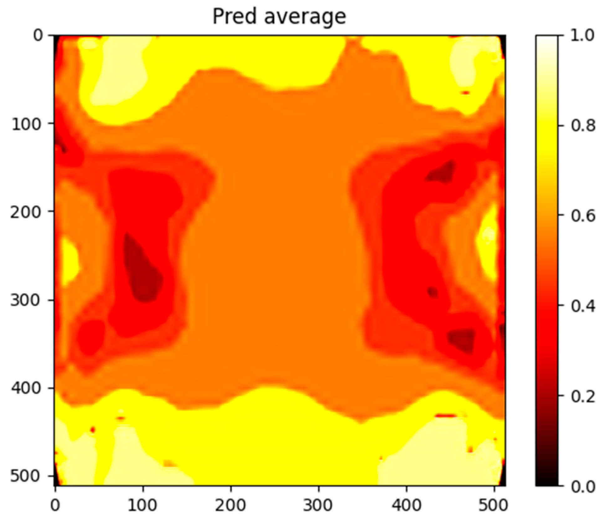
The model’s performance was first evaluated by comparing the predicted output matrices (creep strain, displacement, and von Mises stress) with the actual ground truth data. Visual comparisons of the real and predicted images were made for several test samples, highlighting the model’s ability to accurately predict spatial variations in mechanical properties.

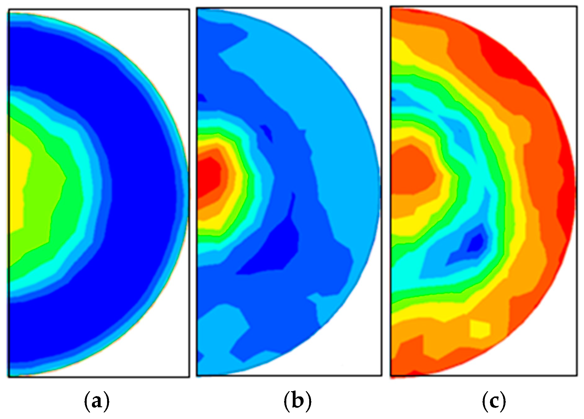
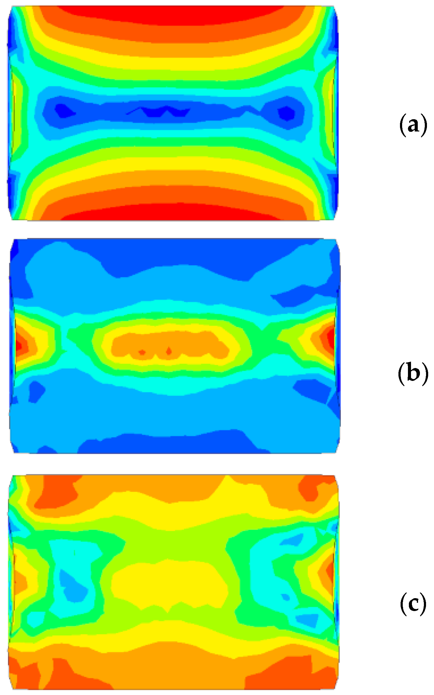
Figure 5 and Figure 6 show the real and predicted images for a sample from the test set. The predicted images closely resemble the actual patterns, demonstrating the model’s ability to capture the complex spatial relationships between input features and the target outputs.

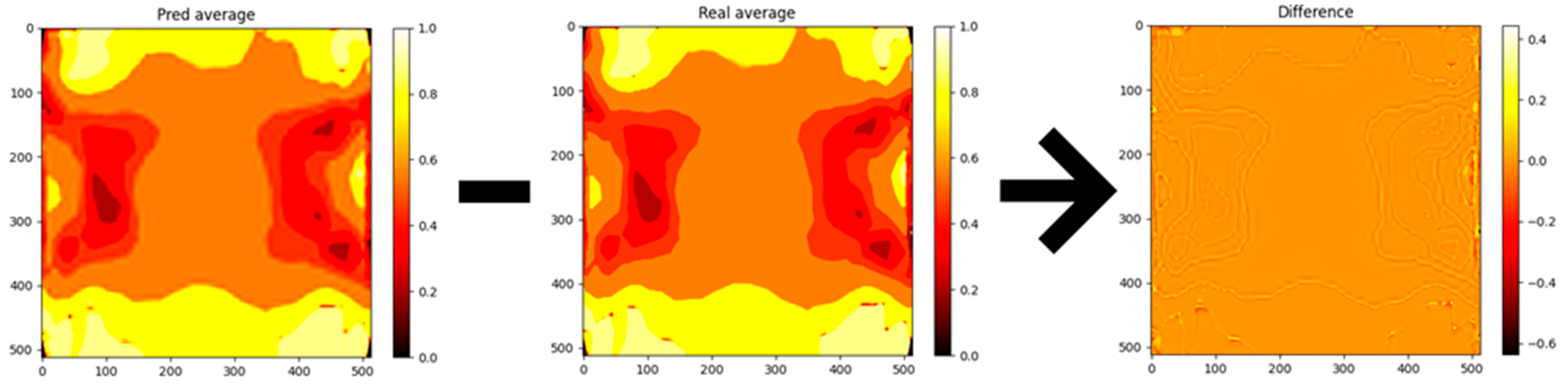
3.3. Visualizing Error Distributions

To further analyze the model’s performance, error distribution heatmaps were generated for the predicted outputs. These heatmaps, shown in Figure 7, visualize the absolute error between the predicted and real values for each pixel in the 512 × 512 output matrices. The heatmaps provide insights into which regions of the material exhibit higher prediction errors. However, as can be seen from the figure, errors only appear when the proposed CNN model gives smoothed predictions. The reason for this is that Mentat images can average regions; therefore, networks learn to slightly smooth these regions, turning discrete values into a continuous scale. Nevertheless, we believe that a continuous values approach has benefits, as it allows for the identification of areas with maximum and minimum values.

3.4. Speed Evaluation

High-fidelity nuclear fuel codes are essential for modeling complex phenomena such as PCI and PCMI, but they are often computationally intensive, due to their reliance on finite element methods and multiphysics coupling. Surrogate models, including Convolutional Neural Network (CNN)-based approaches, provide a fast and accurate alternative by approximating detailed simulations, enabling efficient analysis for tasks such as optimization, uncertainty quantification, and design evaluation. The proposed CNN approach is much faster than FE code, and is on par with some of the fastest available methods. It must be mentioned that speed depends on the selected prediction strategy, as loading models sometimes takes much longer than the prediction process itself. Therefore, the more images generated in a single session, the more significant the advantage in generation speed between our proposed model and Mentat. Once trained, the surrogate model can predict the stress field in less than 1 s, whereas the finite element (FE) analysis takes approximately 17 s.

Table 8. Configuration comparison of FEA and Surrogate analysis.

	FEA	Surrogate Model
CPU	Intel Core i9-14900 (Intel Corporation, USA)	Intel Core i9-14900
Cores/threads used	1 core/1 thread	1 core/1 thread
Input features	Geometry + material	Normalized input
GPU acceleration	(CPU-only assumed)	(CPU-only assumed)
Model framework	FEM solver (Multifrontal Sparse)	TensorFlow

and

Table 9. Detailed performance of FEA and surrogate analysis.

Timing Information	FEA	Surrogate Model
Total time for input	0.35	–	[s]
Total time for stiffness matrix assembly	1.43	–	[s]
Total time for mass matrix assembly	0.24	–	[s]
Total time for stress recovery	1.15	–	[s]
Total time for matrix solution	8.15	–	[s]
Total time for output	5.08	–	[s]
Total time for miscellaneous	0.58	–	[s]
Total wall time	17.08	0.98	[s]

summarize the configuration and timing information for FE analysis and surrogate analysis.

3.5. Limitations

Currently, the implemented program is still in early development and has limitations. For now, the edges of the mesh (white fields on Mentat images) are converted to global minimum values; for this reason, the user must manually identify which areas are not part of the mesh. While Convolutional Neural Networks are inherently capable of training on a wide range of image-based data, the current model’s performance is constrained by the size and diversity of the available training dataset. The CNN demonstrated strong predictive accuracy for the specific simulation cases it was trained on. However, its generalization capability remains limited when applied to unseen scenarios with different geometries or boundary conditions. As more complex, varied, and representative simulation data become available, the model’s ability to generalize and accurately predict across a broader range of conditions is expected to improve. Notably, the inclusion of such diverse data in the training process would enable the CNN to effectively learn and replicate behavior under a wider spectrum of operational conditions.

3.6. HPC Training Acceleration

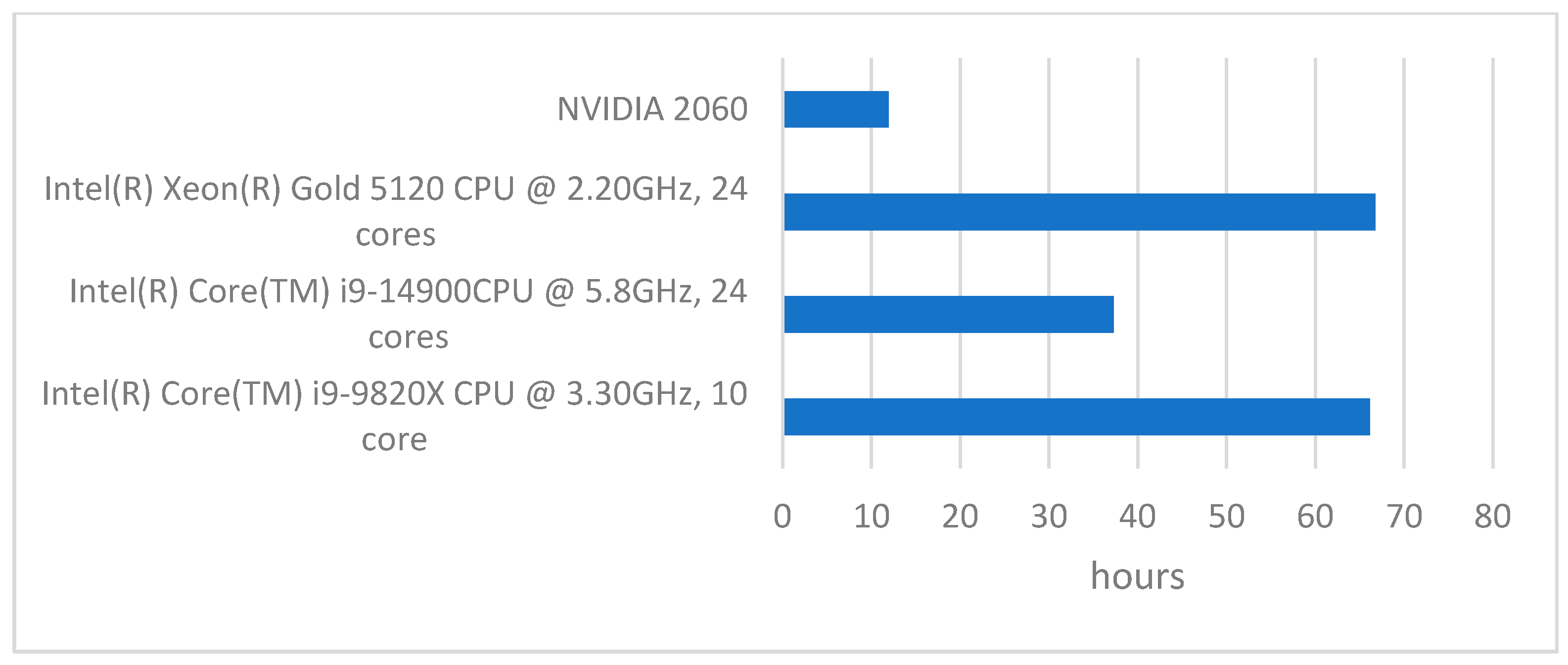
High-Performance Computing (HPC) refers to the use of powerful computing resources to solve complex problems that require significant processing power [28,29,30]. HPC systems leverage parallel computing, high-speed networks, and optimized hardware architectures to perform large-scale simulations, deep learning tasks, and scientific computations efficiently. To this end, a benchmarking study was conducted to highlight the importance of HPC for future AI-training processes. The CNN model was developed on an i9 with 24 cores, an i9 with 10 cores, a Xeon Gold with 24 cores, and an NVIDIA 2060 GPU (TSMC, Taiwan).

The benchmarking results show a clear advantage of using a GPU for CNN-based FEM surrogate modeling. The NVIDIA 2060 completed the task in just 11.95 h, significantly outperforming all tested CPUs. This was expected, as GPUs are designed for parallel computation, making them highly efficient for deep learning workloads. Among the CPUs, the Intel Core i9-14900 delivered the best performance, finishing the task in 37.32 h. Its combination of 24 cores and a high clock speed of 5.8 GHz allows it to process data much faster than the other processors. In contrast, the Intel Xeon Gold 5120 (Intel Corporate, USA), despite having the same number of cores (24), performed almost twice as slowly, taking 66.79 h.

This is due to its lower clock speed of 2.20 GHz, which limits its ability to process tasks quickly, despite the high core count. The Intel Core i9-9820X, with 10 cores and a clock speed of 3.30 GHz, performed similarly to the Xeon Gold 5120, taking 66.15 h to complete the task. This suggests that while more cores can improve calculations, clock speed plays a crucial role in overall performance, especially for deep learning workloads that require fast data processing. Overall, these results highlight the importance of using GPUs for CNN-based simulations, as even a mid-range GPU like the NVIDIA 2060 far surpasses high-end CPUs in efficiency. If a GPU is not available, a CPU with a higher clock speed, like the i9-14900, is the best alternative. However, for large-scale computation, relying on CPU processing alone would result in significantly longer execution times. The results are summarized in Figure 8.

4. Conclusions

This study has successfully demonstrated the potential of Convolutional Neural Network (CNN) surrogate models to significantly enhance the computational efficiency of finite element analyses in the nuclear fuel domain. By integrating advanced AI techniques, this study effectively reduced the computational time required for high-fidelity simulations by several orders of magnitude. The main results are as follows:

• The CNN model achieves a simulation speed that is approximately 17 times faster than traditional finite element analysis (FEA), reducing the computation time from 17 s per simulation to about 1 s.
• The CNN model maintains low Mean Squared Error (MSE) rates: the MSE for von Mises stress predictions in the best-performing setups was as low as 0.000678, indicating a high level of accuracy
• The integration of High-Performance Computing (HPC) was crucial for managing the extensive computation required for training and deploying the CNN models: the NVIDIA 2060 GPU completed the training tasks in just 11.95 h, a substantial improvement over the Intel Core i9-9820X CPU, which took approximately 66.15 h for the same tasks.

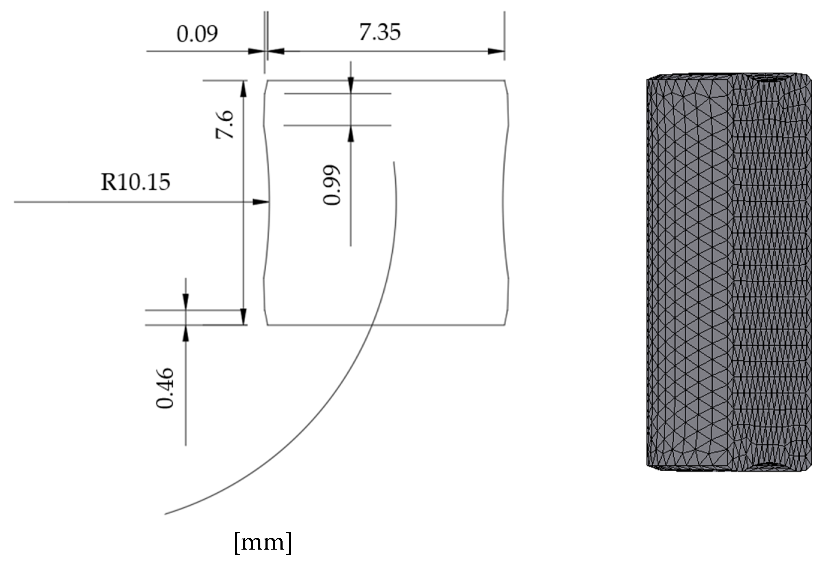
Even though the code developed shows good performance, improvements still need to be made. Currently, it is still in early development and has limitations. At this development stage, it only takes pressure as changing input. Also, the edges of the mesh (white fields in Figure 2) are converted to global minimum values, and for this reason, the user must manually identify which areas are not part of the mesh.

In the future, continuous development efforts are required to refine this model. This includes enhancing the model’s capability to automatically recognize and interpret complex geometries and conditions within the simulation environment. By overcoming these challenges, the model can be fully integrated into the operational frameworks of NPPs, ensuring effective deployment in real-world scenarios.

References

1. Cancemi, S.A.; Lo Frano, R. Inverse heat conduction problem in estimating nuclear power plant piping performance. ASME J. Nucl. Radiat. Sci. 2022, 8, 034501. [Google Scholar] [CrossRef]
2. Messner Mark, C. Convolutional Neural Network Surrogate Models for the Mechanical Properties of Periodic Structures. J. Mech. Des. 2020, 142, 024503. [Google Scholar] [CrossRef]
3. Cancemi, S.A.; Lo Frano, R. Anomalies detection in structures, system, and components for supporting nuclear long term operation program. In Proceedings of the ASME International Conference on Nuclear Engineering (ICONE29), Shenzhen, China, 8–12 August 2022. [Google Scholar] [CrossRef]
4. Cancemi, S.A.; Lo Frano, R. Unsupervised anomaly detection in pressurized water reactor digital twins using autoencoder neural networks. Nucl. Eng. Des. 2023, 413, 112502. [Google Scholar] [CrossRef]
5. Cancemi, S.A.; Angelucci, M.; Chierici, A.; Paci, S.; Lo Frano, R. Hybrid Neural Network and Statistical Forecasting Methodology for Predictive Monitoring and Residual Useful Life Estimation in Nuclear Power Plant Components. Nucl. Eng. Des. 2025, 433, 113900. [Google Scholar] [CrossRef]
6. Frazier, W.E.; Fu, Y.; Li, L.; Devanathan, R. Dynamic data-driven multiscale modeling for predicting the degradation of a 316L stainless steel nuclear cladding material. J. Nucl. Mater. 2025, 603, 155429. [Google Scholar] [CrossRef]
7. Ju, B.-S.; Son, H.-Y.; Lee, J. Advanced Sobol sensitivity analysis of a 1:4-scale prestressed concrete containment vessel using an ANN-based surrogate model. Nucl. Eng. Technol. 2025, 57, 103259. [Google Scholar] [CrossRef]
8. Wang, D.; Chen, W.; Zhu, Y.; Zhang, Y.; Fang, Y. An improved lump mass stick model of a nuclear power plant based on the Kriging surrogate model. Nucl. Eng. Des. 2024, 423, 113182. [Google Scholar] [CrossRef]
9. Hao, Y.; Wang, J.; Lin, M.; Gong, M.; Zhang, W.; Wu, B.; Ma, T.; Wang, H.; Liu, B.; Li, Y. Hybrid surrogate model-based multi-objective lightweight optimization of spherical fuel element canister. Energies 2023, 16, 3587. [Google Scholar] [CrossRef]
10. Ramancha, M.K.; Vega, M.A.; Conte, J.P.; Todd, M.D.; Hu, Z. Bayesian model updating with finite element vs surrogate models: Application to a miter gate structural system. Eng. Struct. 2022, 272, 114901. [Google Scholar] [CrossRef]
11. Khuwaileh, B.A.; Turinsky, P.J. Surrogate based model calibration for pressurized water reactor physics calculations. Nucl. Eng. Technol. 2017, 49, 1219–1225. [Google Scholar] [CrossRef]
12. Fox Mason, A.; Lindsay, I.O.; Gorton, J.P.; Brown, N.R. Reactivity-Initiated Accidents in Two Pressurized Water Reactor High Burnup Core Designs. Nucl. Eng. Des. 2024, 415, 112745. [Google Scholar] [CrossRef]
13. Reymond, M.; Sercombe, J.; Scolaro, A. Investigation of the PCMI Failure of Pre-Hydrided Zy-4 Cladding during Reactivity Initiated Accidents with ALCYONE and OFFBEAT Fuel Performance Codes. Nucl. Eng. Des. 2024, 427, 113430. [Google Scholar] [CrossRef]
14. Xie, J.; He, N.; Wang, Q.; Zhang, T. LWR Fission Gas Behavior Modeling Using OpenFOAM Based Fuel Performance Solver OFFBEAT. In Proceedings of the 2023 Water Reactor Fuel Performance Meeting, Xi’an, China, 17–21 July 2023; Liu, J., Jiao, Y., Eds.; Springer Nature: Singapore, 2024; Volume 299, pp. 251–260. [Google Scholar] [CrossRef]
15. Lucuta, P.; Matzke, H.; Hastings, I. A Pragmatic Approach to Modelling Thermal Conductivity of Irradiated UO2 Fuel: Review and Recommendations. J. Nucl. Mater. 1996, 232, 166–180. [Google Scholar] [CrossRef]
16. Izonin, I.; Tkachenko, R.; Shakhovska, N.; Ilchyshyn, B.; Singh, K.K. A Two-Step Data Normalization Approach for Improving Classification Accuracy in the Medical Diagnosis Domain. Mathematics 2022, 10, 1942. [Google Scholar] [CrossRef]
17. Browne, M.W. Cross-Validation Methods. J. Math. Psychol. 2000, 44, 108–132. [Google Scholar] [CrossRef] [PubMed]
18. Badrinarayanan, V.; Kendall, A.; Cipolla, R. SegNet. A Deep Convolutional Encoder-Decoder Architecture for Image Segmentation. IEEE Trans. Pattern Anal. Mach. Intell. 2017, 39, 2481–2495. [Google Scholar] [CrossRef] [PubMed]
19. Venkataraman, P. Image Denoising Using Convolutional Autoencoder. arXiv 2022, arXiv:2207.11771. [Google Scholar] [CrossRef]
20. Team, K. Keras Documentation: Dense Layer. Available online: https://keras.io/api/layers/core_layers/dense/ (accessed on 10 January 2025).
21. tf.keras.layers.ReLU|TensorFlow v2.16.1. Available online: https://www.tensorflow.org/api_docs/python/tf/keras/layers/ReLU (accessed on 10 January 2025).
22. TensorFlow. tf.keras.layers.Reshape|TensorFlow v2.16.1. Available online: https://www.tensorflow.org/api_docs/python/tf/keras/layers/Reshape (accessed on 10 January 2025).
23. tf.keras.layers.Resizing|TensorFlow v2.16.1. Available online: https://www.tensorflow.org/api_docs/python/tf/keras/layers/Resizing (accessed on 10 January 2025).
24. TensorFlow. tf.transpose|TensorFlow v2.16.1. Available online: https://www.tensorflow.org/api_docs/python/tf/transpose (accessed on 10 January 2025).
25. Python Release Python 3.10.0. Available online: https://www.python.org/downloads/release/python-3100/ (accessed on 10 January 2025).
26. TensorFlow. Available online: https://www.tensorflow.org/ (accessed on 10 January 2025).
27. Anaconda|Built to Advance Open Source AI. Available online: https://www.anaconda.com/ (accessed on 10 January 2025).
28. Hodson, T.O.; Over, T.M.; Foks, S.S. Mean Squared Error, Deconstructed. J. Adv. Model. Earth Syst. 2021, 13, e2021MS002681. [Google Scholar] [CrossRef]
29. Hussin, M.; Affendi, M.R.N.; Hasan, D. A Study of the High-Performance Computing Parallelism in Solving Complexity of Meteorology Data and Calculations. J. Adv. Res. Appl. Sci. Eng. Technol. 2024, 54, 16–26. [Google Scholar] [CrossRef]
30. Dan, A.; Patil, U.; De, A.; Manuraj, B.N.M.; Ramachandran, R. CPU and GPU Based Acceleration of High-Dimensional Population Balance Models via the Vectorization and Parallelization of Multivariate Aggregation and Breakage Integral Terms. Comput. Chem. Eng. 2025, 196, 109037. [Google Scholar] [CrossRef]
Figure 1. Two-dimensional and three-dimensional fuel pellet models.
Energies 18 02557 g001
Figure 2. Examples of (a) displacement, (b) creep strain, and (c) von Mises stress. Images taken from the top-down view of the mesh. Here, the red color indicates the highest value and blue represents the lowest value.
Energies 18 02557 g002
Figure 3. Examples of (a) displacement, (b) creep strain, and (c) von Mises stress. Images taken from the left-side view of the mesh. Here, the red color indicates the highest value and blue represents the lowest value.
Energies 18 02557 g003
Figure 4. Architecture of CNN model. Here, N (neurons) and Nfilters are numbers obtained from hyperparameter optimization, and can be different for each model.
Energies 18 02557 g004
Figure 5. Average von Mises stress based on testing dataset images (left case). The values have been normalized and are shown in the form of a heat colormap.
Energies 18 02557 g005
Figure 6. Predicted average von Mises stress based on testing dataset images (left case). The values have been normalized and are shown in the form of a heat colormap.
Energies 18 02557 g006
Figure 7. The difference between the predicted average and real average von Mises (left) values output by the model based on the entire testing dataset. The values been normalized and are shown in the form of a heat colormap.
Energies 18 02557 g007
Figure 8. Benchmarking of training process for CNN model.
Energies 18 02557 g008