Article

Generalized Predictive Control for a Single-Phase, Three-Level Voltage Source Inverter

1
Departamento de Ciencias Exáctas, Universidad de las Fuerzas Armadas ESPE, Sangolquí P.O. Box 171-5-231B, Ecuador
2
Departamento de Eléctrica, Electrónica y Telecomunicaciones, Universidad de las Fuerzas Armadas ESPE, Sangolquí P.O. Box 171-5-231B, Ecuador
3
Unidad de Sistemas Eléctricos, IMDEA Energía, Avda. Ramón de la Sagra, 3 Parque Tecnológico de Móstoles, 28935 Móstoles, Spain
4
Departamento de Electrónica, Universidad de Alcalá de Henares, 28801 Alcalá de Henares, Spain
5
Department of Electrical Engineering, ESAT, KU Leuven-EnergyVille, 3590 Diepenbeek, Belgium
*
Authors to whom correspondence should be addressed.
Energies 2025, 18(10), 2541; https://doi.org/10.3390/en18102541
Submission received: 4 April 2025 / Revised: 9 May 2025 / Accepted: 11 May 2025 / Published: 14 May 2025
(This article belongs to the Section F3: Power Electronics)

Abstract

:
In recent years, the study of model predictive control (MPC) in power electronics has gained significant attention due to its ability to optimize system performance and improve the dynamic control of complex power converters. There are two types of MPC: finite control set (FCS) and continuous control set (CCS). The FCS–MPC has been studied more in regard to these two types of control due to its easy and intuitive implementation. However, FCS–MPC has some drawbacks, such as the exponential growth of the computational burden as the prediction horizon increases and, in some cases, a variable frequency. In contrast, generalized predictive control (GPC), part of CCS–MPC, offers significant advantages. It enables the use of a longer prediction horizon without increasing the computational burden in regard to its implementation, which has practical implications for the efficiency and performance of power converters. This paper presents the design of GPC applied to single-phase multilevel voltage source inverters, highlighting its advantages over FCS–MPC. The controller is optimized offline, significantly reducing the computational cost of implementation. Moreover, the controller is tested in regard to R, RL, and nonlinear loads. Finally, the validation results using a medium-performance controller and a Hardware-in-the-Loop device highlight the improved behavior of the proposed GPC, maintaining a harmonic distortion of less than 1.2% for R and RL loads.

1. Introduction

Worldwide, the demand for electric power is growing exponentially each year [1], prompting the search for new, environmentally friendly energy sources that reduce the carbon footprint [2]. Thus, renewable energy sources (RESs) have been critical to this research [3]. Photovoltaic (PV) energy is a type of RES that is currently being widely studied. It is a long-term alternative sustainable energy source, due to its low environmental impact [4]. However, PV systems produce a direct current (DC), whereas most loads worldwide demand an alternating current (AC). For this reason, it is necessary to use DC/AC converters [5].
Voltage source inverters (VSIs) can operate in two modes: connected to the grid or stand-alone [6]. In the grid-connected operating mode, the VSI injects current into the grid. In this case, the voltage should be controlled and synchronized with the grid voltage. Additionally, the power factor and total harmonic distortion (THD) must be maintained within the optimum values specified by the mains [7]. Conversely, in stand-alone operating mode, the VSI is responsible for setting the voltage signal for the isolated grid. In this case, the voltage signal and its harmonic content must be controlled to provide a higher quality power source for customers [8]. Although grid-connected VSIs have been more widely studied, VSI applications in regard to stand-alone systems have increased in recent years, particularly in ground, air, and sea vehicles, wherein many of these systems are considered autonomous [9].
VSIs may have two or more voltage levels at their output. When they have more than two voltage levels, they are known as multilevel VSIs. Compared to two-level VSIs, multilevel VSIs enable a significant reduction in the THD in the voltage waveform to be achieved as the voltage levels increase [10]. Several configurations of multilevel VSIs include a cascade flying capacitor, a H-bridge, and a neutral-point-clamped (NPC) topology. Each of these topologies has its own specific benefits and characteristics [11]. However, the T-type NPC VSI configuration has become a topology of great interest, mainly due to its simple structure and the reduced number of power devices it utilizes. Additionally, it produces lower losses, thereby improving both thermal and electrical efficiency compared to other NPC configurations [12].
Several control strategies applied to multilevel VSIs have been extensively studied in the last few years [13]: fuzzy logic control [14,15], deadbeat (DB) control [16,17], PID control [18], sliding mode control [19,20], and model predictive control (MPC) [21,22], among others. However, MPC has become the most relevant and studied control technique, as it outperforms other control techniques [23]. Two groups of MPC can be distinguished: finite control set MPC (FCS–MPC) and continuous control set MPC (CCS–MPC). Both strategies utilize the system’s mathematical model to predict its performance and a cost function to minimize the error between the set point and the control input [21]. On the one hand, although the number of control inputs limits FCS–MPC, it has been studied more extensively than CCS–MPC, mainly due to its intuitive implementation and the ease of incorporating constraints. Additionally, this control strategy emphasizes online optimization, resulting in increased computational costs. In addition, it presents some drawbacks when implemented, such as issues with the filter design and a variable control frequency, which cause an increase in THD, an exponential increase in the computational burden as the prediction horizon increases, and an increase in power switch losses [24]. On the other hand, CCS–MPC has several advantages over FCS–MPC, including the absence of input limitations in the controller, continuous control signals, and an external modulator, which results in a fixed control frequency. In this way, the VSI operates at an optimal energy efficiency point, allowing the output filter to be designed for improved THD management [25].
Generalized predictive control (GPC) is a technique that belongs to the CCS–MPC family, which has gained increasing interest in regard to power electronics applications in recent years, such as in regard to power converters and motor control [26,27]. GPC utilizes the system’s mathematical representation, which is defined by the plant transfer function. Additionally, the disturbance model of GPC enhances the rejection of external disturbances in the closed-loop system. GPC utilizes a quadratic cost function, focusing on minimizing the control effort to ensure that the future plant output aligns with the reference value. For this reason, the cost function minimizes the error between the set point and the plant output and the increment in the system’s control action [28,29]. From this perspective, the system can be optimized offline without considering the constraints, significantly reducing the computational cost and eliminating the arduous work involved in online optimization [25].
Several studies have been conducted on GPC in power electronics. For instance, the authors in [30] employ an ARMAX–GPC controller in an energy management system between multiple energy sources in a microgrid, aiming to minimize the cost of the energy consumed as a result of the load. The authors in [31] propose the application of GPC to the grid-side converter of a wind turbine. This work aims to track the variable power as a function of the nominal frequency deviation, wherein the control achieves a faster return to the nominal frequency than when FCS–MPC is applied. In addition, the study presented in [32] develops a methodology for controlling both active and non-active instantaneous power based on GPC, which enables the control of grid-connected converter performance under grid disturbances. The authors in [25] utilize GPC to control the current of a boost converter. This work performs cost function optimization offline, considerably reducing the control strategy’s computation time to less than 5 µs. Additionally, the results showed that GPC is more robust than a PI controller and a proportional–resonant (PR) controller. Moreover, in [33], a control system consisting of two GPC control loops is proposed. The outer loop controls the DC voltage, whereas the inner loop controls the AC source current. However, synthesizing the two control loops into one enables a reduction in the computational cost to be achieved. In [34], an active disturbance rejection controller uses the modified GPC cost function to generate an optimal control action. This control approach is applied to a three-phase grid-connected VSI, reducing the computational cost through offline optimization. Additionally, the authors in [35] consider a GPC cost function optimized offline to determine the optimal voltage for a three-phase VSI. This study achieves the optimum voltage vector form, which is applied using space vector modulation, converting the control into FCS–MPC. In addition, the authors in [36] propose the use of a generalized predictive controller (GPC) in the natural reference frame for a three-phase LCL filter-based grid-tied inverter. This controller achieves high accuracy in regulating active and reactive currents, demonstrates robustness in regard to variations in grid inductance, requires minimal real-time computational effort, and operates with a fixed switching frequency.
Furthermore, in the works described in [37,38], the authors focused on developing a GPC-based control strategy optimized offline and applied to a grid-connected three-phase, two-level VSI. On the one hand, the authors in [37] employ an L filter, a prediction horizon of eight, and a control horizon of five, achieving a total harmonic distortion (THD) of 2.7%. On the other hand, although both horizons are increased in [38], the THD of 3.91% remains unchanged because the plant becomes more complex when using an LCL filter. The authors in [39] also develop GPC for a single-phase full-bridge VSI, utilizing an online parametric identification method to determine the plant coefficients. Although this work achieves a low THD implementation, the control is not tested under non-linear loads (NLs). Finally, on the one hand, the study described in [40] presents GPC, coupled with a repetitive controller, applied to a grid-connected inverter. This hybrid control aims to decrease the harmonics in the current caused by a distorted grid voltage. On the other hand, the study in [41] presents GPC coupled with resonant control for tracking voltage signals, thereby overcoming disturbances in a maximum time of 6.4 ms. However, the designed control exhibits a significant peak in the voltage signal, which can cause damage to switching devices.
Thus, after analyzing previous works, it is concluded that GPC is an attractive, efficient, and robust control method used in power converters. However, this control strategy remains scarcely studied in multilevel VSIs disconnected from the grid, so the field of research in regard to this control strategy is open. Similarly, it has been observed that multilevel converters significantly reduce the THD produced in regard to the current and voltage of the VSI. In this regard, as an extension of the research developed in [42], this study focuses on developing a voltage control methodology based on generalized predictive control (GPC) applied to a T-type NPC VSI disconnected from the mains. This proposal uses an orthogonal signal generator that enables the Park transformation to be achieved. This way, the controller input will correspond to the amplitude of the voltage generated by the VSI, allowing for a faster response to system dynamics compared to RMS-based control. Additionally, the cost function optimization is performed offline, enabling the integration of an orthogonal signal generator (OSG), the Park transformation, and GPC within a microcontroller. Finally, the effectiveness of the proposed control is validated by implementing GPC in a Texas Instruments (Dallas, TX, USA) F28335 microcontroller and the T-type NPC VSI in a Typhoon Hardware-in-the-Loop HIL402 device (Typhoon HIL d.o.o., Novi Sad, Serbia).
The main contributions of this work are as follows:
  • A proposal for a GPC controller applied to a multilevel VSI in off-grid operation mode;
  • CCS–MPC real-time implementation with a vast prediction horizon, without increasing the computational cost;
  • A complete integration of the entire control strategy within a single control device, eliminating the need for additional filters or intermediate devices.
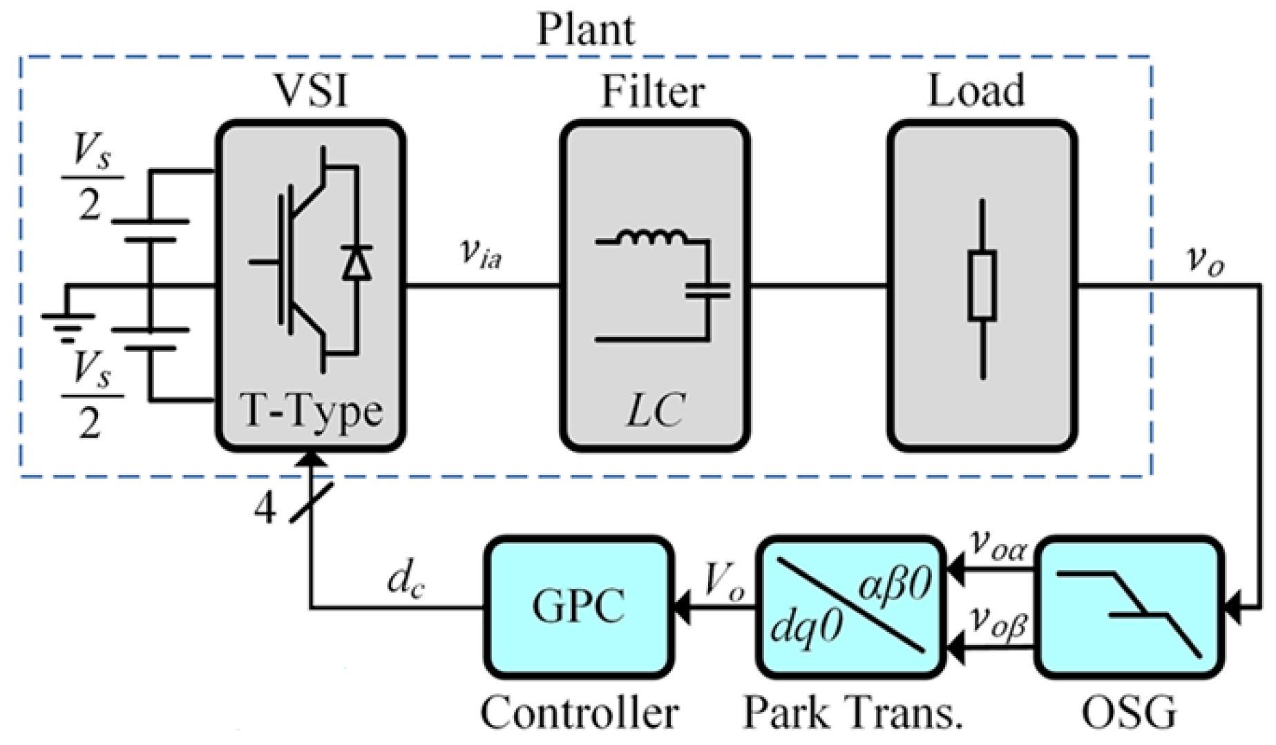
The rest of the paper is organized as follows: Section 2 describes the analysis of the mathematical model of the single-phase T-type NPC VSI. Section 3 compares the proposed system’s simulation process with a PI controller. Section 4 presents the controller and VSI’s real-time implementation results. Finally, Section 5 summarizes the main conclusions of this research and outlines future work.

2. System Modeling

The system primarily consists of a GPC controller and a DC/AC converter. However, since it is a single-phase system, additional tools, such as an OSG and a Park transformation block, are required to obtain an equivalent voltage signal to control it. Figure 1 summarizes the control loop proposed in this research. The components used in this control system are explained below.

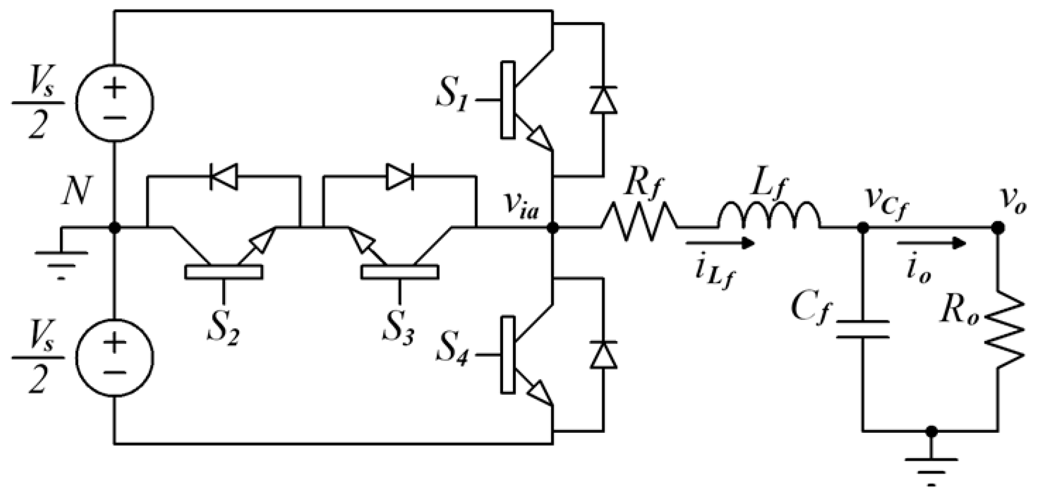
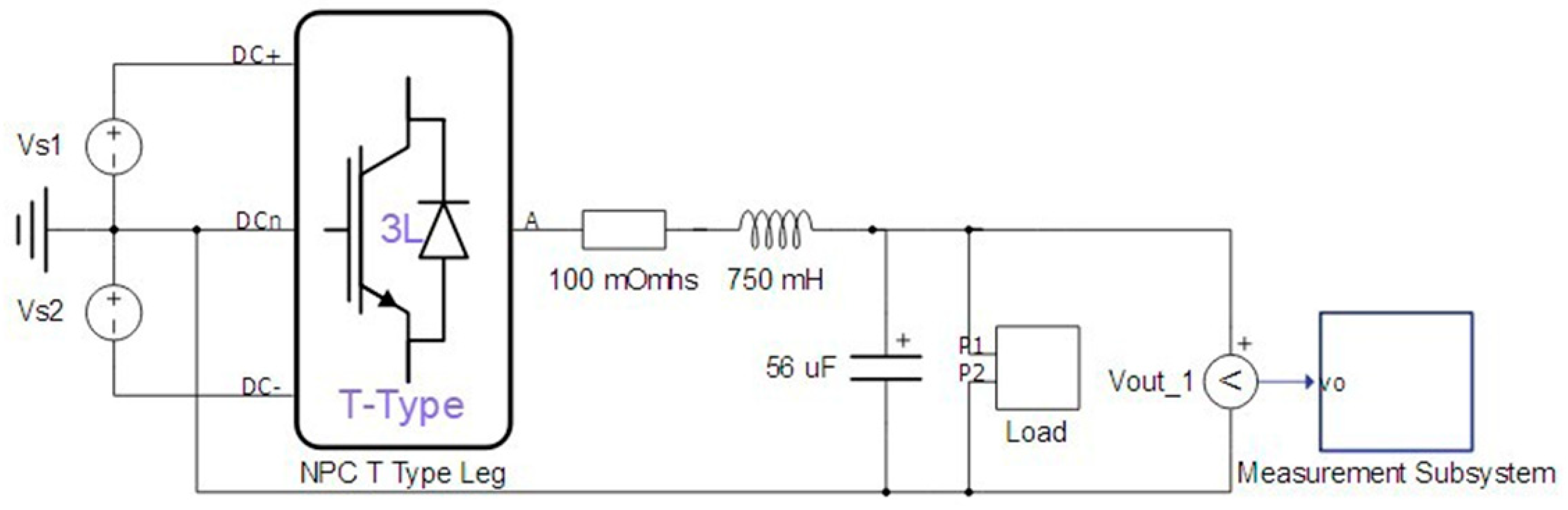
2.1. Single-Phase T-Type NPC Voltage Source Inverter

A multilevel DC/AC converter generates various voltage levels on the AC link. The more levels present at the output of a VSI, the closer the voltage will be to a sine wave. Therefore, the harmonic content of a multilevel inverter is lower than that of a traditional two-level inverter [43]. Several configurations of multilevel inverters exist. However, the T-type NPC configuration stands out from the others due to its high efficiency and the optimized number of switching devices used [44,45]. In this regard, this work uses a three-level T-type NPC VSI, as shown in Figure 2.
The T-type NPC configuration shown in Figure 2 comprises four switches, S1 and S3 having complementary signals, as do S2 and S4. Thus, Table 1 details three possible state (u) combinations, where 1 and 0 represent the ON and OFF states, respectively. Figure 3 presents the corresponding circuits and current flow for each state.
Table 1 and Figure 3 show that each combination provides a different voltage level. Filters connected to a VSI output reduce the high-frequency harmonic content in the voltage signal [46]. In this case, an LC filter is used at the inverter’s output. The filter comprises an inductor (Lf) with losses represented by the resistance Rf, and a capacitor (Cf) connected in parallel, as shown in Figure 2. In addition, a load (Ro) is connected to the filter output. Note that the voltage applied to the load (vo) is the same as the voltage on the capacitor (vCf); iLf corresponds to the current flowing through the inductor and io is the current supplied to the load. In this regard, the state–space of the T-type NPC VSI, which represents the mathematical system model in terms of time t, is detailed in Equation (1), as follows:
i L F d t v C f d t = R f L f 1 L f 1 C f 1 R o C f i L f v C f + 1 L f 0 v i a v o = 0 1 i L f v C f
Based on the system’s state–space model, the transfer function that determines the relationship between vo and via is computed by Equation (2), as follows:
G p ( s ) = 1 L f C f s 2 + s R f L f + 1 R o C f + R o + R f R o L f C f

2.2. Orthogonal Signal Generator

Three-phase systems utilize Clarke and Park transformations to convert AC signals into their equivalent representations in an orthogonal frame [47]. On the one hand, the Clarke transformation converts three-phase systems based on abc coordinates to a stationary orthogonal reference frame based on αβ0 coordinates. Several control systems use these vector coordinates to control electric machines and converters [48]. On the other hand, the Park transformation converts αβ0 coordinates to a rotating orthogonal reference frame based on dq0 coordinates. Using these two transformations generates a signal whose value is equal to the amplitude of the original signal. This resulting signal facilitates the processing of the controller’s input data [49].
However, single-phase systems only have a unique AC signal. Therefore, several studies have been conducted to apply these transformations to these systems [50,51,52]. An orthogonal signal generator (OSG) is employed to achieve this, which produces a quadrature signal relative to the original AC signal. Thus, both signals generate a system based on αβ0 coordinates, making it possible to perform the Park transformation in regard to a single-phase system. The difference between RMS-based control and control relating to a rotating orthogonal frame is embodied in a faster response to the system’s dynamics. Due to its high performance and low computational cost, this work uses a second-order filter-based OSG, as shown in Figure 4 [53].
In Figure 4, ωn and ξ are the undamped natural frequency and the damping ratio, respectively. In this case, ξ = 1, and ωn equals the natural frequency of the voltage. The voltage signal vo corresponds to the signal voα, and the filter’s output corresponds to the signal voβ. Both components are the input signals in regard to Park’s transformation block, as detailed in Figure 1, wherein the output signals are the direct voltage (vd), whose value corresponds to the voltage amplitude of vo (Vo), and the quadrature voltage (vq).

2.3. Generalized Predictive Control

GPC is a control technique based on the controlled autoregressive integrated moving average (CARIMA) model. This form of control has been extensively described in [28,29]. In this regard, at the current sampling instant t, the output prediction for a single-input–single-output (SISO) system can be modeled using Equation (3), as follows:
A ( z 1 ) y ( t ) = B ( z 1 ) z d u c ( t 1 ) + C c ( z 1 ) e ( t ) 1 z 1
where z−1 is the backward shift operator, A and B are the plant’s polynomial denominator and numerator, respectively, y(t) is the plant’s output, uc is the control action, Cc(z−1) is a polynomial to improve the rejection of load disturbance inputs, and e(t) is the zero-mean white noise. Note that in the case of non-stationary disturbances, Cc(z−1) is set to 1, and the control action of GPC will be equivalent to the modulator duty cycle value (dc).
GPC generates an optimal control action considering both the control horizon (Nc) and the prediction horizon (Np). This controller uses a cost function (J), expressed in Equation (4), that minimizes the increment in the control action (Δuc) and the error between the optimal prediction of the system output y ^ (t + j|t) j steps ahead in terms of the data up to time t and the reference ω, as follows [28]:
J N p , N c = j = 1 N p δ ( j ) y ^ ( t + j | t ) ω ( t + j ) 2 + j = 1 N c λ ( j ) Δ u c ( t + j 1 ) 2
where δ and λ are the weights of the prediction and control components, respectively. Note that the optimization is achieved by solving the Diophantine Equation (5). As a result, the control action optimal increment is computed as follows [29]:
Δ u c ( t ) = K ( w f )
where K is the proportional control action applied to the error between the reference vector (w) and the system’s free response (f); both K and f values are obtained by solving the Diophantine equation. Readers may refer to [28] for a more detailed mathematical analysis.
The proposed control system corresponds to CCS–MPC with a long prediction horizon. Most of the controllers in the literature correspond to FCS–MPC and are based on three-phase grid-connected systems. In contrast to other controllers, the proposed controller is specifically designed for an isolated single-phase VSI and is distinguished by its lower computational cost.

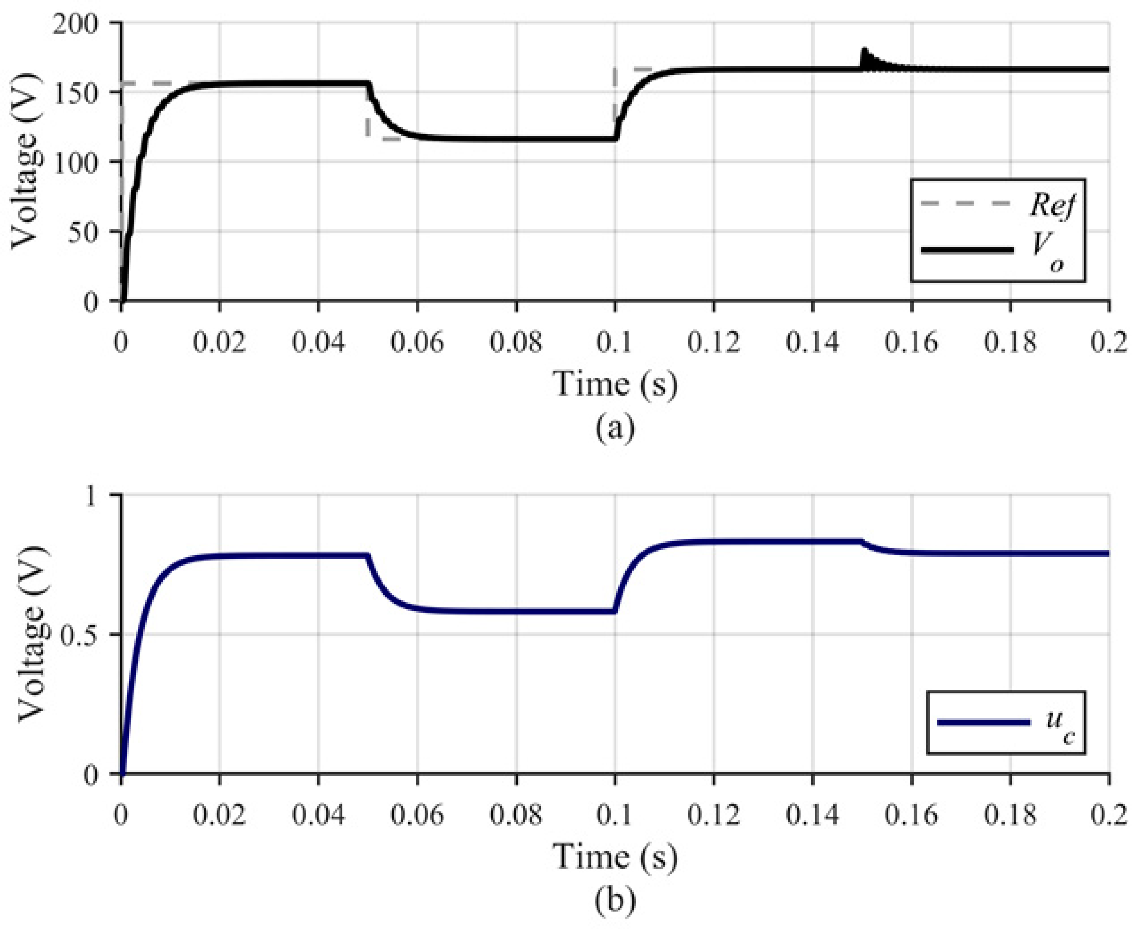
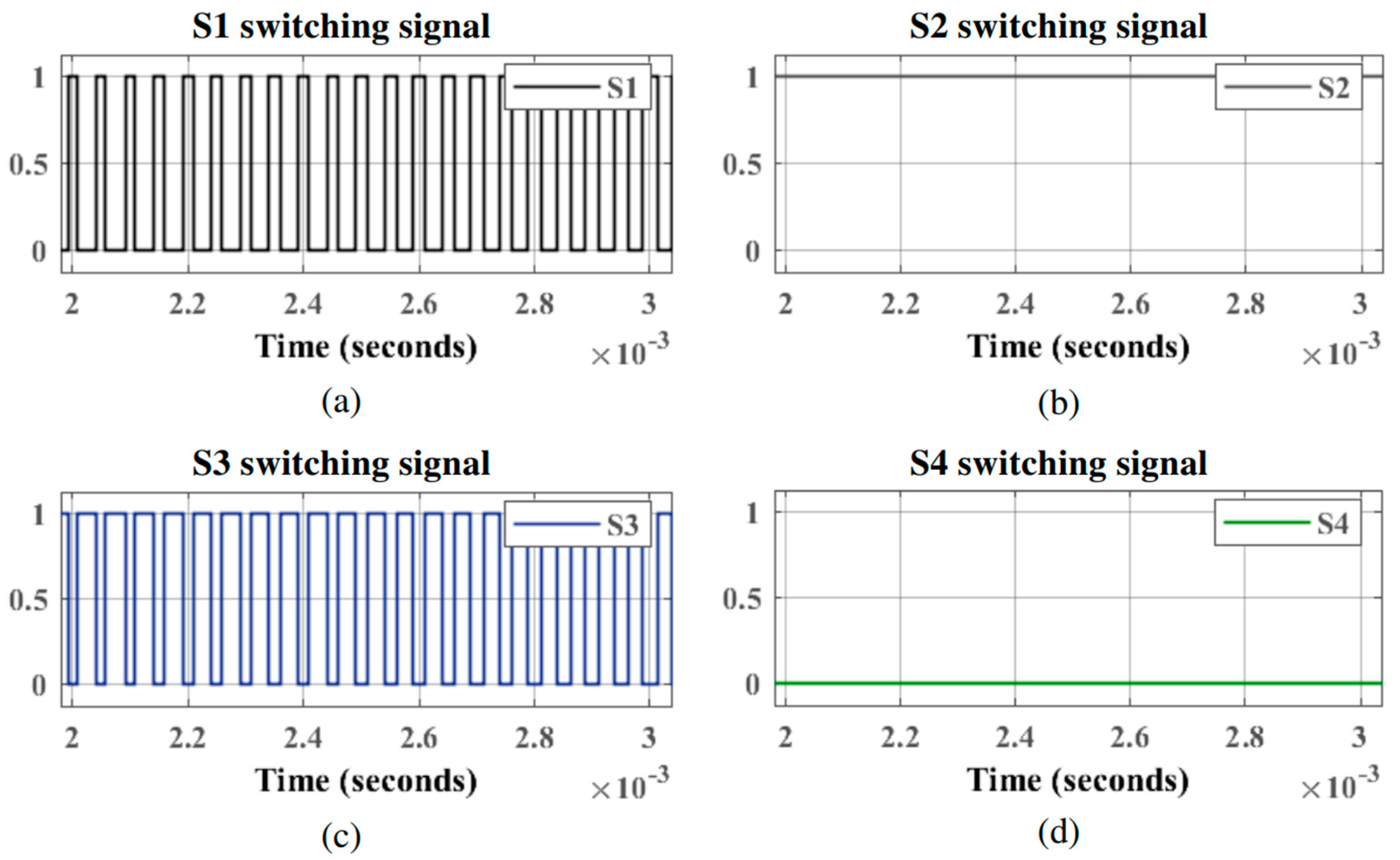
3. Simulation Results

Table 2 presents the simulation parameters used in this study. These parameters are based on a previous study detailed in [42]. Therefore, considering (2), the system’s discretized transfer function, using the ZOH method, at 50 µs is defined in Equation (6), as follows:
G p ( z ) = 0.02933 z 1 + 0.02905 z 2 1 1.91290 z 1 + 0.97143 z 2
The controller cost function parameters are tuned offline for simulation purposes, whereas the GPC algorithm is implemented in Matlab® R2023a. This study assumes that the values Np and Nc are equal (Np = Nc = N), the system has no delays (d = 0), and the value δ is set to 1. Since the response with a higher speed and a control action with fewer harmonics is achieved with values of N ≥ 9 [35], a value of N = 9 is considered, as no better performance could be obtained with more extended control and prediction horizons. Additionally, the computational cost of implementing the control algorithm increases as the value of N increases. In this regard, Figure 5 shows the system performance as a function of the weighting factor λ.
As shown in Figure 5, the weighting factor λ adjusts the system’s stabilization time. The higher this value, the slower the system response and the smoother the control action in the transient state. Conversely, the lower the value of λ, the faster the system responds to disturbances. However, the transient response is more dynamic, producing significantly more harmonics during this transition. Therefore, to select the value λ, a settling time (tst) of 20 ms has been considered for the system. Thus, the value λ that fulfills the design requirements, i.e., to achieve a response without a high level of harmonic content and to comply with the proposed tst, is obtained by trial and error (λ = 390).
Figure 6 presents the plant’s performance using the proposed GPC, illustrating the control loop’s response to set-point changes and system output disturbances. The reference is modified for simulation at 50 and 100 ms, whereas a perturbation is added to the system output at 150 ms. In both cases, the controller takes less than 20 ms to get the system to its reference value. Additionally, Figure 6 illustrates that the control action enables smooth adjustments in the system in response to changes in the reference and external perturbations.
In this regard, the control loop detailed in Figure 1 is implemented online, using MATLAB® Simulink. For the simulation and design, a Core i7-9750H computer with six processors, a clock of 2.60 GHz, 32 GB RAM, and an RTX 2070 graphics card is used.
GPC values found and optimized offline are considered for this procedure. Additionally, a PI controller with a parallel architecture is implemented to compare the simulation results obtained with the proposed GPC.
Figure 7 and Figure 8 show the control output of the GPC corresponding to the switching states of switches S1, S2, S3, and S4, at different time intervals. As detailed in Table 1, the T-type NPC configuration has three possible switching combinations between the switches representing the three output voltage levels. Unlike a two-level inverter, the T-type NPC configuration enables the reconstruction of the output signal with lower harmonic content. Figure 7 represents the reconstruction of the output voltage between 0 and +Vs/2, wherein S2 stays high and S4 stays low, while S1 and S3 switch inversely. Similarly, Figure 8 shows the reconstruction of the voltage output between −Vs/2 and 0, wherein S3 stays high and S1 stays low, while S2 and S4 switch inversely.
One way to determine the improvement in the output of a T-type NPC VSI inverter is to determine the harmonic content of the output signal, which is accomplished by applying Fast Fourier Transform (FFT) [54]. FFT decomposes a periodic signal into sinusoidal components, with different frequencies, amplitudes, and phases. It is a fundamental component of and involves a series of harmonics generated by the inverter’s switching. FFT itself provides the frequency spectrum of the inverter’s output signal. This spectrum is utilized to measure the distortion at the inverter’s output [55]. Total harmonic distortion has been used to measure each controller’s performance in regard to the inverter. THD quantifies the harmonic distortion of the voltage signal at the inverter output (vo) and indicates the presence of multiple harmonic components of the fundamental frequency [56]. A low THD indicates an efficient control system and a vo signal closer to a sine wave. THD is computed using (7) as follows:
T H D ( % ) = h = 2 h max V H , h V H , 1 2 100
where VH,1 is the root mean square (RMS) voltage of the fundamental frequency component, and VH,h represents the sum of the RMS voltages of all the harmonic components. The gain values of the PI controller (i.e., Kp = 0.0025 and Ki = 1.5) are tuned to achieve a response with a settling time (tst) of less than 20 ms, without overshoot, and with a THD of less than 5%.
As detailed in [35], controller behavior is analyzed by measuring the resulting THD under three load scenarios, connected to the LC filter output. The first scenario uses resistive loads, the second uses RL loads, and the third uses NL loads, based on a wave rectifier with a parallel RC output load. These results are detailed in Table 3, Table 4 and Table 5.
On the one hand, from the results in Table 3 and Table 4, voltage signals with different R and RL loads exhibit a THD of less than 2.6%. Conversely, the PI controller fails to control the systems with low resistive loads and high inductance values for RL loads, resulting in system instability. On the other hand, both controllers show an increase in the THD as the NL load increases, as detailed in Table 5. GPC maintains a THD of less than 8% for low-power NL loads and performs better than the PI controller. In contrast, for higher power NL loads, the PI controller performs better; however, both controllers exceed the maximum value of 8% recommended in [57] for systems with a voltage below 1 kV. It is worth mentioning that GPC can handle the R, RL, and some NL loads, even though these types of loads were not considered during the design process.
Moreover, Figure 9 illustrates the response of both controllers to various load disturbances. The simulation considers an initial load of 50 Ω and a disturbance, connected in parallel to the load at 0 ms. Figure 9a–c presents the response to a resistive load disturbance of 20 Ω, an RL load disturbance (R = 50 Ω and L = 20 mH), and an NL load disturbance, based on a full-wave rectifier with a parallel RC load (R = 200 Ω and C = 330 μF), respectively.
As shown in Figure 9a,b (i.e., resistive and RL load disturbances), GPC exhibits similar behavior to the PI controller, achieving a voltage signal with a low THD in the transient state. Conversely, regarding NL loads, as shown in Figure 9c, both controllers exhibit significant oscillations before following the reference value. However, GPC controls the situation faster than the PI controller, maintaining system stability at less than 20 ms. Additionally, GPC produces a lower THD during the transient stage than the PI controller. The simulation results highlight the improved performance of the proposed GPC compared to the PI controller. In this regard, the following Section presents the real-time implementation of the proposed control system.

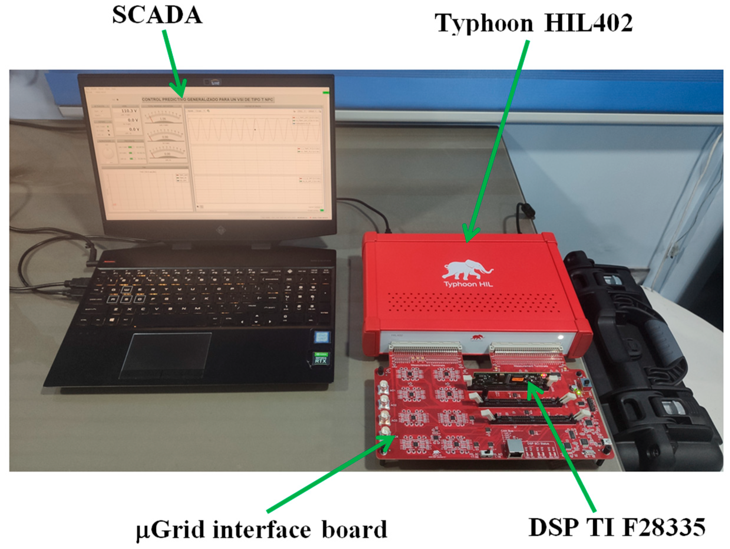
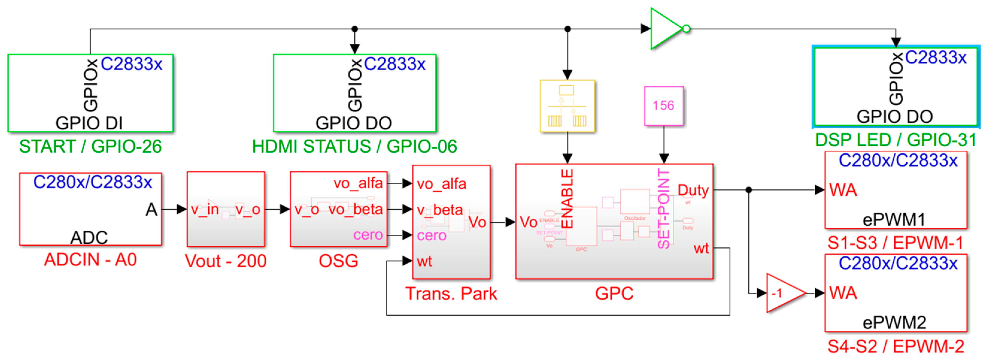
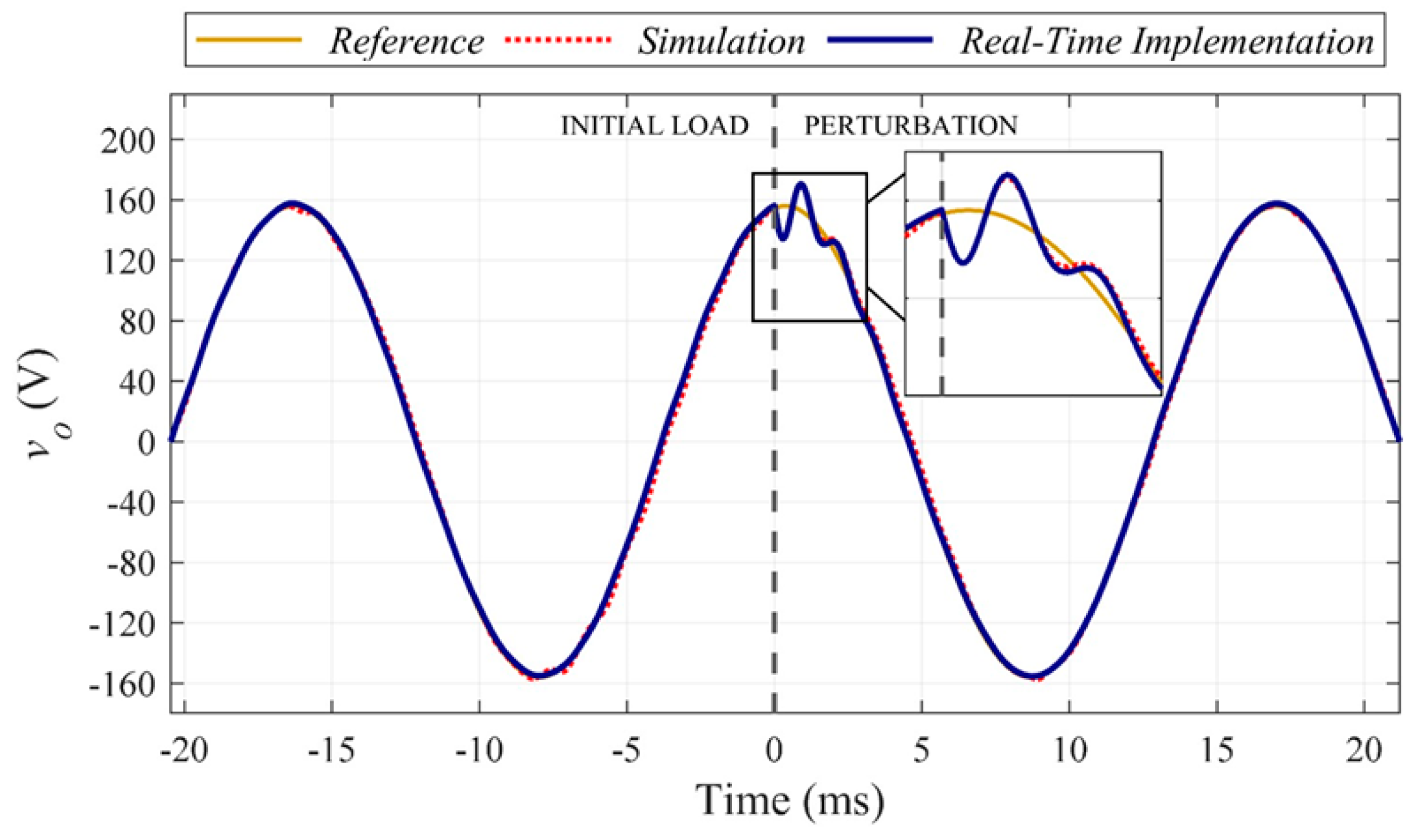
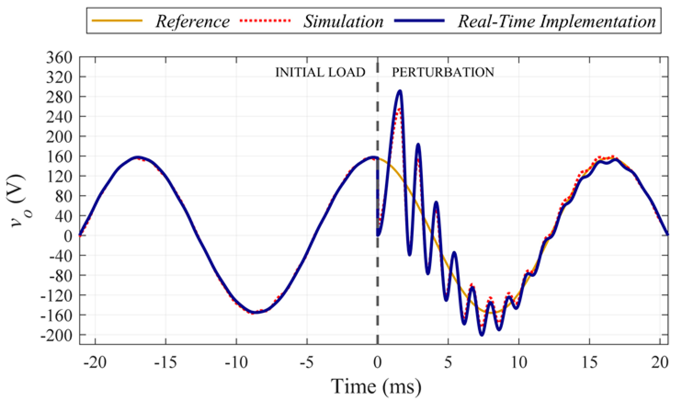
4. System Implementation and Results

The control loop depicted in Figure 1 is implemented to test the real-time operation of the proposed GPC controller. This study utilizes a Hardware-in-the-Loop (HIL) Typhoon HIL402 device and a Texas Instruments F28335 DSP to implement the system’s plant, a filtered T-type NPC VSI, and the proposed GPC controller, respectively. Moreover, a Typhoon HIL μGrid interface connects the DSP to the Typhoon HIL 402 device. Additionally, a local computer’s SCADA interface is configured to retrieve data and measurements from the control loop, as illustrated in Figure 10.
Figure 11 shows the HIL’s plant implementation scheme. The plant consists of two DC sources (Vs1 and Vs2), a T-type NPC VSI, an LC filter, according to the values specified in Table 2, and a load connected to the filter’s output. Moreover, a measurement system is added to send the voltage signal to the DSP through an analog output. Likewise, this measurement system enables tracking of the plant’s main variables, such as the voltage (vo), THD, and frequency. An exact discretization method and a simulation step of 0.5 μs are used for the compilation process.
Figure 12 presents the flowchart for embedding the controller in the DSP. An analog-to-digital input (ADCIN-A0), a digital input (GIPO-26), and two complementary pulse-width modulation (PWM) outputs (ePWM-1 and ePWM-2) are utilized. First, the ADCIN-A0 allows the reading of the voltage vo, which has been scaled (1:40) according to the HIL402 analog output. Then, the GPIO-26 activates the algorithm through a signal generated by the SCADA system. Finally, the control output is transduced to a duty cycle variation and sent to the ePWM outputs.
The controller is programmed in the DSP, using the embedded encoder support package in Simulink for Texas Instruments C2000 processors, to generate optimized code. In this sense, the system is simulated in Simulink, and the changes are made to direct the control outputs to the ePWM1 and ePWM2 outputs. Similarly, the ADCIN-A0 input is configured to read the voltage signal and form the closed control loop. Figure 13 shows the program embedded in the DSP, corresponding to the controller detailed in this work.
As shown in Figure 13, ePWM1 and ePWM2 outputs use complementary outputs and are driven to control switches S1, S2, S3, and S4. Additionally, the GPIO-26 input externally activates the control system, and the GPIO-06 and GPIO-31 outputs correspond to indicators on the Typhoon HIL HDMI and DSP, respectively.
It is worth mentioning that since the GPC parameters are obtained offline, only (5) is considered for the controller implementation. Thus, this study assumes that the K value is constant and time invariant. The system is tested under the three scenarios described in Section 3 to evaluate the performance of the proposed GPC in a real-time environment. The comparison of the resulting THDs achieved through the simulation and in a real-time environment for the three scenarios is summarized in Table 6, Table 7 and Table 8. Notice that the real-time tests are performed for 5 min, and the values detailed in these tables represent the average value achieved during this time interval.
As shown in Table 6, Table 7 and Table 8, the results obtained in a real-time environment are similar to those from the simulation. However, they differ mainly due to dynamics not considered in the simulation process and their impact on real-time system performance. The results obtained for the first scenario, corresponding to resistive loads, indicate a maximum THD of 1.02%. As shown in Table 6, the THD increases as the resistance value increases. Similarly, the results for the second scenario, which corresponds to RL loads (see Table 7), show a maximum THD of 1.15%. In this case, the THD increases as the inductance value increases. However, a THD of less than 8% is maintained in both scenarios, the maximum recommended by [48]. Finally, the results for the last scenario, corresponding to NL loads (see Table 8), show an increase in the THD as the load value increases. This is due to the nature of NL loads and their impact on the grid current, which distorts the voltage signal and increases the THD. It is worth mentioning that although the system has not been designed to control NL loads, the GPC can control low-power NL loads.
Additionally, the same three load disturbance scenarios described in Section 3 demonstrate the effectiveness of the proposed GPC. Figure 14 presents the results obtained from the simulation and real-time tests, wherein the system is perturbed with a load of 20 Ω.
As shown in Figure 14, the real-time test results for an R load disturbance are similar to those obtained in the simulation. When the disturbance load is connected, the system presents a peak voltage of 170 V, which returns to a steady state due to the GPC controller. This disturbance is handled in less than 4 ms. Figure 15 displays the simulation and real-time results in response to RL load disturbance (R = 50 Ω and L = 20 mH).
Similarly, the real-time test results for an RL disturbance are close to those obtained in the simulation, as seen in Figure 15. The system experiences less impact for this load than the R load disturbance, mainly due to the inductive effect of the load, which acts as an additional filter and mitigates the more aggressive effect of the disturbance. No peak voltage is present in this scenario, and the load disturbance is controlled at 3 ms. Finally, the results achieved in the third scenario are depicted in Figure 16.
The effect of these oscillations causes a high level of harmonic content during approximately one cycle of the voltage waveform. The highest peak value is 291.3 V, representing a variation of 86.7% in the peak voltage value (156 V). In contrast, the lowest peak value is 0 V, equivalent to a 100% variation from the peak voltage value. Despite this, the system returns to a steady state after 18.5 ms. This effect is primarily due to the nature of the NL load, which generates a high level of harmonic content in the network. Finally, it is essential to emphasize that although the controller is not specifically designed to regulate NL loads, it can effectively control disturbances caused by this type of load.

5. Conclusions

This paper presents a novel control strategy based on generalized predictive control applied to a single-phase multilevel T-type NPC VSI. An OSG based on a second-order low-pass filter has been used to generate a system in a rotating orthogonal reference frame, where the controller input is the peak voltage of the sinusoidal signal generated by the VSI. The GPC controller has been optimized offline. After several tests, a prediction and control window involving nine steps was selected, as the control system did not show a considerable improvement beyond this value. In addition, the simulation results show improvements over those achieved by a classical PI controller, wherein the PI controller fails to control the voltage signal in response to some of the tested loads. GPC decreased the THD steadily and controlled the situation effectively, with a faster response achieved during the transient state in the analyzed scenarios. In this regard, the VSI was simulated in real-time using a Typhoon HIL402 device, whereas the entire control system, including the OSG, Park transformation, and GPC, was implemented on an F28335 DSP board. As a result, the embedded control algorithm requires 30 µs in order to calculate the control output. The results saw GPC achieve a maximum THD of 1.2% for linear loads (R and RL). Finally, the proposed controller managed the R and RL disturbances in less than 4 ms, whereas the NL disturbance was achieved in less than 18 ms. The results obtained in a real-time environment demonstrated the effectiveness of the proposed GPC controller applied to a single-phase multilevel T-type NPC VSI.
To strengthen the proposed approach, our future work will consider the following:
  • An experimental validation and efficiency analysis of the proposed approach involving a real T-type NPC VSI;
  • Apply restrictions to the GPC cost function and improve the control technique for NL loads;
  • Perform a comprehensive study of various metaheuristic and machine learning methods for controlling a T-type NPC VSI.

Author Contributions

Conceptualization, P.A. and D.A.-A.; methodology, P.A. and D.N.; software, D.N.; validation, D.N., P.A., J.A., W.M., and D.A.-A.; formal analysis, D.N., J.A., and P.A.; investigation, D.N.; resources, D.N. and J.A.; data curation, D.N.; writing—original draft preparation, D.N., P.A., J.A. and D.A.-A.; writing—review and editing, D.N., P.A., J.A., W.M. and D.A.-A.; visualization, D.A.-A.; supervision, P.A.; project administration, D.A.-A.; funding acquisition, D.A.-A. All authors have read and agreed to the published version of the manuscript.

Funding

This work is part of project 2024-PIM-05 by the Research Group of Propagation, Electronic Control, and Networking (PROCONET) at the Universidad de las Fuerzas Armadas ESPE.

Data Availability Statement

The data presented in this study are available on request from the corresponding author.

Conflicts of Interest

The authors declare that there are no conflicts of interest.

References

  1. International Energy Agency. World Energy Outlook 2022; International Energy Agency: Paris, France, 2022. [Google Scholar]
  2. Meral, M.E.; Çelík, D. A comprehensive survey on control strategies of distributed generation power systems under normal and abnormal conditions. Annu. Rev. Control 2019, 47, 112–132. [Google Scholar] [CrossRef]
  3. Memon, M.A.; Mekhilef, S.; Mubin, M.; Aamir, M. Selective harmonic elimination in inverters using bio-inspired intelligent algorithms for renewable energy conversion applications: A review. Renew. Sustain. Energy Rev. 2018, 82, 2235–2253. [Google Scholar] [CrossRef]
  4. Sultana, W.R.; Sahoo, S.K.; Sukchai, S.; Yamuna, S.; Venkatesh, D. A review on state of art development of model predictive control for renewable energy applications. Renew. Sustain. Energy Rev. 2017, 76, 391–406. [Google Scholar] [CrossRef]
  5. Mohamed, A.A.S.; Metwally, H.; El-Sayed, A.; Selem, S.I. Predictive neural network based adaptive controller for grid-connected PV systems supplying pulse-load. Sol. Energy 2019, 193, 139–147. [Google Scholar] [CrossRef]
  6. Silva, F.A. Advanced DC\/AC Inverters: Applications in Renewable Energy. IEEE Ind. Electron. Mag. 2013, 7, 68–69. [Google Scholar] [CrossRef]
  7. Amin, M.R.; Zulkifli, S.A. A framework for selection of grid-inverter synchronisation unit: Harmonics, phase-angle and frequency. Renew. Sustain. Energy Rev. 2017, 78, 210–219. [Google Scholar] [CrossRef]
  8. Andishgar, M.H.; Gholipour, E.; Hooshmand, R. An overview of control approaches of inverter-based microgrids in islanding mode of operation. Renew. Sustain. Energy Rev. 2017, 80, 1043–1060. [Google Scholar] [CrossRef]
  9. Khooban, M.-H. Secondary Load Frequency Control of Time-Delay Stand-Alone Microgrids With Electric Vehicles. IEEE Trans. Ind. Electron. 2018, 65, 7416–7422. [Google Scholar] [CrossRef]
  10. Hassan, A.; Yang, X.; Chen, W.; Houran, M.A. A State of the Art of the Multilevel Inverters with Reduced Count Components. Electronics 2020, 9, 1924. [Google Scholar] [CrossRef]
  11. Rana, R.A.; Patel, S.A.; Muthusamy, A.; Lee, C.W.; Kim, H.-J. Review of Multilevel Voltage Source Inverter Topologies and Analysis of Harmonics Distortions in FC-MLI. Electronics 2019, 8, 1329. [Google Scholar] [CrossRef]
  12. Aly, M.; Ahmed, E.M.; Shoyama, M. Modulation Method for Improving Reliability of Multilevel T-Type Inverter in PV Systems. IEEE J. Emerg. Sel. Top. Power Electron. 2020, 8, 1298–1309. [Google Scholar] [CrossRef]
  13. Trabelsi, M.; Alquennah, A.N.; Vahedi, H. Review on Single-DC-Source Multilevel Inverters: Voltage Balancing and Control Techniques. IEEE Open J. Ind. Electron. Soc. 2022, 3, 711–732. [Google Scholar] [CrossRef]
  14. Basha, S.G.; Mani, V.; Mopidevi, S. Single-phase thirteen-level dual-boost inverter based shunt active power filter control using resonant and fuzzy logic controllers. CSEE J. Power Energy Syst. 2020, 8, 849–863. [Google Scholar] [CrossRef]
  15. Das, S.R.; Mishra, A.K.; Sahoo, A.K.; Hota, A.P.; Viriyasitavat, W.; Alghamdi, N.S.; Dhiman, G. Fuzzy Controller Designed-Based Multilevel Inverter for Power Quality Enhancement. IEEE Trans. Consum. Electron. 2024, 70, 4839–4847. [Google Scholar] [CrossRef]
  16. Trabelsi, M.; Ben-Brahim, L.; Gastli, A.; Abu-Rub, H. Enhanced Deadbeat Control Approach for Grid-Tied Multilevel Flying Capacitors Inverter. IEEE Access 2022, 10, 16720–16728. [Google Scholar] [CrossRef]
  17. Ramaiah, S.L.N.; Mishra, M.K. Loss Modulated Deadbeat Control for Grid Connected Inverter System. IEEE J. Emerg. Sel. Top. Power Electron. 2023, 11, 3715–3725. [Google Scholar] [CrossRef]
  18. Stonier, A.A.; Murugesan, S.; Samikannu, R.; Venkatachary, S.K.; Kumar, S.S.; Arumugam, P. Power Quality Improvement in Solar Fed Cascaded Multilevel Inverter With Output Voltage Regulation Techniques. IEEE Access 2020, 8, 178360–178371. [Google Scholar] [CrossRef]
  19. Makhamreh, H.; Trabelsi, M.; Kukrer, O.; Abu-Rub, H. An Effective Sliding Mode Control Design for a Grid-Connected PUC7 Multilevel Inverter. IEEE Trans. Ind. Electron. 2020, 67, 3717–3725. [Google Scholar] [CrossRef]
  20. Anssari, O.M.H.; Badamchizadeh, M.; Ghaemi, S. Designing of a PSO-Based Adaptive SMC With a Multilevel Inverter for MPPT of PV Systems Under Rapidly Changing Weather Conditions. IEEE Access 2024, 12, 41421–41435. [Google Scholar] [CrossRef]
  21. Andino, J.; Ayala, P.; Llanos-Proano, J.; Naunay, D.; Martinez, W.; Arcos-Aviles, D. Constrained Modulated Model Predictive Control for a Three-Phase Three-Level Voltage Source Inverter. IEEE Access 2022, 10, 10673–10687. [Google Scholar] [CrossRef]
  22. Huo, X.; Li, P. Parameter-free ultralocal model-based predictive current control method for grid-tied inverters using extremum seeking control. Control Eng. Pract. 2025, 157, 106253. [Google Scholar] [CrossRef]
  23. Azizi, A.; Akhbari, M.; Danyali, S.; Tohidinejad, Z.; Shirkhani, M. A review on topology and control strategies of high-power inverters in large- scale photovoltaic power plants. Heliyon 2025, 11, e42334. [Google Scholar] [CrossRef] [PubMed]
  24. Cheng, L.; Acuna, P.; Aguilera, R.P.; Jiang, J.; Wei, S.; Fletcher, J.E.; Lu, D.D. Model Predictive Control for DC–DC Boost Converters With Reduced-Prediction Horizon and Constant Switching Frequency. IEEE Trans. Power Electron. 2018, 33, 9064–9075. [Google Scholar] [CrossRef]
  25. Judewicz, M.G.; González, S.A.; Fischer, J.R.; Martínez, J.F.; Carrica, D.O. Generalised predictive current-mode control of passive front-end boost-type converters. IET Power Electron. 2021, 14, 666–679. [Google Scholar] [CrossRef]
  26. De Oliveira, H.A.; Torrico, B.C.; De, S.D.; Barbosa, S.G.; De Almeida Filho, M.P. Predictive Control Applied to a Single-Stage, Single-Phase Bidirectional AC-DC Converter. IEEE Access 2022, 10, 34984–34995. [Google Scholar] [CrossRef]
  27. Shao, M.; Deng, Y.; Li, H.; Liu, J.; Fei, Q. Robust Speed Control for Permanent Magnet Synchronous Motors Using a Generalized Predictive Controller With a High-Order Terminal Sliding-Mode Observer. IEEE Access 2019, 7, 121540–121551. [Google Scholar] [CrossRef]
  28. Camacho, E.F.; Bordons, C. Generalized Predictive Control. In Model Predictive Control of Microgrids. Advances in Industrial Control, 2nd ed.; Springer: London, UK, 2007; Volume 4, pp. 47–79. [Google Scholar] [CrossRef]
  29. Bordons, C.; Garcia-Torres, F.; Ridao, M.A. Microgrids Power Quality Enhancement. In Model Predictive Control of Microgrids. Advances in Industrial Control, 2nd ed.; Springer: London, UK, 2020. [Google Scholar] [CrossRef]
  30. Franco, R.A.P.; Cardoso, Á.A.; Filho, G.L.; Vieira, F.H.T. MIMO auto-regressive modeling-based generalized predictive control for grid-connected hybrid systems. Comput. Electr. Eng. 2022, 97, 107636. [Google Scholar] [CrossRef]
  31. Cerón, C.E.P.; Lourenço, L.F.N.; Solís-Chaves, J.S.; Filho, A.J.S. A Generalized Predictive Controller for a Wind Turbine Providing Frequency Support for a Microgrid. Energies 2022, 15, 2562. [Google Scholar] [CrossRef]
  32. Šimek, P.; Valouch, V. Generalized predictive power control for grid-connected converter. Int. J. Electr. Power Energy Syst. 2021, 125, 106380. [Google Scholar] [CrossRef]
  33. Wang, T.; Zhu, Z.Q.; Freire, N.M.A.; Stone, D.A.; Foster, M.P. Generalized Predictive dc-Link Voltage Control for Grid-Connected Converter. IEEE J. Emerg. Sel. Top. Power Electron. 2022, 10, 1489–1506. [Google Scholar] [CrossRef]
  34. Tran, T.V.; Kim, K.-H.; Lai, J.-S. Optimized Active Disturbance Rejection Control With Resonant Extended State Observer for Grid Voltage Sensorless LCL -Filtered Inverter. IEEE Trans. Power Electron. 2021, 36, 13317–13331. [Google Scholar] [CrossRef]
  35. Lunardi, A.; Conde, D.E.R.; de Assis, J.; Fernandes, D.A.; Filho, A.J.S. Model Predictive Control with Modulator Applied to Grid Inverter under Voltage Distorted. Energies 2021, 14, 4953. [Google Scholar] [CrossRef]
  36. Zamani, H.; Abbaszadeh, K.; Karimi, M.; Gyselinck, J. Offset free generalized model predictive control for 3-phase LCL-filter based grid-tied inverters. Int. J. Electr. Power Energy Syst. 2023, 153, 109351. [Google Scholar] [CrossRef]
  37. Judewicz, M.G.; Gonzalez, S.A.; Echeverria, N.I.; Fischer, J.R.; Carrica, D.O. Generalized Predictive Current Control (GPCC) for Grid-Tie Three-Phase Inverters. IEEE Trans. Ind. Electron. 2016, 63, 4475–4484. [Google Scholar] [CrossRef]
  38. Judewicz, M.G.; Gonzalez, S.A.; Fischer, J.R.; Martinez, J.F.; Carrica, D.O. Inverter-Side Current Control of Grid-Connected Voltage Source Inverters With LCL Filter Based on Generalized Predictive Control. IEEE J. Emerg. Sel. Top. Power Electron. 2018, 6, 1732–1743. [Google Scholar] [CrossRef]
  39. Memeghani, M.J.; Ghamari, S.M.; Jouybari, T.Y.; Mollaee, H.; Wheeler, P. Generalised predictive controller (GPC) design on single-phase full-bridge inverter with a novel identification method. IET Control Theory Appl. 2023, 17, 284–294. [Google Scholar] [CrossRef]
  40. Lunardi, A.; Conde, E.; Assis, J.; Meegahapola, L.; Fernandes, D.A.; Filho, A.J.S. Repetitive Predictive Control for Current Control of Grid-Connected Inverter Under Distorted Voltage Conditions. IEEE Access 2022, 10, 16931–16941. [Google Scholar] [CrossRef]
  41. Cordero, R.; Estrabis, T.; Brito, M.A.; Gentil, G. Development of a Resonant Generalized Predictive Controller for Sinusoidal Reference Tracking. IEEE Trans. Circuits Syst. II Express Briefs 2022, 69, 1218–1222. [Google Scholar] [CrossRef]
  42. Naunay, D.; Ayala, P.; Andino, J.; Martinez, W.; Llanos, J.; Arcos-Aviles, D. Generalized predictive control strategy applied to a single-phase T-type voltage source inverter in stand-alone operation mode. In Proceedings of the 22nd Workshop on Control and Modelling of Power Electronics (COMPEL), Cartagena, Colombia, 2–5 November 2021; pp. 1–7. [Google Scholar] [CrossRef]
  43. Boussada, Z.; Elbeji, O.; Benhamed, M. Modeling of diode clamped inverter using SPWM technique. In Proceedings of the International Conference on Green Energy Conversion Systems (GECS), Hammamet, Tunisia, 23–25 March 2017; pp. 1–5. [Google Scholar] [CrossRef]
  44. Prabaharan, N.; Palanisamy, K. A comprehensive review on reduced switch multilevel inverter topologies, modulation techniques and applications. Renew. Sustain. Energy Rev. 2017, 76, 1248–1282. [Google Scholar] [CrossRef]
  45. Sebaaly, F.; Kanaan, H.Y.; Moubayed, N. Three-level neutral-point-clamped inverters in transformerless PV systems—State of the art. In Proceedings of the MELECON 2014—2014 17th IEEE Mediterranean Electrotechnical Conference, Beirut, Lebanon, 13–16 April 2014; pp. 1–7. [Google Scholar] [CrossRef]
  46. Mishra, P.; Maheshwari, R. Design, Analysis, and Impacts of Sinusoidal LC Filter on Pulsewidth Modulated Inverter Fed-Induction Motor Drive. IEEE Trans. Ind. Electron. 2020, 67, 2678–2688. [Google Scholar] [CrossRef]
  47. Zou, Y.; Zhang, L.; Xing, Y.; Zhang, Z.; Zhao, H.; Ge, H. Generalized Clarke Transformation and Enhanced Dual-Loop Control Scheme for Three-Phase PWM Converters Under the Unbalanced Utility Grid. IEEE Trans. Power Electron. 2022, 37, 8935–8947. [Google Scholar] [CrossRef]
  48. O’Rourke, C.J.; Qasim, M.M.; Overlin, M.R.; Kirtley, J.L. A Geometric Interpretation of Reference Frames and Transformations: dq0, Clarke, and Park. IEEE Trans. Energy Convers. 2019, 34, 2070–2083. [Google Scholar] [CrossRef]
  49. Tan, G.; Sun, X. Analysis of Tan-Sun Coordinate Transformation System for Three-Phase Unbalanced Power System. IEEE Trans. Power Electron. 2018, 33, 5386–5400. [Google Scholar] [CrossRef]
  50. Bamigbade, A.; Khadkikar, V.; Zeineldin, H.H.; El Moursi, M.S.; Al Hosani, M. A Novel Power-Based Orthogonal Signal Generator for Single-Phase Systems. IEEE Trans. Power Deliv. 2021, 36, 469–472. [Google Scholar] [CrossRef]
  51. Bertoluzzo, M.; Giacomuzzi, S.; Kumar, A. Design and Experimentation of a Single-Phase PLL With Novel OSG Method. IEEE Access 2022, 10, 33393–33407. [Google Scholar] [CrossRef]
  52. Kang, Y.G.; Reigosa, D.D. Improving Harmonic Rejection Capability of OSG Based on n-th Order Bandpass Filter for Single-Phase System. IEEE Access 2021, 9, 81728–81739. [Google Scholar] [CrossRef]
  53. Lamo, P.; Pigazo, A.; Azcondo, F.J. Evaluation of Quadrature Signal Generation Methods with Reduced Computational Resources for Grid Synchronization of Single-Phase Power Converters through Phase-Locked Loops. Electronic 2020, 9, 2026. [Google Scholar] [CrossRef]
  54. Madgula, S.; Veeramsetty, V.; Durgam, R. Signal processing approaches for power quality disturbance classification: A comprehensive review. Results Eng. 2025, 25, 104569. [Google Scholar] [CrossRef]
  55. Chen, W.; Bazzi, A.M. Model-Based Voltage Quality Analysis and Optimization in Post-Fault Reconfigured N-Level NPC Inverter. IEEE Trans. Power Electron. 2021, 36, 13706–13715. [Google Scholar] [CrossRef]
  56. Arranz-Gimon, A.; Zorita-Lamadrid, A.; Morinigo-Sotelo, D.; Duque-Perez, O. A Review of Total Harmonic Distortion Factors for the Measurement of Harmonic and Interharmonic Pollution in Modern Power Systems. Energies 2021, 14, 6467. [Google Scholar] [CrossRef]
  57. IEEE Std 519-2014 (Revision IEEE Std 519-1992); 519-2014—IEEE Recommended Practice and Requirements for Harmonic Control in Electric Power Systems. IEEE: Piscataway, NJ, USA, 2014; pp. 1–29. [CrossRef]
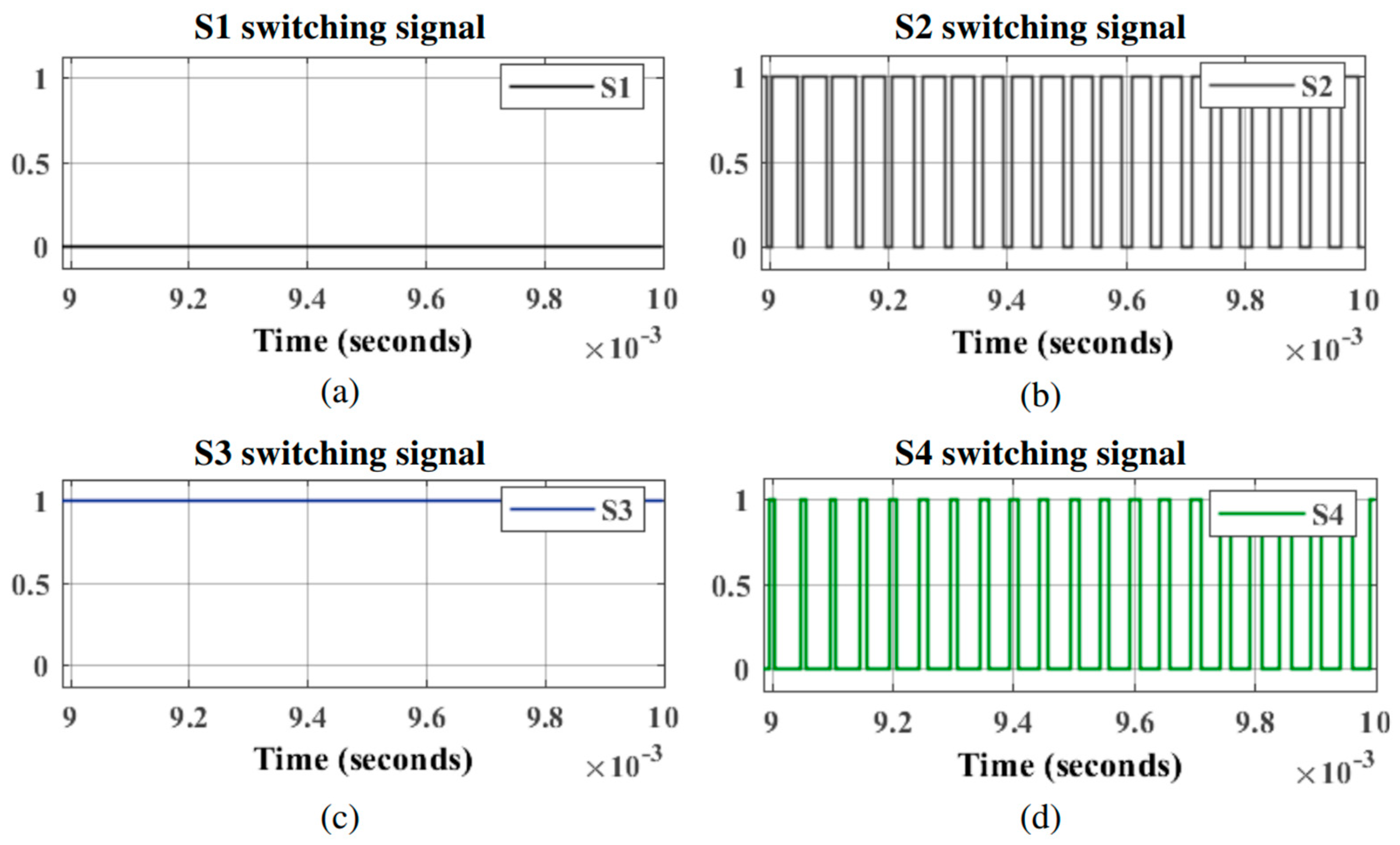
Figure 1. Proposed loop for a T-type NPC VSI, based on generalized predictive control.
Energies 18 02541 g001
Figure 2. Single-phase T-type NPC VSI.
Energies 18 02541 g002
Figure 3. Switching states and driving paths of the T-type NPC converter: (a) switching state at a high voltage (u = 1); (b) switching state at a neutral voltage (u = 0); and (c) switching state at a low voltage (u = −1).
Energies 18 02541 g003
Figure 4. Second-order filter-based OSG.
Energies 18 02541 g004
Figure 5. System response performance as a function of the weighting factor λ.
Energies 18 02541 g005
Figure 6. Performance of the system controlled by GPC with values of N = 9, δ = 1, and λ = 390: (a) reference tracking of system output Vo; and (b) GPC control action uc.
Energies 18 02541 g006
Figure 7. PWM switching signals of the inverter switches between 0 and +Vs/2: (a) S1, (b) S2, (c) S3, and (d) S4.
Energies 18 02541 g007
Figure 8. PWM switching signals of the inverter switches between −Vs/2 and 0: (a) S1, (b) S2, (c) S3, and (d) S4.
Energies 18 02541 g008
Figure 9. Response of the GPC and PI controllers to different load disturbances at t = 0 ms: (a) resistive load disturbance; (b) RL load disturbance; and (c) the NL load is based on a full-wave rectifier with a parallel RC load.
Energies 18 02541 g009
Figure 10. Interconnection between the T-type NPC VSI and the proposed GPC, implemented in regard to a Typhoon HIL402 device and DSP F28335, respectively.
Energies 18 02541 g010
Figure 11. HIL implementation scheme of the T-type NPC VSI system.
Energies 18 02541 g011
Figure 12. Flowchart of the embedded DSP program.
Energies 18 02541 g012
Figure 13. Embedded program in the DSP through the use of the Texas Instruments C2000 embedded code support package.
Energies 18 02541 g013
Figure 14. Response of the GPC T-type NPC VSI system to a resistive load disturbance.
Energies 18 02541 g014
Figure 15. Response of the GPC T-type NPC VSI system to an RL load disturbance.
Energies 18 02541 g015
Figure 16. Response of the GPC T-type NPC VSI system to an NL load disturbance.
Energies 18 02541 g016
Table 1. Switching states for a T-type NPC VSI.
uS1S2S3S4Via
11100+Vs/2
001100
−10011Vs/2
Table 2. Simulation parameters.
ParameterDefinitionValueUnit
VsDC-link voltage400V
voNominal AC-link voltage110VRMS
fnNominal frequency60Hz
fsSwitching frequency20kHz
TsSampling time50μs
LfFilter inductance750μH
RfInductance resistance100
CfFilter capacitance56μF
RoOutput load40Ω
Table 3. THD during the simulation process for different resistive loads.
ControlTHD (%)
R = 5.5 ΩR = 20 ΩR = 50 ΩR = 500 ΩR = 1000 Ω
GPC0.290.661.412.402.58
PI0.290.741.25144.27154.14
Table 4. THD during the simulation process for different RL loads.
ControlTHD (%)
Case 1
R = 50 Ω, L = 10 mH
Case 2
R = 50 Ω, L = 20 mH
Case 3
R = 50 Ω, L = 50 mH
GPC1.511.801.91
PI3.6594.02161.90
Table 5. THD during the simulation process for different NL loads, based on a wave rectifier connected to an RC output load.
ControlTHD (%)
Case 1
C = 330 μF, R = 100 Ω
Case 2
C = 330 μF, R = 200 Ω
Case 3
C = 330 μF, R = 500 Ω
GPC9.436.403.58
PI8.517.085.26
Table 6. Comparison between simulation and implementation results for different resistive loads.
GPCTHD (%)
R = 5.5 ΩR = 20 ΩR = 50 ΩR = 500 ΩR = 1000 Ω
IMP0.830.790.891.020.99
SIM0.290.661.412.402.58
Table 7. Comparison between simulation and implementation results for different RL loads.
GPCTHD (%)
Case 1
R = 50 Ω, L = 10 mH
Case 2
R = 50 Ω, L = 20 mH
Case 3
R = 50 Ω, L = 50 mH
IMP0.991.061.15
SIM1.511.801.91
Table 8. Comparison between simulation and implementation results for different NL loads, based on a wave rectifier connected to an RC output load.
GPCTHD (%)
Case 1
C = 330 μF, R = 100 Ω
Case 2
C = 330 μF, R = 200 Ω
Case 3
C = 330 μF, R = 500 Ω
IMP9.306.393.81
SIM9.436.403.58
Disclaimer/Publisher’s Note: The statements, opinions and data contained in all publications are solely those of the individual author(s) and contributor(s) and not of MDPI and/or the editor(s). MDPI and/or the editor(s) disclaim responsibility for any injury to people or property resulting from any ideas, methods, instructions or products referred to in the content.

