Numerical Assessment of Nuclear Cogeneration Transients with SMRs Using CATHARE 3–MODELICA Coupling

Abstract

To achieve the decarbonisation goal by 2050, nuclear energy can be a useful element for the future energy mix, complementing intermittent renewable sources. Additionally, heat from the core can be used for cogeneration, aiding the decarbonisation of several energy sectors. In this context, Small Modular Reactors (SMRs) are being studied when introduced in Nuclear–Renewable Hybrid Energy Systems for cogeneration applications. However, nuclear cogeneration with SMRs is still an emerging area of study, requiring careful considerations regarding technical, safety, and economic aspects. European research initiatives, such as the TANDEM project, are exploring the integration of light–water SMRs into hybrid systems. This paper investigates the impact of cogeneration transients on the primary system of an SMR using a novel coupling approach. For this scope, the thermal–hydraulic system code CATHARE 3 and the dynamic modelling language MODELICA are adopted. Three transient scenarios were analysed: cogeneration transitions, core power variations, and thermal load rejection. The results achieved provide insights about the robustness of the numerical coupling and the primary system response to cogeneration-induced transients. As a matter of fact, the analysis shows that the reactor system is mildly influenced by cogeneration changes, and the findings suggest future improvements for both the coupling methodology and modelling assumptions.

1. Introduction

In order to mitigate the severe consequences that climate change could bring to our planet if the average global temperature increases beyond 2 °C [1], 196 parties chose to sign the Paris Agreement on climate change in 2015, committing to strategies aimed at limiting the global average temperature rise to below 1.5 °C compared to pre-industrial levels [2]. To achieve this goal, a massive decarbonisation process of the energy sector must be undertaken, aiming to achieve a net-zero carbon energy mix by 2050 [3]. According to several scenarios described by the International Energy Agency (IEA) [3], a widespread adoption of renewable energy sources (RES), the electrification of different energy sectors, and an increase in the energy efficiency of the energy users would be the best pathway to achieve the net-zero goal.

Nevertheless, the envisaged increase in the electricity demand caused by both the increase in world population [4] and the electrification of some energy sectors could bring about several issues in the electricity infrastructures and more globally in energy security. Moreover, electricity production accounts for only a portion of the global carbon emissions [5], whereas there are some intensive thermal energy users, e.g., the steel industry, which are hard to decarbonise and/or to completely electrify. In this regard, the need of a stable and carbon free energy source, e.g., nuclear energy [6], could bring different benefits to the future energy mix. In particular, nuclear energy could be used to supply low carbon energy for the electricity baseload demand, thus constituting a backbone of the future electrical grid [7], helping to limit the stress induced on the grid due to a widespread adoption of intermittent energy sources. Moreover, the adoption of a stable baseload energy source would also mitigate the high grid costs needed for grid balance components (e.g., frequency control systems [8]), electricity storages, and backup sources to supply the demand during the peak hours [9].

Besides favouring the stability of the grid, nuclear energy will also help to decarbonise hard-to-abate sectors through the cogeneration of thermal power or, alternatively, to produce other valuable products. In fact, nuclear cogeneration can be used to produce thermal power at different temperature levels [10] depending on the reactor technology, which can potentially provide heat to supply civil district heating [11], water desalination plants [12], and paper production (i.e., low temperature heat). Nuclear reactors belonging to generation IV, instead, have the potential to produce thermal heat to supply different chemical industries, e.g., ammonia production [10] or high temperature electrolysis processes, which commonly require higher temperatures than the one provided by light–water reactors (LWRs). The cogeneration of thermal power, moreover, besides potentially enhancing the flexibility of the nuclear power plant by adopting a load-following strategy including cogeneration [13], could also help to mitigate other issues that are foreseen to be crucial in the future, e.g., fresh water shortages [1] and the adoption of hydrogen as fuel, aiming to decarbonise the transportation sector and some hard-to-abate industrial processes [3].

In the frame of nuclear cogeneration, Small Modular Reactors (SMRs) have gained increasing attention during the past years due to their advantages in terms of modularity, flexibility, and potentially higher safety. The use of SMRs in cogeneration environments brought about the concept of Nuclear–Renewable Hybrid Energy Systems (N-R HES) [14], in line with the scenarios envisaged by different international agencies about possible future decarbonised energy mixes [3,15]. However, hybrid energy systems pose different issues from technical, economical, and safety viewpoints, which need particular attention and assessment to facilitate their future development. For instance, the coupling between a nuclear power plant and a general heat user must be evaluated from both technical and safety standpoints. It must be demonstrated, in fact, that the safety of the nuclear source is not compromised by the adoption of cogeneration [16]. In the European research panorama, several initiatives were carried out regarding nuclear cogeneration, e.g., the EUROPAIRS [17], NC2I-R, and GEMINI [18], which focused on cogeneration with high-temperature gas reactors. Regarding light–water technology, instead, the TANDEM EURATOM project [19] aims to assess the techno-economic feasibility of adopting light–water SMR (LW SMR) in hybrid energy systems. In this regard, one of the goals of the TANDEM project is to develop tools for assessing the safety of nuclear cogeneration with LW SMRs.

In this context, the present paper describes the results of a work conducted within the framework of the TANDEM project concerning the development of a code-coupling methodology between a thermal–hydraulic system code, namely CATHARE 3 [20], and a dynamic modelling language, namely MODELICA [21], with the final goal of achieving a useful tool to perform safety analyses of nuclear cogeneration. The main idea behind the code coupling is to leverage the strengths of the two codes, i.e., the wide validation and assessment of CATHARE 3 to perform nuclear safety analyses and the great flexibility and reusability of the MODELICA language, especially when adopted to model complex systems. Being the development of a MODELICA library for N-R HES modelling one of the goals of TANDEM [19], a model of the reference design of LW SMR was developed with the CATHARE 3 code and then a coupling methodology was initially assessed between the two codes [22]. The code coupling was performed by means of the Functional Mock-up Interface (FMI) tool [23]. The present numerical coupling, performed using the commercial software Dymola 24x [24], was used to assess three meaningful transients involving nuclear cogeneration, both to assess the robustness of the coupling and to achieve preliminary information about the response of the primary system to such scenarios. The paper is structured as follows:

• Section 1 describes the two adopted models, i.e., the SMR primary circuit developed with CATHARE 3 and the BOP model belonging to the TANDEM open source MODELICA library [25,26];
• Section 3 provides information about the adopted philosophy for coupling the two codes and the numerical coupling scheme developed via Dymola 24x using the Modelica Standard Library [27];
• Section 4 describes the addressed transient scenarios and the rationale behind their choice;
• Section 5 briefly illustrates the results of the coupled analyses;
• Section 6 draws relevant conclusions and highlights the future perspectives of the work.

2. Description of the Adopted Models

In this chapter, the two models involved in the code coupling are described, aiming to sketch their general features, including the main assumptions at their basis. The reference design of SMR plant considered by the TANDEM project takes inspiration from an academic concept of LW SMR, namely the European Small Modular Reactor (ESMR), which is one of the outcomes of a former European research project called ELSMOR [28]. The BOP model, instead, is one of those belonging to the TANDEM MODELICA library [26], which includes several models, also developed in the framework of the TANDEM project, of different components of a N-R HES.

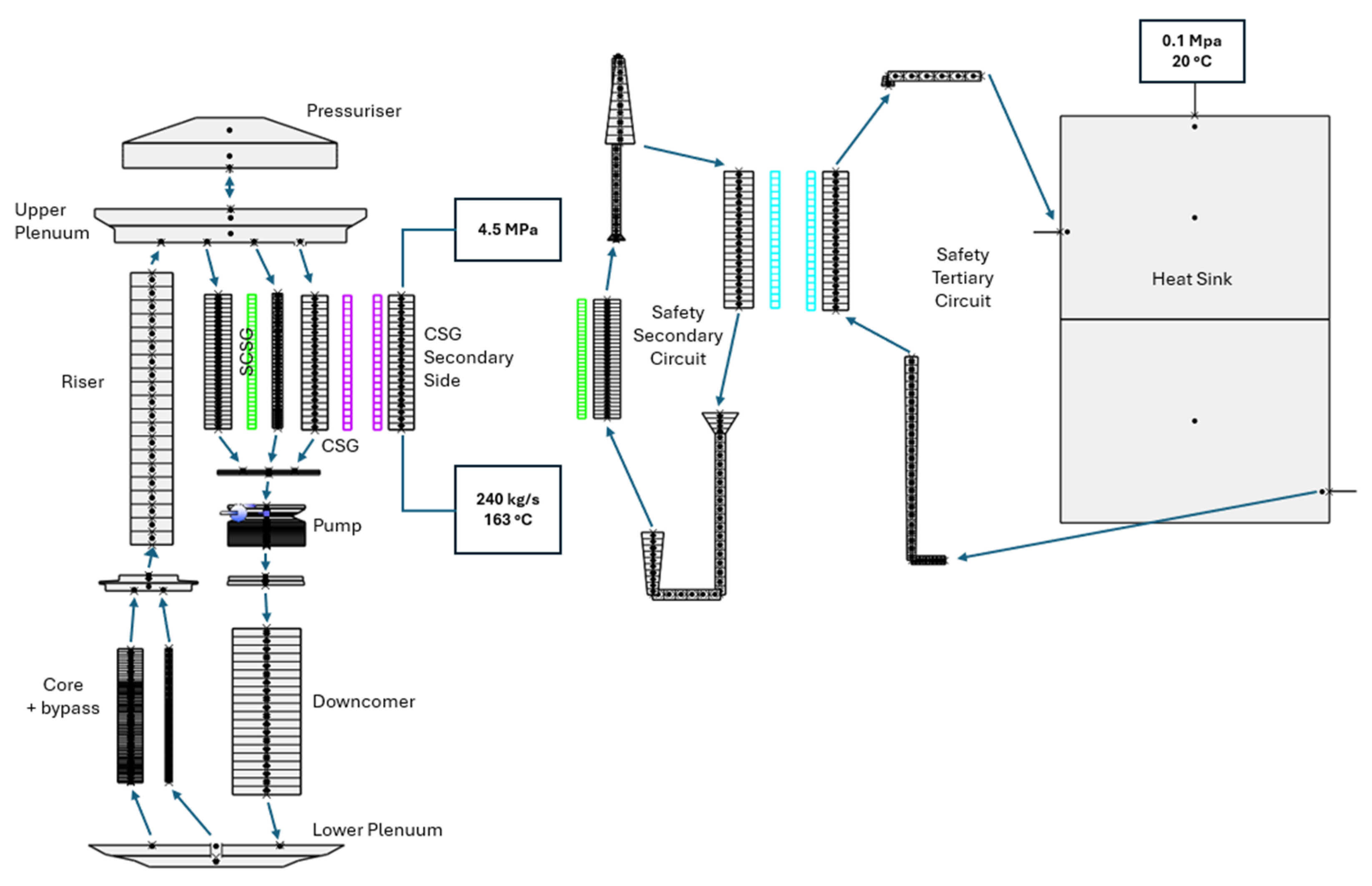
2.1. CATHARE 3 ESMR Model Description

The adopted ESMR model was developed with CATHARE 3 (v. 2.1), within the TANDEM project framework, based on an already available dataset (described in [29]) coming from a former European activity called ELSMOR. The ESMR conceptual design takes inspiration from the French integral LW SMR concept called NUWARD [30]. A detailed description of the ESMR model developed with CATHARE 3 can be found in the related public project deliverable [29]. In this paper, therefore, only the main characteristics of the ESMR are highlighted, referring the reader to the project deliverable for a more detailed description.

The ESMR is an integral type LW SMR composed of eight compact steam generators (CSG), six for normal operation conditions, and two conceived as safety features and named safety compact steam generators (SCGS). Each CSG is designed as a once-through plate heat exchanger with rectangular channels both for the primary and secondary side, used to produce superheated steam. The cooling of the core is made by forced circulation through six primary pumps, i.e., one per each CSG outlet. The SCSGs, instead, are designed to work under natural circulation to dissipate the decay heat from the core to a secondary safety circuit, also driven by natural circulation, which in turn exchanges heat with a tertiary circuit that discharges the accumulated thermal energy in a water pool that has the function of the ultimate heat sink. A layout of the primary circuit nodalisation developed with CATHARE 3 is shown in Figure 1, where the above-mentioned safety circuits are also represented together with the imposed nominal boundary conditions.

Table 1. Nominal conditions of the ESMR (source: [29]).

Parameter	Value
Primary Side
Core Thermal Power (MW)	540
Inlet Core Temperature (°C)	300
Core Coolant ΔT (°C)	24.5
Core Coolant Δp (MPa)	0.58
Pressuriser Pressure (MPa)	15
Coolant Mass Flow Rate (kg/s)	3700
Secondary Side
Feedwater Temperature (°C)	163
SH Steam Temperature (°C)	300
Outlet Pressure (MPa)	4.5
Coolant Mass Flow Rate (kg/s)	240

, instead, lists the main parameters of the ESMR during nominal conditions.

In the present model of the ESMR, the control systems described hereafter are implemented:

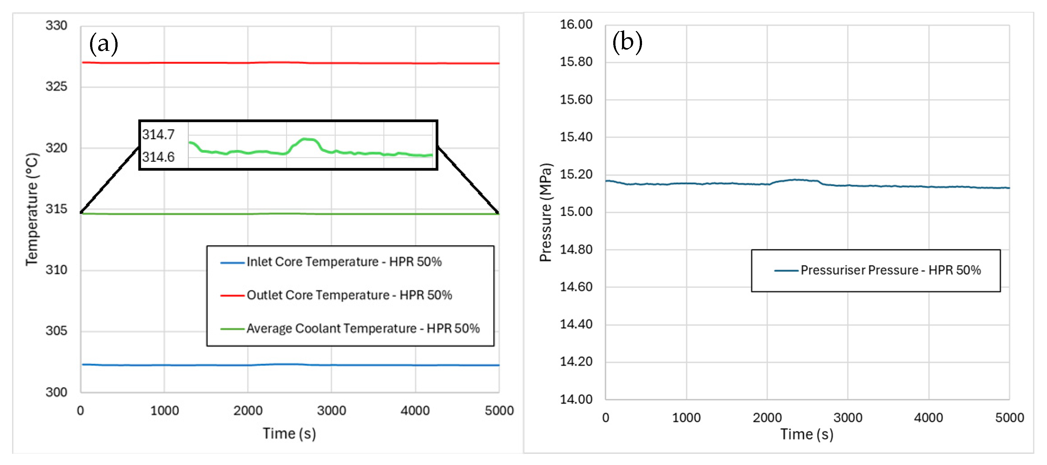
• Primary pressure control system, obtained through a spray valve and an electrical heater embedded in the pressuriser. The spray valve was modelled such that the enthalpy of the sprayed water is equal to the one achieved in the first node of the downcomer, where the feeding line is supposed to be connected, whereas the heater is considered simply as a point heat source.
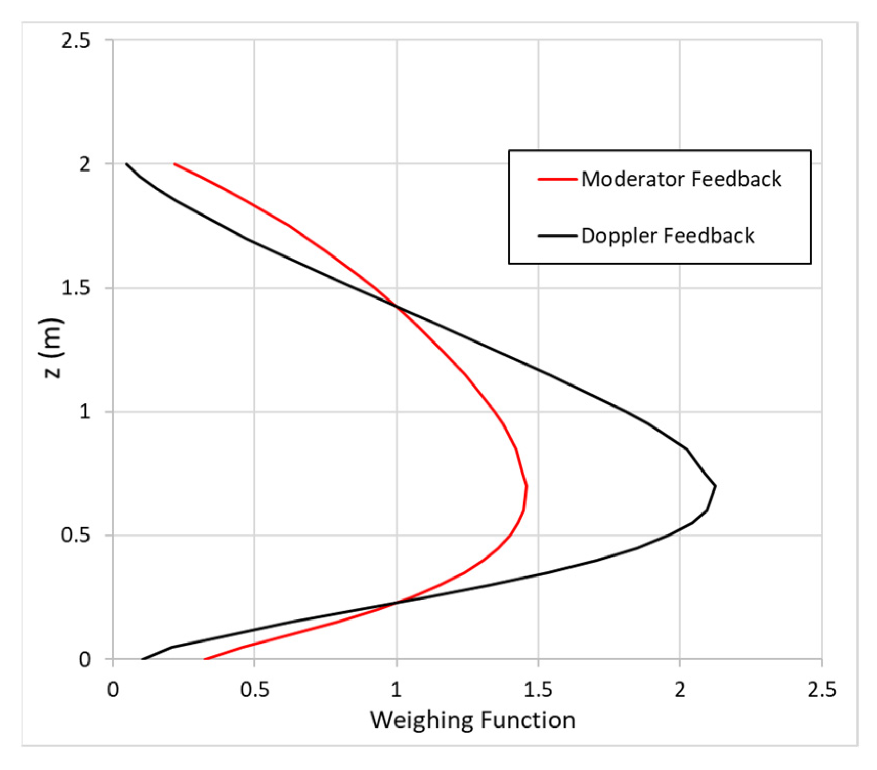
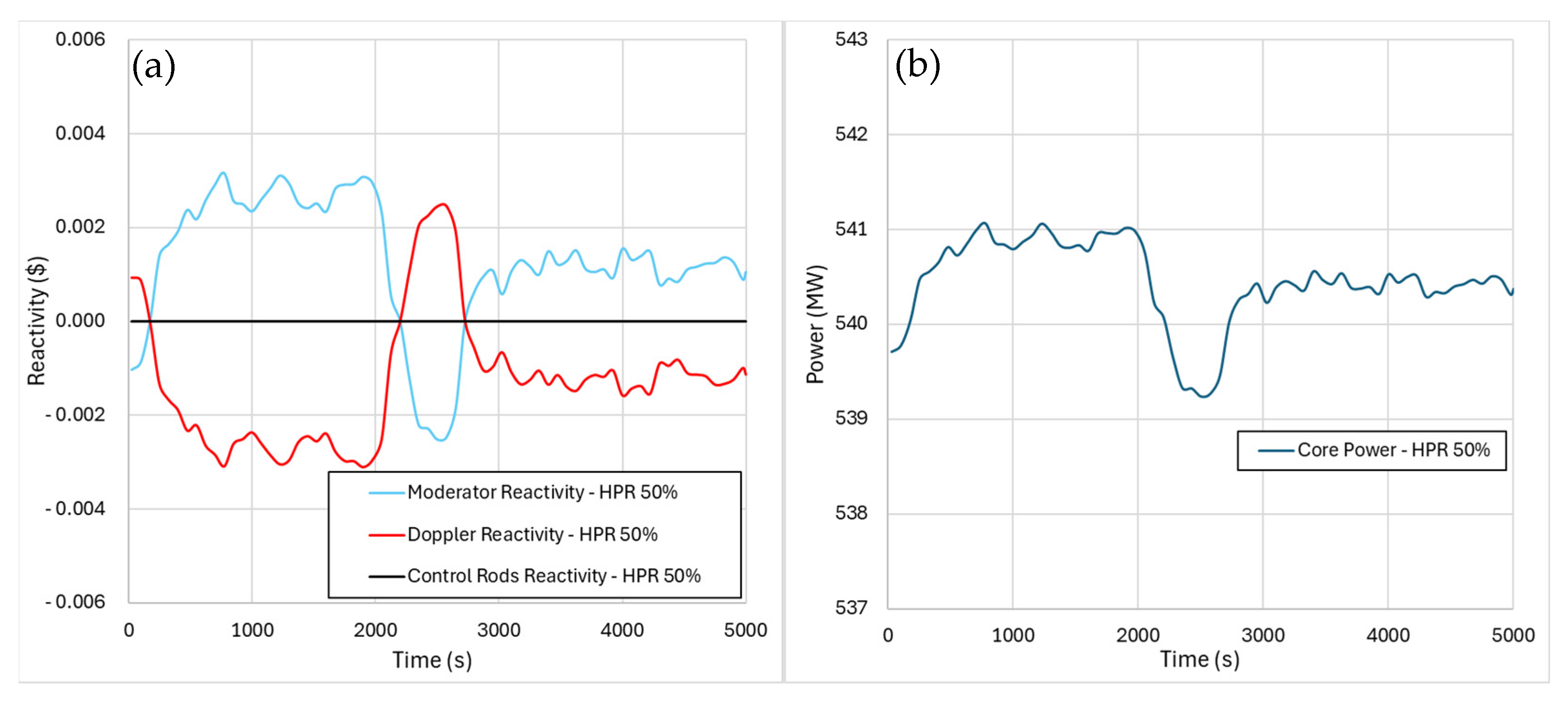
• Average core coolant temperature control system, implemented by means of control rods. The control rods were modelled as an external reactivity source, in line with the fact that CATHARE 3 solves a point core kinetic equation. Therefore, the details of the movement of the control rods and of their axial effects were neglected in the present model. In particular, the control rod reactivity insertion was implemented following a proportional–integral (PI) control function as the one reported in Equation (1), where $t^{\ast }$ is the time at which the control takes place and $k_P$ and $k_I$ are the proportional and integral gains, respectively.

$$r_{ext}(t)=k_{P}e(t)+k_I{\displaystyle \underset{t^{\ast }}{\overset{t}{\int }}e(t)dt}$$

(1)

In Equation (1), the error $e(t)$ is the deviation of the average core coolant temperature from its setpoint, as defined in Equation (2). Moreover, a dead band of ± 0.5 °C was imposed on the control rods, i.e., the control rods are activated only if $|e(t)|>0.5$ °C.

$$e(t)={\overline{T}}_{core}(t)-{\overline{T}}_{core,sp}$$

(2)

To consider the core neutronics, the delayed neutron precursors parameters listed in

Table 2. Neutronic parameters implemented in the ESMR CATHARE 3 model.

Group	${\mathit{\beta }}_{\mathit{i}}$ (-)	${\mathit{\lambda }}_{\mathit{i}}$ (s−1)
1	1.66·10−4	0.0125
2	1.02·10−3	0.0314
3	9.63·10−4	0.1102
4	2.72·10−3	0.3209
5	8.95·10−4	1.3280
6	2.89·10−4	3.01
TOT.	6.053·10−3	-

were introduced in the ESMR model. In this regard, it must be mentioned that the reference values of the delayed neutron fraction and decay constant of each precursor were taken as the ones implemented in the MODELICA model of the ESMR developed within the TANDEM project [25]. In fact, since the neutronic parameters introduced in the MODELICA library [26] are the result of a preliminary neutronics assessment carried out by the partners involved in the related modelling, they were considered as reference for the performed analyses.

In the adopted model, the radial power distribution in the core was assumed to be uniform (i.e., there is no distinction between hot and cold channels). However, the axial distribution of the power was imposed equal to the one of a generic Pressurised Water Reactor, coming by default with the CATHARE 3 code. The axial power distribution, moreover, was taken as reference to approximate the axial weighting of the contributions to the two reactivity feedbacks, i.e., Doppler and moderator density. In particular, the moderator reactivity feedback weighting was considered equal to the core power axial distribution, whereas the Doppler one was considered proportional to the square of the power, a result that comes from the perturbation theory applied to neutron diffusion problems (see, e.g., [31]). Figure 2 shows the trends of the weighting functions of the moderator and Doppler reactivity feedbacks.

It must be mentioned that the CATHARE solver performs the normalisation of the weighing functions during the calculation automatically. Boron reactivity effects were not considered, since the present design of SMR does not conceive it as part of the reactivity control of the coolant [25]. The total reactivity coefficients, instead, were considered equal to those already available in the CATHARE 3 code for a common PWR, which are 0.301·$/°C^1/2 and 6.62·10⁻² $·m³/kg for the Doppler and moderator feedbacks, respectively. In this regard, it must be mentioned that the adoption of core data coming from a common PWR was dictated by the fact that neutronic data specifically related to the ESMR design were still missing at the time the present work was being carried out.

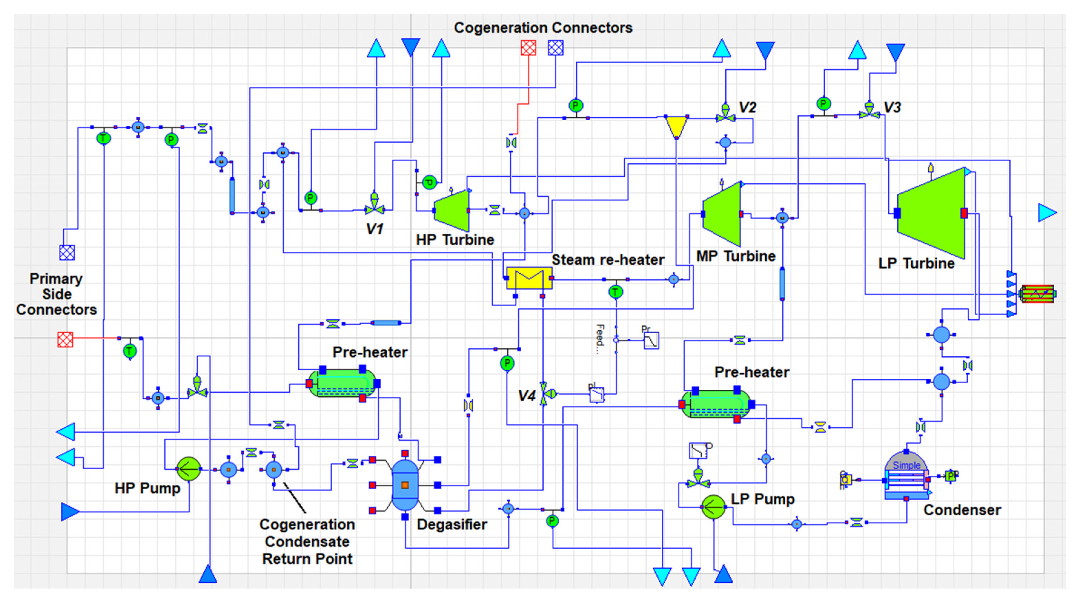
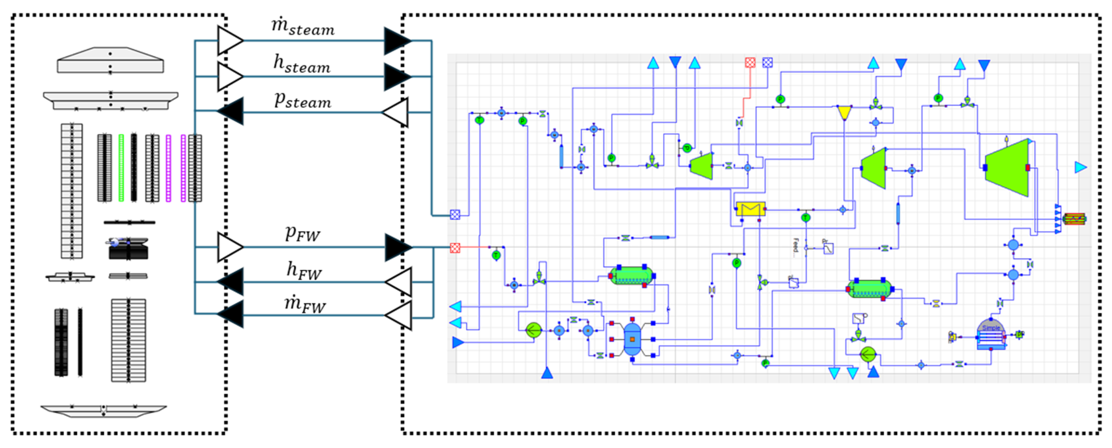
2.2. MODELICA BOP Model Description

The considered BOP model belongs to the TANDEM MODELICA library [25]. As indicated in Figure 3, it represents a quasi-static model of secondary system components belonging to the ThermoSysPro MODELICA library [32], which are only described by lumped parameter equations. The water thermophysical properties considered by the ThermoSysPro library are those belonging to the IAPWS-IF97 standard database [33]. The BOP modelling features are described in the related public project deliverable [25]. However, some of its main features are also described in this section for the sake of completeness. The present BOP model is very similar to a conventional steam cycle: it involves three steam turbines, i.e., high, medium, and low pressure, and a steam re-heater placed between the high and the medium pressure turbines. The steam turbines follow a Stodola ellipse law for the mass flow rate–pressure relation. After the low-pressure turbine, there is the condenser (that is the cold sink of this thermodynamic cycle) and two feedwater preheaters supplied by steam spilled from the turbines, modelled as lumped parameter heat exchangers (HX). A degasifier is introduced between the two feedwater pre-heaters, here considered as a simple volume tank. Two centrifugal pumps are considered, i.e., the condensate extraction pump, placed just after the condenser, and the high-pressure pump, which pressurises the feedwater to be injected into the steam generators. In Figure 3, the BOP layout is shown, where the connectors used to couple the BOP with the secondary side of the steam generator, modelled by CATHARE 3, are also highlighted; they will be used in translating the BOP model into FMU by means of related input/output ports also belonging to the ThermoSysPro MODELICA library [32].

The only difference this model has with respect to a conventional BOP for electricity production is the steam bypass line placed after the high-pressure turbine, which allows the extraction of steam, to be sent into another block, modelling the cogeneration sector of the BOP. The coupling between BOP and the cogeneration section is made through related connectors, also highlighted in Figure 3. The extracted steam, once condensed, is again introduced in the steam cycle in saturated liquid state in a control volume placed just before the HP pump, as indicated in Figure 3. The cogeneration sector, shown in Figure 4, contains a heat exchanger, which takes the place of the heat exchanger used to supply thermal power to a heat user coupled with the nuclear power plant. The cogeneration HX is an ideal condenser, i.e., the outlet flow is always considered at saturated liquid state no matter the inlet conditions. The steam mass flow rate extracted from the BOP is controlled by the cogeneration control valve (CCV) shown in Figure 4, which is governed by a proportional–integral (PI) controller. In fact, the CCV controller aims to make the thermal power exchanged by the cogeneration HX follow the one imposed as a boundary condition, i.e., the thermal load demand of the heat user.

In the present BOP model, other PI control systems were introduced, including the following:

• Main steam line control system: PI controller which commands the high-pressure turbine inlet valve (indicated with V1 in Figure 3) to maintain the main steam line pressure at its setpoint value.
• Medium and low-pressure turbine inlet pressure control system: PI controllers that command the opening of valves V2 and V3 to control the pressure at the inlet of the medium- and low-pressure steam turbines, respectively.
• Re-heater steam mass flow rate controller: PI controller which controls the steam temperature at the outlet of the re-heater (i.e., inlet of medium pressure turbine) acting on the valve V4.
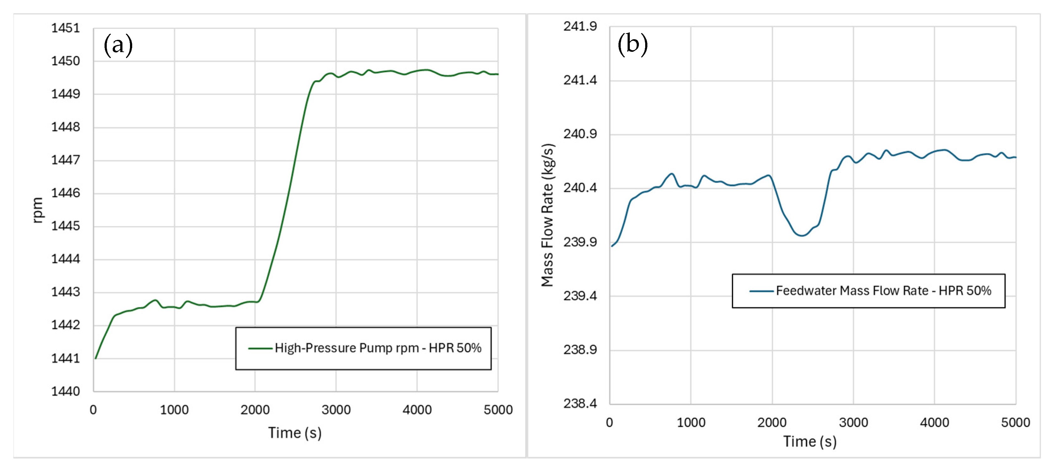
• High-pressure pump rotational speed controller: PI controller which varies the rotational speed of the high-pressure pump (i.e., the feedwater mass flow rate entering the CSG) to keep the steam temperature constant.
• Low-pressure pump rotational speed controller: PI controller which controls the water pressure at the inlet of the degasifier by varying the rotational speed of the low-pressure pump.

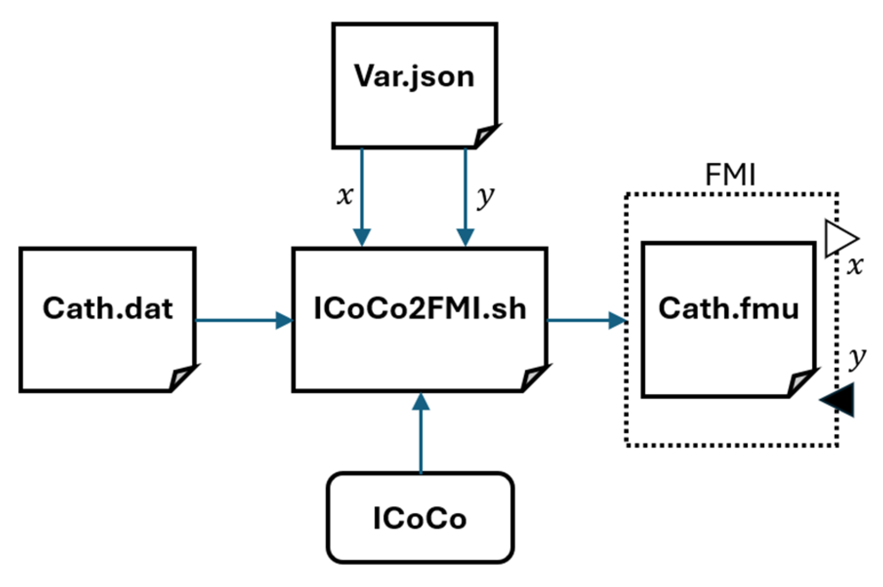
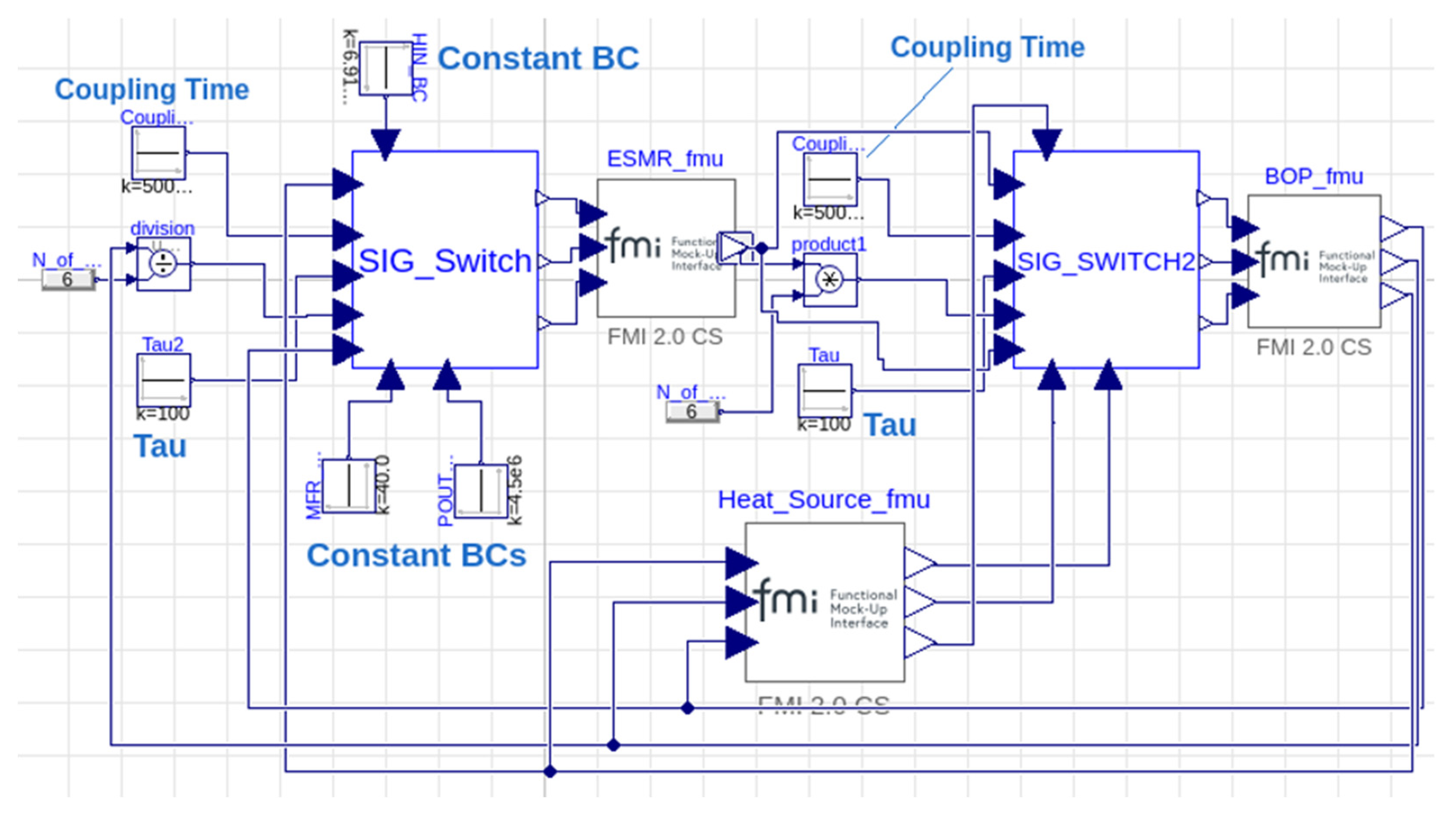
3. Description of the Coupling Strategy

The coupling between the two considered codes, i.e., CATHARE 3 and MODELICA, was performed by adopting the Functional Mock-up Interface (FMI) tool [23]. In this case, FMIs for co-simulation are used, i.e., the FMIs embed the solver within the model [23]. In order to allow for the coupling between two models through FMI, their translation into Functional Mock-up Units (FMU) is necessary. In this regard, it must be mentioned that the BOP FMU was generated by embedding the CVODE, available in the package, as the reference solver.

The MODELICA model of BOP, described in the previous section, was translated into FMU by using Dymola 24x [24], a commercial environment used to run simulations with MODELICA models. For the CATHARE 3 model, instead, a different procedure was adopted to perform its translation into FMU, which involved the adoption of a C++ classes library, namely Interface for Codes Coupling (ICoCo) [34], and an executable shell file called ICoCo2FMI [35]. Moreover, a JSON (JavaScript Object Notation) file is needed to define the variables to be extracted by the CATHARE 3 model and be set as input/output on the generated FMI for the coupling. By running ICoCo2FMI using ICoCo as reference library for the translation, therefore, the CATHARE 3 model is translated into FMU and the related FMI is built, having as input and output variables those indicated in the above-mentioned JSON file. The translation procedure is explained in greater detail in a previous work [22]; however, Figure 5 summarises in a sketch the procedure used for the CATHARE 3 model translation. It must be mentioned that the present translation procedure only works with CATHARE 3 v3.1 or more recent versions of the code.

Following the rationale adopted for the modelling of the primary and secondary loops, a fluid coupling is selected for this application as a novel choice, meaning that the two models of primary and secondary side are made to exchange fluid boundary conditions during the co-simulation, instead of a mere heat transfer power. In fact, given that the entire CSG is modelled by CATHARE 3, including primary and secondary fluids (see again Figure 1), the imposed boundary conditions (i.e., feedwater mass flow rate, feedwater enthalpy, and steam pressure) are adopted to couple it with the BOP model, thus receiving and injecting the calculated fluid flows. With this choice, the ESMR imposes to the BOP fluid boundary conditions, calculated based on its internally computed variables, in terms of steam mass flow rate and enthalpy and feedwater pressure, thus achieving a numerical coupling such as the one illustrated in Figure 6.

To supervise the co-simulation, Dymola 24x was used, adopting the implicit DASSL algorithm [36]. The adopted strategy to perform the coupling adhered to the inherent numerical structure of the CATHARE 3 code, which requires a first steady-state calculation and then a stabilised transient analysis before being ready to start the simulation of the addressed transient scenario [37]. During the first iterations of the BOP model, simultaneous with the stabilised transient performed by the CATHARE 3 solver, the behaviour of the two models may show excursions due to the unavoidable unbalances in the initial conditions and to the need to stabilise the solution evaluated by the different numerical algorithms. Given this, coupling the two models after an appropriate delay is suggested, waiting for stabilisation of the independent behaviours after the end of the CATHARE 3 stabilised transient.

Therefore, a specific switching logic was developed for gradually changing the boundary conditions during the coupling, using blocks belonging to the MODELICA Standard Library [27], which adopt a smoothing function $\psi (t,\mathit{\tau })$, reported in Equation (3), based on useful properties of the hyperbolic tangent:

$$\psi (t,\mathit{\tau })={\displaystyle \frac{1}{2}}\left[1-\tanh \left({\displaystyle \frac{t-\tilde{t}}{\mathit{\tau }}}\right)\right]$$

(3)

In Equation (3), $\tilde{t}$ indicates the time when the coupling occurs and $\mathit{\tau }$ is a time constant determining the reference relaxation time needed to perform the complete switch between two different boundary conditions. Therefore, the developed block performs the switch between two signals, namely $x_1(t)$ and $x_2(t)$, so that the output signal $y(t)$ results as in Equation (4):

$$y(t)=\psi (t,\mathit{\tau })x_1(t)+\left[1-\psi (t,\mathit{\tau })\right]x_2(t)$$

(4)

This apparently second-order detail turned out to be quite necessary to avoid to negatively influencing the dynamics of the ongoing coupling by changes in boundary conditions that were too sudden.

In the present case, the parallel stand-alone run of the two models is performed by imposing constant boundary conditions on the ESMR, equal to the nominal ones, and by coupling the BOP model with a lumped parameter heat source, also belonging to the TANDEM MODELICA library [26]. The 0D heat source, which substitutes the nuclear steam supply systems (NSSS), is generally used to carry out tests on BOP models without the need to consider the entire model of the primary side. Figure 7 shows the layout of the coupling block, where the switches, namely SIG_SWITCH and SIG_SWITCH2, are shown together with the three involved models (i.e., ESMR, BOP, and 0D heat source).

It can be noticed in Figure 7 that the two switches were developed such that the two parameters required by them, i.e., the coupling time $\tilde{t}$ and the time constant $\mathit{\tau }$, are externally provided, thus introducing flexibility in performing their tuning process. In the present analyses, the time constant $\mathit{\tau }$ was set equal to 100 s and the coupling time $\tilde{t}$ equal to 5000 s, as is better explained in the next section.

4. Description of the Addressed Transient Scenarios

One of the activities of the TANDEM project concerned a literature review about safety aspects of nuclear cogeneration (see, e.g., [16,38]). In this work, several references were considered coming from different European research activities and reports from international agencies and research organisations. All the considered works agree on the fact that the envisaged heat user, coupled with the nuclear power plant, must not decrease its general level of safety. For this reason, the code coupling was adopted to assess different transients which are foreseen to be induced by the heat user on the BOP and, consequently, on the primary system.

In general, all the analyses carried out in the present work were preceded by a 5000 s of stand-alone and separated run of the two models, as described in the previous section. Since the core neutronic model is activated only at the end of the CATHARE 3 stabilised transient, the 5000 s of independent run covered 2500 s of the stabilised transient and another 2500 s after the core neutronic activation to stabilise its parameters before the coupling. Therefore, all the trends presented hereafter refer to the time after coupling, i.e., to the physical time starting after the coupling occurrence.

Following this rationale, different transients were considered belonging to normal operation (NO) conditions or anticipated operational occurrences (AOO), depending on whether the transient is planned ahead or not [39]. In fact, the present analyses only focused on NO without considering Design Basis Accident (DBA) conditions, which normally bring about a physical separation between the primary and secondary systems [39]. The addressed scenarios are described hereafter.

4.1. Cogeneration Start Transients

During these analyses, a change in the thermal load required by the heat user is considered, starting from a nominal full-electric operation of the nuclear power plant. As mentioned in the previous paragraph, this type of transient can be considered as a NO condition, if the operation change is planned, or as AOO if unplanned [39]. Therefore, the main goal of these analyses is to understand what the response of the nuclear reactor to a change in the behaviour in the BOP could be, switching from full-electric to cogeneration operations. To assess these scenarios, values of thermal power related to different heat-to-power ratios (HPR) were considered, i.e., from 10% to 50%. For the sake of clarity, the heat-to-power ratio is here defined as in Equation (5):

$$HPR={\displaystyle \frac{{\dot{Q}}_{cog}}{{\dot{W}}_{el,nom}}}$$

(5)

where the cogeneration thermal power ${\dot{Q}}_{cog}$ is simply evaluated by a thermal balance performed on the cogeneration HX, being the enthalpy difference known due to the simplifying assumptions adopted for its modelling described in the previous section.

Therefore, considering that in nominal full-electric conditions, the modelled nuclear power plant produces 173 MW of electricity [25], the values listed in

Table 3. Nominal thermal demand of the heat user for different heat-to-power ratios.

HPR	Heat User Thermal Power Demand (MW)
10%	17.3
20%	34.6
30%	51.9
40%	69.1
50%	86.5

were used as boundary conditions to assess the cogeneration transients.

The thermal demand was imposed through a ramp which lasted 10 min (i.e., 600 s), starting from 2000 s of time after coupling, as shown in Figure 8. During the present analyses, no external action was envisaged for the nuclear power plant, i.e., the system was left spontaneously evolving in response to the transient thanks to the control systems implemented in both the primary and secondary side, as described in previous sections.

4.2. Core Power Variations During Cogeneration

During these analyses, a decrease in the core power during a cogeneration operation of the nuclear power plant was assessed, with the main objective of understanding whether a decrease in the core power caused by, e.g., a decrease in the electrical demand, would influence the capability of the BOP of providing the required thermal power to the heat user. In this regard, it must be highlighted that the adopted model of BOP does not provide a model of the electrical load. Indeed, in nuclear power plants, if a change in the electrical power demand occurs, the mechanical power of the turbines follows the change in the electrical one to assure the equality between the mechanical and electrical torques. This leads to a shift in the operational conditions of the BOP, which in turn affects the core power through the reactivity feedbacks and, in that case, to the triggering of the insertion/extraction of some banks of control rods specifically used for load following (grey control rods) [40]. In this case, however, since the electrical load is not considered and the model is quasi-static, it is assumed that the nuclear power plant operates in an infinite grid which does not respond to any change in the generated electrical power.

Therefore, in the present case, the core power was decreased by simulating the insertion of the control rods through a specific control function making use of the core power $\dot{Q}$, as in Equation (6), thus inserting negative external reactivity to bring the reactor thermal power to the required setpoint value, ${\dot{Q}}_{SP}$:

$$r_{ext}=k{\displaystyle \underset{t^{\ast }}{\overset{t}{\int }}\left({\dot{Q}}_{SP}-\dot{Q}\right)}dt$$

(6)

In this analysis, starting from nominal full-electric operation of the coupled system, a cogeneration transient was first induced, starting at 2000 s, such as the ones shown in Figure 8 with HPR 50%. Then, at 4000 s of physical time, the core power was decreased by up to four different values, from 90% to 60% of the nominal one of 540 MW.

4.3. Thermal Load Rejection

The last analysis aimed to assess the capability of the coupled system in dealing with an AOO, which was considered to be caused by the loss of the cogeneration load. In this regard, the adopted boundary condition for the cogeneration thermal power is shown in Figure 9.

As it can be noted in Figure 9, starting from operation in full-electric conditions, first an increase in cogeneration was assumed, reaching 50% of heat-to-power ratio with a ramp starting at 2000 s and lasting 600 s. After 1000 s of operation in these conditions, the thermal demand suddenly dropped to 0 MW. This may simulate a failure in the heat user or in the thermal circuit connecting it with the nuclear power plant. This event was called “thermal load rejection” in similarity to a load rejection involving the electrical load. As for the cogeneration transients, also in this case no external action was conceived after the occurrence of the AOO event, i.e., the coupled system was left evolving spontaneously up to 8000 s thanks to the implemented control systems on both the primary and secondary sides of the plant.

5. Obtained Results

Before the discussion of the obtained results, some considerations must be introduced to clarify some of the technicalities that made it possible to obtain them. In all the analysed cases, after the occurrence of coupling, the system was left stabilising for 2000 s before starting the transient. The new stationary condition achieved with the coupled system was generally found to be slightly different from the one achieved by each model while running independently. Such deviations are mostly related to the inherent differences in the two modelling tools, i.e., CATHARE 3 and MODELICA, in evaluating relevant parameters which are then provided as boundary conditions to either module after coupling. Though these deviations cannot be completely avoided due to the inherent differences in the models of the two codes, the imposed boundary conditions for the independent run of the two models could be tuned to bring them to more coherent stand-alone stationary conditions. Noticeably, some small oscillations were achieved during the coupled analysis, likely related to small instabilities occurring during the coupling, which may be considered a matter for further improvement in future applications.

As already mentioned, the BOP model adopted in the present analyses is quasi-static, i.e., the component dynamics are neglected. This simplifying hypothesis certainly affects the behaviour obtained for the relevant parameters in response to the different addressed transient scenarios. Also, the adopted control strategy was dependent on the particular simplifying assumptions adopted during the modelling of the two systems, i.e., ESMR and BOP. Indeed, the adoption of different control strategies, e.g., those normally adopted for a dynamic BOP, may have led to different behaviours of the systems during the addressed scenarios, which is something that must be taken into consideration while describing the results coming from the present analyses.

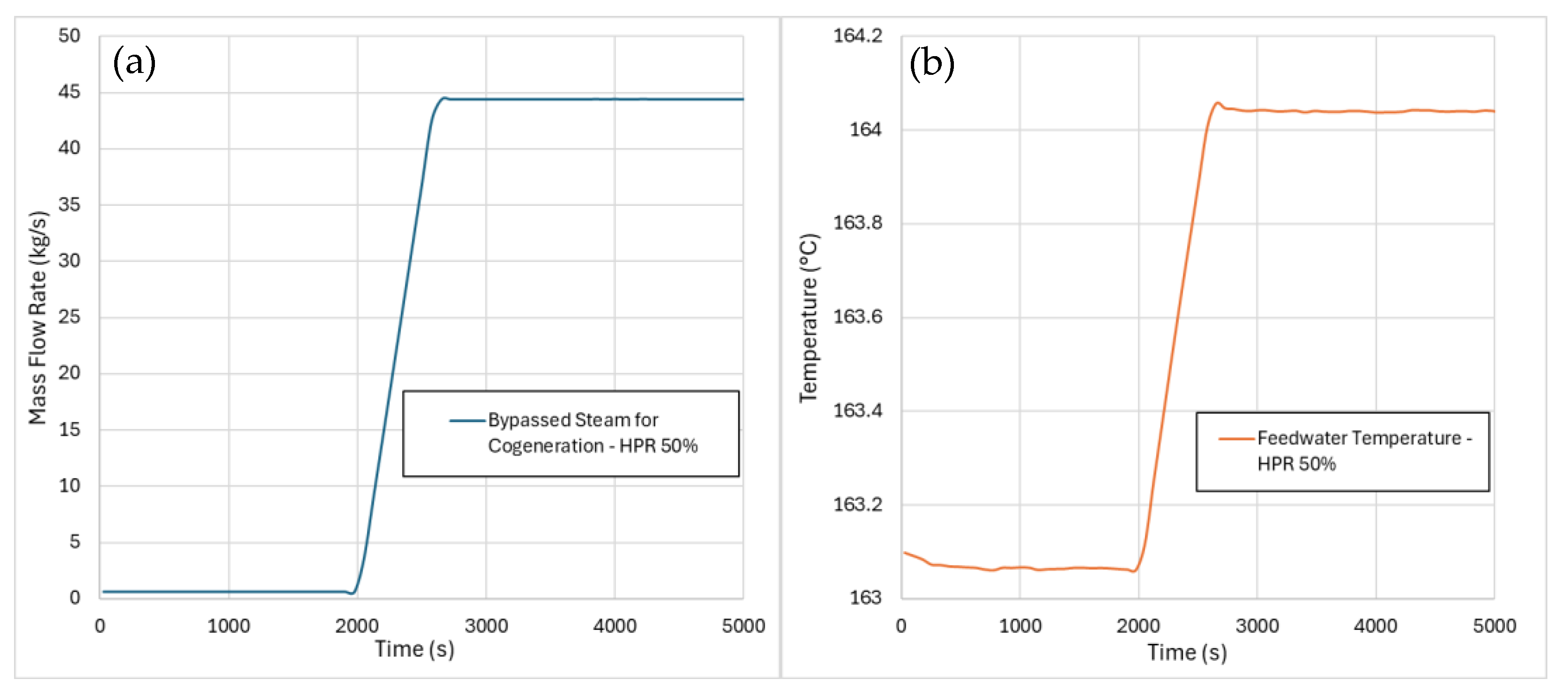
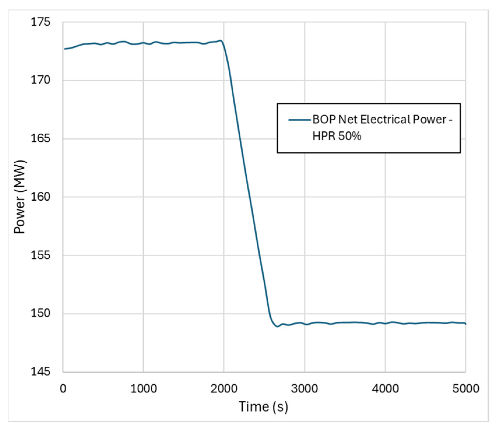
5.1. Results from Cogeneration Start Transients

Though the analyses have been performed for all the cases shown in Figure 8, only the case with highest heat-to-power ratio (i.e., 50%) is considered here, being the most meaningful in terms of primary side response; the results of the other analyses are qualitatively similar to the ones presented here. As shown in Figure 10a, the increasing thermal power demand required by the heat user shown in Figure 8 leads to the opening of the cogeneration control valve and hence to the bypass of a certain amount of steam from the BOP to the cogeneration heat exchanger. Consequently, hot condensate was reinjected in the feedwater line shown in Figure 3; the merging of the two flows, i.e., feedwater and hot condensate, led to the increase in the feedwater temperature entering the steam generator, as shown in Figure 10b. The increase in the feedwater temperature tended to also increase the steam temperature exiting the steam generator, which triggered the high-pressure pump controller, thus increasing the pump rotational speed as depicted in Figure 11a. Moreover, the increase in the feedwater temperature also led to the temporary decrease in its mass flow rate, as shown in Figure 11b, caused by the lower density of the feedwater and by the increased void fraction in the CSG. Then, the feedwater mass flow rate was recovered in the last part of the transient, thanks to the stabilisation of the feedwater temperature and to the higher rotational speed of the secondary pump. The superposition of the lower mass flow rate and of the higher temperature of the feedwater decreased the thermal power exchanged with the CSG, thus leading to a heating up of the primary coolant. The increase in the primary temperature and pressure, however, ended up being very mild, as illustrated in Figure 12a,b. Therefore, both the primary pressure and average temperature were found to be almost not influenced by the transient, being the total deviation of the average core coolant temperature lower than 0.1 °C.

Nevertheless, the slight increase in the primary coolant temperature was sufficient to trigger a visible change in the neutronic feedbacks, resulting in a decrease in the core power, as can be seen in Figure 13a,b. It is interesting to notice that the control rods did not enter into operation due to the average core coolant temperature’s small deviation, shown in Figure 11a, which remained within the adopted dead band of ±0.5 °C.

Figure 13a also shows that the reactivity feedbacks stabilised at a value different than 0, being the level obtained by the separated calculations, during the full-electric state of the coupled system, owing to the deviations that occurred after the coupling with respect to those achieved during the independent runs. Moreover, from Figure 13a, it is also clear that a very slight instability is also obtained after the transient occurrence. As explained in the previous sections, these slight imbalances may be caused by the inherent differences in the two models or, at the same time, by numerical disturbances brought about by both solvers (i.e., those of the two FMU) which may have been amplified, although not in a divergent way, by the coupling. As mentioned before, during the start of the cogeneration transition, the primary coolant was slightly heated up, thus leading to an insertion of negative reactivity due to the moderator feedback. In response to the core power decrease, the Doppler effect inserted a corresponding positive reactivity, almost balancing the moderator neutronic feedback and resulting in a very small shift in the overall reactivity. In addition, Figure 13a shows how the core power stabilised at a lower value after the cogeneration transition occurrence with respect to full-electric operations, considered equal to 540.89 MW, evaluated as the average value between 1000 s and 2000 s. In this regard, the new thermal power of the reactor was found to be equal to 540.39 MW during the cogeneration, again evaluated as an average between 3000 and 5000 s. The lowest peak achieved by the thermal power of the reactor was 539.23 MW, which is 0.3% lower than the value of the full-electric case, further proving the mild influence the cogeneration transient had on the primary circuit. As expected, the net electrical power produced by the BOP was instead considerably decreased by the activation of the cogeneration as shown in Figure 14, mainly due to the lower mass flow rate flowing through the lower pressure stages of the steam turbines.

To conclude this description,

Table 4. Results from cogeneration transients.

HPR	Nominal Core Power (MW)	Thermal Power Delivered to the Heat User (MW)	Core Power with Cogeneration at Steady State  ${\dot{\mathit{Q}}}_{\mathit{c}\mathit{o}\mathit{r}\mathit{e}}$  (MW)	Net BOP Electrical Power  ${\dot{\mathit{W}}}_{\mathit{e}\mathit{l},\mathit{n}\mathit{e}\mathit{t}}$  (MW)	Combined System Efficiency (%)
0%	540.89	-	-	173.30	32.0
10%	540.89	17.30	540.66	168.50	34.3
20%	540.89	34.60	540.62	163.60	36.6
30%	540.89	51.90	540.55	158.60	38.9
40%	540.89	69.10	540.50	153.80	41.2
50%	540.89	86.50	540.39	149.20	43.6

lists some of the main results obtained from the five analyses carried out in comparison with a full-electric case, also showing how the cogeneration increased the global energy efficiency, as reported in Equation (7), which attributes the same value to the electrical and thermal energy, of the considered steam cycle.

$$\eta ={\displaystyle \frac{{\dot{W}}_{el,net}+\left|{\dot{Q}}_{cog}\right|}{{\dot{Q}}_{core}}}$$

(7)

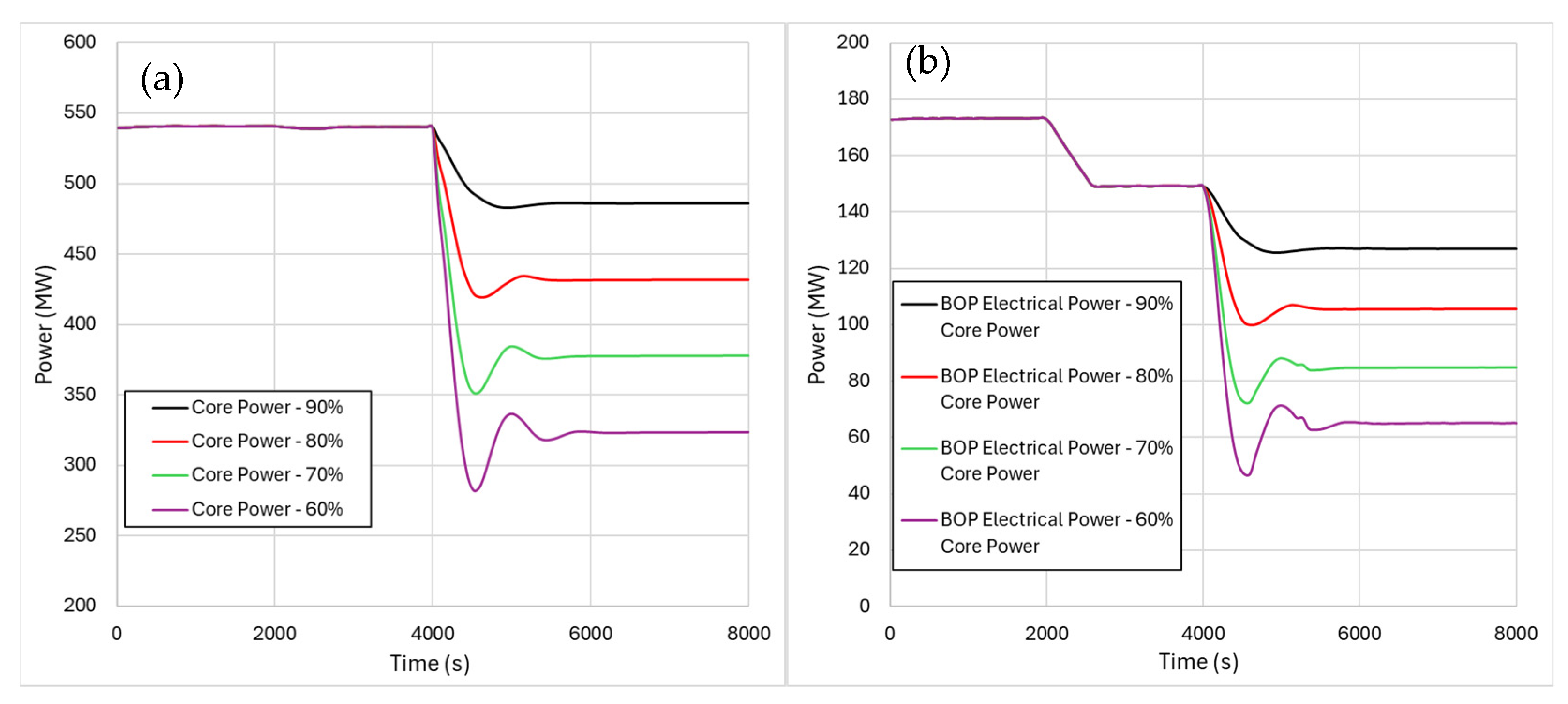
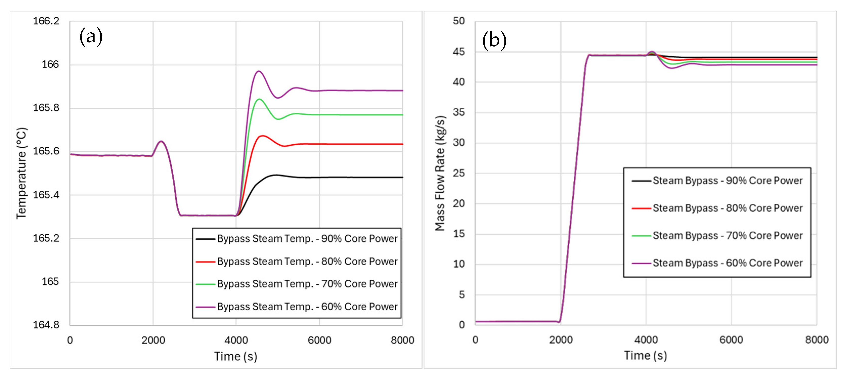
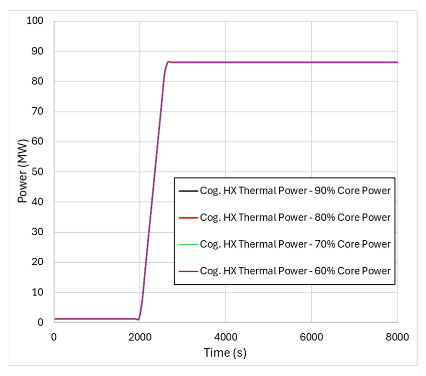
5.2. Results from Core Power Variation Transients

After a cogeneration transient with HPR 50%, the core power was decreased to four different values, as shown in Figure 15a. As can be noted, the core power experienced some slight oscillations in the cases of highest decreases, due to the integral control function, adopted to simulate the insertion of the control rods and defined in Equation (6). These oscillations were also tolerated as a mean to better test the stability of the coupling and their presence was considered acceptable for the present analyses. The decrease in the core power immediately led to the decrease in the primary coolant pressure and temperature, resulting in a consequent decrease in the steam temperature exiting the steam generator, as shown in Figure 16a. Then, as is depicted in Figure 15b, the controller of the secondary pump decreased the mass flow rate to keep the steam temperature at its setpoint. The lower secondary mass flow rate led, therefore, to the decrease in the electrical power produced by the BOP, as shown in Figure 16b, where a decrease in the produced electricity can be noted due to the cogeneration at 2000 s and, subsequently, to the decrease in the core power.

The reduced secondary mass flow rate also led to a higher enthalpy at the output of the high-pressure steam turbine. For this reason, the bypass steam flow rate supplying the cogeneration heat exchanger was found to slightly decrease with the decrease in the core power, as shown in Figure 17a,b. Besides these deviations, however, it is interesting to notice how the system actually allowed the supply of constant thermal power to the heat user, notwithstanding the lower power production in the reactor core, as shown in Figure 18.

5.3. Results from Thermal Load Rejection Transients

The thermal load rejection event occurring at 3600 s triggered the instantaneous closure of the cogeneration control valve, leading to a sharp increase in the electrical power produced by the BOP, as shown in Figure 19, and, at the same time, to a sharp decrease in the feedwater temperature entering the steam generator (see Figure 20a).

As a result, the feedwater mass flow rate experienced the sharp rising peak depicted in Figure 20b, followed by a fast recovery back to the nominal value of the full-electric case.

Following the rapid increase in the secondary mass flow rate, the thermal power requested by the steam generator increased in consequence and the primary coolant temperature decreased as shown in Figure 21. The very sharp decrease in the average core coolant temperature soon triggered the moderator neutronic feedbacks, which inserted a peak of positive reactivity into the core, as shown in Figure 22a. Simultaneously, the Doppler effect reacted by introducing negative reactivity into the core due to the rapid heating-up of the fuel. The superposition of the two feedbacks brought the core power to a maximum peak of 545.38 MW, as shown in Figure 22b, which is almost 1% higher than the core power reference value of 540.39 MW achieved during a stationary cogeneration operation with HPR 50% (see again Table 4). It is interesting to notice that, like the cogeneration transients, the control rods did not enter into operation since the average core coolant temperature deviation was kept within the dead band of ±0.5 °C.

To conclude this section, it is important to remember that, as for the other presented cases, here, the quasi-static nature of the BOP model could have sensibly affected the results. In fact, the sharp change in the adopted boundary conditions shown in Figure 9 instantaneously affected the output parameters (i.e., feedwater temperature) and, in turn, the primary system. Therefore, the introduction of delays due to the component dynamics and the adoption of a different control strategy may bring about slightly different behaviour of the primary system compared to the addressed AOO event. In particular, the sharp variations obtained in these analyses could also be more limited in presence of component dynamics.

However, as one of the most important objectives of this work, the developed code-coupling methodology proved to be robust enough in dealing with such sharp changes in the operating conditions of the system. This can be considered as proof of the potential of the adopted methodology in assessing nuclear cogeneration transients, also using models with different complexity.

6. Conclusions

In this paper, the influence that meaningful cogeneration transients may have on the primary system of a nuclear LW SMR plant was assessed. The analyses were carried out using a novel approach based on fluid coupling achieved between models developed with two different tools, i.e., the thermal hydraulic system code CATHARE 3 and the dynamic modelling language MODELICA. Both the CATHARE 3 model of the reference LW SMR and the quasi-static BOP model are a product of a European research activity, performed in the frame of the TANDEM project. Simplifying assumptions were adopted in the modelling strategy in the present phase of analysis, mostly linked to the inherent structure of the adopted codes and to the preliminary character of this assessment, mostly concentrated on the coupling methodology. Each model was equipped with control systems to allow them to cope with the addressed transient scenarios. The resulting co-simulation was supervised using Dymola 24x, with the implicit DASSL algorithm.

During the present analyses, three meaningful transient scenarios that a heat user may induce in the nuclear power plant were considered, namely cogeneration start transients, core power variation transients, and thermal load rejection. In the limit of the adopted simplifying assumptions, the obtained results provide sufficient insight into the predicted response of a nuclear system to NO or AOO transients induced by the cogeneration. In particular, the following paragraphs summarise the obtained results:

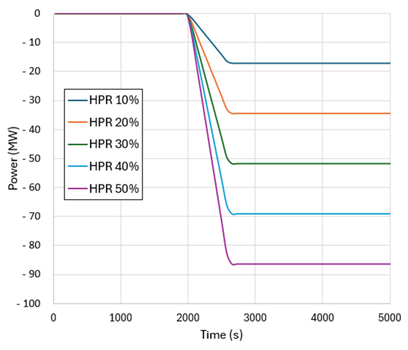
• The cogeneration start transients show that the primary system was mildly influenced by a switch from full-electric to cogeneration operation, with different values of the heat-to-power ratio. In this regard, the highest value of HPR led to a negative core power excursion of 0.3% with respect to the reference nominal value. Moreover, as expected, the cogeneration resulted in an increase in the overall energy efficiency of the steam cycle, as a specific objective of its adoption.
• The core power variation transient results highlight the capability of the modelled nuclear power plant in handling core power variations while performing cogeneration. As a matter of fact, the BOP, thanks to the implemented control systems, was found to be capable of handling core power decreases of up to 60% of the nominal value, while keeping the thermal power provided to the heat user unchanged.
• The thermal load rejection scenario may be the case where the quasi-static assumption of the BOP may have mostly influenced the results, since the sharp change in the boundary conditions was instantaneously reflected on the output parameters and, in turn, on the primary side. However, the results further prove the stability of the developed code-coupling methodology and, in addition, they also show that the primary system was capable of handling such transient only relying on the modelled neutronic feedback.

Therefore, the achieved results show that no sensible impacts are predicted on the primary side following the addressed transient scenarios, considering a range of thermal power diverted for cogeneration applications within 15% of the core rated value. However, the influence of the presently adopted simplifying assumptions must be carefully addressed by means of quantitative analyses. Moreover, the root causes of the small oscillations obtained during the numerical coupling, although they did not influence the general stability of the calculations, must also be investigated. In addition, the reliability of the results coming from the adopted coupling methodology must be further assessed using available data coming from experimental campaigns or real-world operations. However, being Hybrid Energy Systems still in the conceptual design phase, neither operational data or real-world prototypical applications are present yet. However, future works may concern code-to-code comparison between the numerical coupling and other well assessed numerical codes in order to obtain a more comprehensive overview of the qualitative reliability of the developed coupling tool.

The analyses carried out and the developed methodology are open to a wide range of possible further applications, e.g., making use of more sophisticated models of both primary and secondary side. The developed coupling strategy has the advantage of relying on unified tools, i.e., FMIs, leading to the possibility of planning analyses with a much more detailed model of the heat user and of the intermediate thermal circuit connecting the nuclear power plant to it and of other involved components, such as the electrical grid, achieving a more comprehensive tool capable of providing more detailed information about nuclear cogeneration safety. Moreover, when additional details of the presently adopted SMR design become available, more sophisticated models of the primary circuit can be considered, leading to more quantitatively meaningful analyses. The adopted methodology can also help to perform comprehensive Probabilistic Safety Assessment studies, which will be necessary to assist in the development and safety assessment of hybrid systems of nuclear power plants which are needed to meet the required decarbonisation goals of the future world energy mix.

References

1. International Panel on Climate Change. Climate Change 2023 Synthesis Report, Contribution of Working Groups I, II and III to the Sixth Assessment Report of the Intergovernmental Panel on Climate Change; Core Writing Team, Lee, H., Romero, J., Eds.; IPCC: Geneva, Switzerland, 2023; pp. 35–115. [Google Scholar] [CrossRef]
2. United Nations. Paris Agreement. 2015. Available online: https://unfccc.int/sites/default/files/english_paris_agreement.pdf (accessed on 4 April 2025).
3. International Energy Agency. Net Zero by 2050: A Roadmap for the Global Energy Sector. 2021. Available online: https://iea.blob.core.windows.net/assets/deebef5d-0c34-4539-9d0c-10b13d840027/NetZeroby2050-ARoadmapfortheGlobalEnergySector_CORR.pdf (accessed on 3 April 2025).
4. International Energy Agency. World Energy Outlook 2022, License: CC BY 4.0 (Report); CC BY NC SA 4.0 (Annex A). 2022. Available online: https://www.iea.org/reports/world-energy-outlook-2022 (accessed on 3 April 2025).
5. International Energy Agency. CO2 Emissions in 2022, License: CC BY 4.0. 2022. Available online: https://www.iea.org/reports/co2-emissions-in-2022 (accessed on 2 April 2025).
6. Joint Research Center. Technical Assessment of Nuclear Energy with Respect to the ‘Do No Significant Harm’ Criteria of Regulation (EU) 2020/852 (‘Taxonomy Regulation’); European Commission Joint Research Centre: Petten, The Netherlands, 2021; JRC124193. [Google Scholar]
7. European Commission. A Clean Planet for All, A European Strategic Long-Term Vision for a Prosperous, Modern, Competitive and Climate Neutral Economy, Brussels, 28 November 2018; COM(2018) 773. Available online: https://eur-lex.europa.eu/legal-content/EN/TXT/PDF/?uri=CELEX:52018DC0773 (accessed on 26 March 2025).
8. Amir, M.; Singh, K. Frequency regulation strategies in renewable energy-dominated power systems: Issues, challenges, innovations, and future trends. In Advanced Frequency Regulation Strategies in Renewable-Dominated in Power Systems; Academic Press: London, UK, 2024; Chapter 16. [Google Scholar] [CrossRef]
9. Lazard. Levelized Cost of Energy Analysis v 16.0. 2023. Available online: https://www.lazard.com/media/2ozoovyg/lazards-lcoeplus-april-2023.pdf (accessed on 26 March 2025).
10. Nuclear Energy Agency. The NEA Small Modular Reactor Dashboard: Second Edition, NEA No. 7671, © OECD 2024. Available online: https://oecd-nea.org/upload/docs/application/pdf/2024-02/7671_the_nea_smr_dashboard_-_second_edition.pdf (accessed on 20 March 2025).
11. Pursiheimo, E.; Lindroos, T.J.; Sundell, D.; Rämä, M.; Tulkki, V. Optimal investment analysis for heat pumps and nuclear heat in decarbonised Helsinki metropolitan district heating system. Energy Storage Sav. 2022, 1, 80–92. [Google Scholar] [CrossRef]
12. El-Emam, R.S.; Ozcan, H.; Bhattacharyya, R.; Awerbuch, L. Nuclear desalination: A sustainable route to water security. Desalination 2022, 542, 116082. [Google Scholar] [CrossRef]
13. Locatelli, G.; Fiordaliso, A.; Boarin, S.; Ricotti, M.E. Cogeneration: An option to facilitate load following in Small Modular Reactors. Prog. Nucl. Energy 2017, 97, 153–161. [Google Scholar] [CrossRef]
14. Bragg-Sitton, S.M. Hybrid Energy Systems using Small Modular Nuclear Reactors (SMRs). In Handbook of Small Modular Nuclear Reactors, 2nd ed.; Woodhead Publishing Series in Energy; Woodhead Publishing: Sawston, UK, 2021; pp. 323–356. [Google Scholar] [CrossRef]
15. International Energy Agency. Energy to 2050: Scenarios for a Sustainable Future, IEA, Paris, 2004; Licence: CC BY 4.0. Available online: https://www.iea.org/reports/energy-to-2050-scenarios-for-a-sustainable-future (accessed on 23 March 2025).
16. De Angelis, A.; Frignani, M.; Pucciarelli, A.; Sevbo, O.; Lapuente, M.M.; Schneidesch, C.; Vaglio-Gaudard, C.; Miss, J.; Hollands, T.; Ambrosini, W. Technology Review and Safety Assessment of Nuclear Renewable Hybrid Energy Systems with Light-Water Small Modular Reactors. In Proceedings of the 31st International Conference on Nuclear Engineering ICONE31, Prague, Czech Republic, 4–8 August 2024; ASME Digital Collection: New York, NY, USA, 2024; Volume 4, ISBN 978-0-7918-8824-7. [Google Scholar]
17. Angulo, C.; Bogusch, E.; Bredimas, A.; Delannay, N.; Viala, C.; Ruer, J.; Muguerra, P.; Sibaud, E.; Chauvet, V.; Hittner, D.; et al. EUROPAIRS: The European project on coupling of High Temperature Reactors with industrial processes. Nucl. Eng. Des. 2012, 251, 30–37. [Google Scholar] [CrossRef]
18. Wrochna, G.; Fütterer, M.; Hittner, D. Nuclear cogeneration with high temperature reactors. EPJ Nucl. Sci. Technol. 2020, 6, 31. [Google Scholar] [CrossRef]
19. Vaglio-Gaudard, C.; Bautista, M.D.; Frignani, M.; Fütterer, M.; Goicea, A.; Hanus, E.; Hollands, T.; Lombardo, C.; Lorenzi, S.; Miss, J.; et al. The TANDEM Euratom project: Context, objectives and workplan. Nucl. Eng. Technol. 2024, 56, 993–1001. [Google Scholar] [CrossRef]
20. Emonot, P.; Souyri, A.; Gandrille, J.L.; Barré, F. CATHARE-3: A new system code for thermal-hydraulic in the context of the NEPTUNE project. Nucl. Eng. Des. 2011, 231, 4476–4481. [Google Scholar] [CrossRef]
21. Otter, M.; Elmqvist, H. Modelica Language, Libraries, Tools, Workshop and EU-Project RealSim. 2001. Available online: https://uweb.engr.arizona.edu/~cellier/ModelicaOverview14.pdf (accessed on 2 April 2025).
22. De Angelis, A.; Olita, P.; Ambrosini, W. Preliminary Assessment of CATHARE-MODELICA Codes Coupling for Safety Assessment of Nuclear Cogeneration. In Proceedings of the 31st International Conference on Nuclear Engineering ICONE31, Prague, Czech Republic, 4–8 August 2024; ASME Digital Collection, ASME: New York, NY, USA, 2024; Volume 6, ISBN 978-0-7918-8826-1. [Google Scholar]
23. MODELISAR Consortium. Functional Mock-Up Interface for Model Exchange and Co-Simulation, Version 2.0, Copyright © 2008–2011. 2014. Available online: https://fmi-standard.org/assets/releases/FMI_for_ModelExchange_and_CoSimulation_v2.0.pdf (accessed on 5 May 2025).
24. Brück, D.; Elmqvist, H.; Olsson, H.; Mattsson, S.E. Dymola for Multi-Engineering Modelling and Simulation. In Proceedings of the 2nd International Modelica Conference, Oberpfaffenhofen, Germany, 18–19 March 2002; pp. 55-1–55-8. [Google Scholar]
25. Simonini, G.; Hammadi, V.; Ferrara, S.; Hocine-Rastic, S.; Lorenzi, G.; Masotti, A.; Baudoux, D.; Jouret, B.; Tourneur, F.; Pappalardo, N.; et al. Modelica Models Description for the ‘TANDEM’ Library, EU TANDEM Deliverable 2.3. 2024. Available online: https://tandemproject.eu/wp-content/uploads/2024/07/D2_3_Modelica_models_description_for_the_tandem_library_V1-1.pdf (accessed on 4 April 2025).
26. Tandem Modelica Library Official GitHub. Available online: https://gitlab.pam-retd.fr/tandem/tandem (accessed on 5 May 2025).
27. Modelica Association, Modelica Standard Library Official GitHub Repository. Available online: https://github.com/modelica/ModelicaStandardLibrary (accessed on 5 May 2025).
28. Szogradi, M.; Buchholz, S.; Lansou, S.; Lombardo, C.; Ferri, R.; Reinke, N.; De Angelis, A.; Davelaar, F.; Liegeard, C.; Bittan, J.; et al. ELSMOR—Towards European Licensing of Small Modular Reactors. In Proceedings of the European Nuclear Young Generation Forum ENYGF’23, Kraków, Poland, 8–12 May 2023. [Google Scholar]
29. Lombardo, C.; Polidori, M.; Ricotti, M.; Masotti, G.; De Angelis, A.; Pucciarelli, A. CATHARE SMR Model Description, EU TANDEM Deliverable 2.6. 2024. Available online: https://tandemproject.eu/wp-content/uploads/2024/07/D2_6_cathare_smr_model_description.pdf (accessed on 27 March 2025).
30. International Atomic Energy Agency. Advances in Small Modular Reactor Technology Developments, A Supplement to: IAEA Advanced Reactors Information System (ARIS). 2022. Available online: http://aris.iaea.org (accessed on 26 March 2025).
31. Munoz-Cobo, J.L.; Escriva, A.; Garcıa, C. Consistent generation of point feedback reactivity parameters for stability and thermalhydraulic codes. Ann. Nucl. Energy 2006, 33, 1147–1156. [Google Scholar] [CrossRef]
32. ThermoSysPro Modelica Library Official Website. Available online: https://thermosyspro.com/ (accessed on 27 March 2025).
33. International Association for the Properties of Water and Steam (IAPWS). Release on the IAPWS Industrial Formulation 1997 for the Thermodynamic Properties of Water and Steam (IAPWS-IF97); IAPWS: Lucerne, Switzerland, 1997; Available online: https://www.iapws.org (accessed on 3 April 2025).
34. Deville, E.; Perdu, F. Documentation of the Interface for Code Coupling: ICoCo, Commissariat à l’énergie atomique et aux énergies alternatives DEN/DANS/DM2S/STMF/LMES. 2012. Available online: https://docs.salome-platform.org/latest/extra/Interface_for_Code_Coupling.pdf (accessed on 22 March 2025).
35. Fauchet, G. ICoCo2FMI Official Github Repository. 2022. Available online: https://github.com/cea-trust-platform/icoco-coupling/tree/ICoCo2FMI (accessed on 28 March 2025).
36. Petzold, L.R. A description of DASSL: A differential/algebraic system solver. In Proceedings of the 10th IMACS World Congress, Montreal, QC, Canada, 8–13 August 1982. OSTI ID:5882821. [Google Scholar]
37. Barre, F.; Bernard, M. The CATHARE code strategy and assessment. Nucl. Eng. Des. 1990, 124, 257–284. [Google Scholar] [CrossRef]
38. Pucciarelli, A.; De Angelis, A.; Ambrosini, W.; Hollands, T.; Buchholz, S.; Wielenberg, A.; Caruso, J.; Baudrand, O.; Miss, J.; Sevbo, O.; et al. Status Report on Safety Analysis in Europe from the Operational Flexibility and Cogeneration Viewpoint, EU TANDEM Deliverable 4.1. 2023. Available online: https://tandemproject.eu/wp-content/uploads/2023/03/TANDEM_D4_1_Status_report_on_safety_analysis_in_Europe_from_the_operational_flexibility_andcogeneration_viewpoint_V1.pdf (accessed on 25 March 2025).
39. Miss, J.; Vaglio-Gaudard, C. Identification of Potentially Impacted Safety Margins and Methodology for Safety Analysis of a SMR Integrated in a Hybrid System, TANDEM D4.2. 2023. Available online: https://tandemproject.eu/wp-content/uploads/2023/11/D4_2_Identification_of_potentially_impacted_safety_margins_and_methodology_for_safetyanalysis_of_a_smr_integrated_in_a_hybrid_system_V1.pdf (accessed on 27 March 2025).
40. Morilhat, P.; Feutry, S.; Le Maitre, C.; Favennec, J.M. Nuclear Power Plant Flexibility at EDF, hal-01977209. 2019. Available online: https://edf.hal.science/hal-01977209/ (accessed on 26 March 2025).
Figure 1. ESMR CATHARE 3 model layout.
Energies 18 02539 g001
Figure 2. Axial profiles of Moderator and Doppler feedback weighting functions adopted in the ESMR CATHARE 3 model.
Energies 18 02539 g002
Figure 3. Layout of the adopted quasi-static BOP model.
Energies 18 02539 g003
Figure 4. Layout of the cogeneration section coupled with the BOP.
Energies 18 02539 g004
Figure 5. CATHARE 3 FMU translation process.
Energies 18 02539 g005
Figure 6. Adopted coupling scheme between CATHARE 3 and BOP models.
Energies 18 02539 g006
Figure 7. Coupling layout visualised on Dymola 24x.
Energies 18 02539 g007
Figure 8. Thermal boundary conditions for cogeneration transients.
Energies 18 02539 g008
Figure 9. Boundary condition for thermal load rejection.
Energies 18 02539 g009
Figure 10. Results from cogeneration transient with HPR 50%: (a) bypassed steam for cogeneration; (b) feedwater temperature.
Energies 18 02539 g010
Figure 11. Results from cogeneration transient with HPR 50%: (a) high-pressure pump rotational speed; (b) feedwater mass flow rate to 1 CSG.
Energies 18 02539 g011
Figure 12. Results from cogeneration transient with HPR 50%: (a) inlet, outlet, and average core coolant temperature; (b) pressuriser pressure.
Energies 18 02539 g012
Figure 13. Results from cogeneration transient with HPR 50%: (a) reactivity feedbacks and control rods’ external reactivity; (b) core thermal power.
Energies 18 02539 g013
Figure 14. BOP electrical power produced during cogeneration transient with HPR 50%.
Energies 18 02539 g014
Figure 15. Results from core power variation transients: (a) steam temperature; (b) feedwater mass flow rate.
Energies 18 02539 g015
Figure 16. Results from core power variation transients: (a) core thermal power; (b) BOP electrical power.
Energies 18 02539 g016
Figure 17. Results from core power variation transients: (a) bypass steam temperature; (b) bypass steam mass flow rate.
Energies 18 02539 g017
Figure 18. Thermal power of the cogeneration heat exchanger for different core power variations.
Energies 18 02539 g018
Figure 19. Results from thermal load rejection: BOP electrical power.
Energies 18 02539 g019
Figure 20. Results from thermal load rejection: (a) feedwater temperature; (b) feedwater mass flow rate.
Energies 18 02539 g020
Figure 21. Results from thermal load rejection: inlet, outlet, and average core coolant temperature.
Energies 18 02539 g021
Figure 22. Results from thermal load rejection: (a) neutronic feedbacks; (b) core power.
Energies 18 02539 g022