Data-Driven Proactive Early Warning of Grid Congestion Probability Based on Multiple Time Scales

Abstract

With the development of new power systems, the increased interactive demand on the load side, and the high proportion of renewable energy sources on the power side, grid congestion problems due to increased system uncertainty are becoming more frequent. In this context, grid congestion problems have become more and more frequent. In order to solve the problem of a lack of accuracy and predictability of the current scheduling method based on “passive” prediction, a data-driven active warning method based on the probability of grid congestion at multiple time scales is proposed. First, a multi-stage joint optimization feature selection model is constructed to capture the 12 feature sets that are most conducive to grid congestion warning from the massive grid history data containing 622 features. Then, a multi-time-scale prediction model based on a convolutional neural network and a bi-directional long and short-term memory network is constructed to realize the active early warning of the power system in the face of grid congestion events. Finally, the proposed method and model are verified with the actual operation data of the power grid in a province in China, and the computational results verify that the proposed method and model can realize the active early warning, which can help the dispatchers sense the development of grid congestion in advance and take control measures in time.

1. Introduction

With the transformation of the global energy structure and the large-scale grid integration of renewable energy, modern power systems are facing increasingly complex operational challenges [1]. The planning and operation of traditional power grids are mainly based on deterministic methods that rely on historical load data and static security criteria. Generally speaking, in the face of the double uncertainty of “source and load”, the existing regulation method still mainly stays in the passive control stage; that is, we need to wait for the arrival of regulation scenarios or faults before formulating and implementing strategies. However, in wind power, photovoltaic and other intermittent power accounted for the increasing proportion of the high proportion of renewable energy access background and the power volatility of the grid, so uncertainty increased significantly, and the probability of grid congestion of transmission lines increased significantly. The traditional “waiting” analysis method may miss the optimal regulation time and cannot guarantee the complete grid congestion of dredging, positioning the grid security in a passive position [2,3,4].

Grid congestion refers to the phenomenon of overrunning the current due to the power transmission of transmission lines or transformers and other equipment exceeding their capacity limits. Grid congestion not only triggers physical risks such as line overloading and equipment damage but also leads to economic problems such as electricity price spikes and a loss of social welfare in the power market. The problem of grid congestion is more prominent in power systems with a high penetration of renewable energy sources. For example, the stochastic nature of wind and photovoltaic output may lead to localized areas of excess or a shortage of power in a short period of time, which in turn triggers repeated grid congestion in transmission corridors. According to statistics, in certain regions of Europe with a high share of wind power, the scheduling costs due to grid congestion have increased by more than 30%. China’s “Three North” region has also repeatedly appeared due to the new energy big wind and light abandonment and transmission grid congestion phenomenon.

Considering the insufficiency of the initiative of the existing regulation methods, if we can predict the regulation scenarios before their arrival [5,6,7] and formulate strategies in advance, we can strive for more resources and preparation time for system regulation [8]. Currently, research in this area mainly focuses on situational awareness [4,5,6,7,8,9] and transient stability assessments [10,11,12], which often result in the state type of the future power system [13]. In fact, it is still difficult to reflect the degree of urgency of future grid events only by relying on state-type information, and the dispatchers are unable to make a better response strategy based on such information. Therefore, many scholars have begun to carry out risk warning research to assist dispatchers to make more accurate decisions. At present, the research of risk assessments in the field of electric power mainly focuses on the establishment of the concept and analysis of necessity [14,15], the improvement of risk indicators [16,17,18,19,20], the risk-based scheduling decision-making [21,22,23,24], and other aspects. It contains rich risk assessment indicators, such as line overload, voltage overrun, equipment heavy load, etc. However, as the power system “double-disconnection” has become more and more important, it has become more and more important. However, with the gradual aggravation of the “double-high” situation in the power system, it is difficult to accurately estimate the real risk of the system based on deterministic assumptions and model-driven risk assessment methods.

Data-driven methods have been widely used in a variety of fields. In the context of power systems, they include load forecasting [25], renewable energy generation forecasting [26,27,28,29], and fault diagnosis [30]. The authors in [31] used a neural network to predict the power and component loads to be injected into the grid. These predictions are then used to estimate the load factor of transmission lines to determine the level of line congestion. The studies in [32,33] are similar. Utilizing a data-driven approach that learns directly from the data and bypasses modeling uncertainty has facilitated the advancement of grid congestion control strategies. On the other hand, traditional grid congestion warning methods mainly rely on data analysis at a single time scale. For example, the authors in [34] use a rolling time-series model predictive control (MPC) scheme to attenuate the overloading of transmission lines. The authors in [35,36] similarly incorporate MPC strategies to carry out active regulation to minimize grid congestion. However, these approaches are based on a single time-scale control strategy, which is not conducive to the application of potentially low-cost, low-response resources within the system. In addition, for congestion prediction of large grids involving massive datasets, complex relationships, and high feature dimensions, it may be difficult to cope with relying only on common machine learning methods. Feature selection, as a key step in machine learning, can effectively reduce data dimensionality and improve the generalization ability and computational efficiency of the model. The authors in [37] use an embedded feature selection method that utilizes a decision tree model based on the Gini index for feature selection. However, with the dramatic growth of grid data size, the traditional feature selection method has the disadvantages of single processing, a lack of global optimization, and limited adaptability, which might limit the performance of the warning model. Therefore, the establishment of a multi-time-scale grid congestion early warning model can help dispatchers sense the development of congestion in advance and take long-term regulation measures while ensuring a long prediction horizon over a longer time scale. In the short time scale, the accuracy of prediction can be further improved, and short-term and precise control measures can be issued according to the prediction results. Then, combining the advantages of multiple feature selection methods (filtered, wrapped, and embedded) can help us obtain the key features of grid congestion early warning, improve the universality and accuracy of the warning model, and thus provide the dispatchers with more efficient and accurate grid congestion early warning results, thereby enhancing the operational stability of the power system.

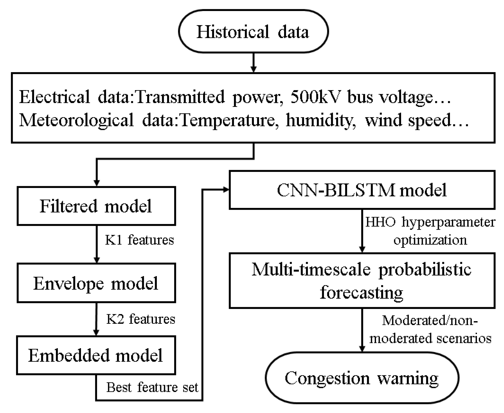
2. Joint Optimization Feature Selection Model

The prediction object of the prediction model proposed in this paper is the future grid congestion scenario of the grid, which requires the prediction of the probability values of the intervals in which the future power values of a key section of the grid are located at multiple time scales. Thus, the probabilistic results of the future scenarios of the system are obtained for proactive warning. In order to obtain quality prediction results, it is essential to screen the massive historical data of the grid in order to capture the key features that characterize the future trends. In this paper, a multi-stage joint optimization feature selection model is used to select features from the actual operational data, as well as related meteorological data of the power grid in a province in China, in order to improve the efficiency and accuracy of the prediction model.

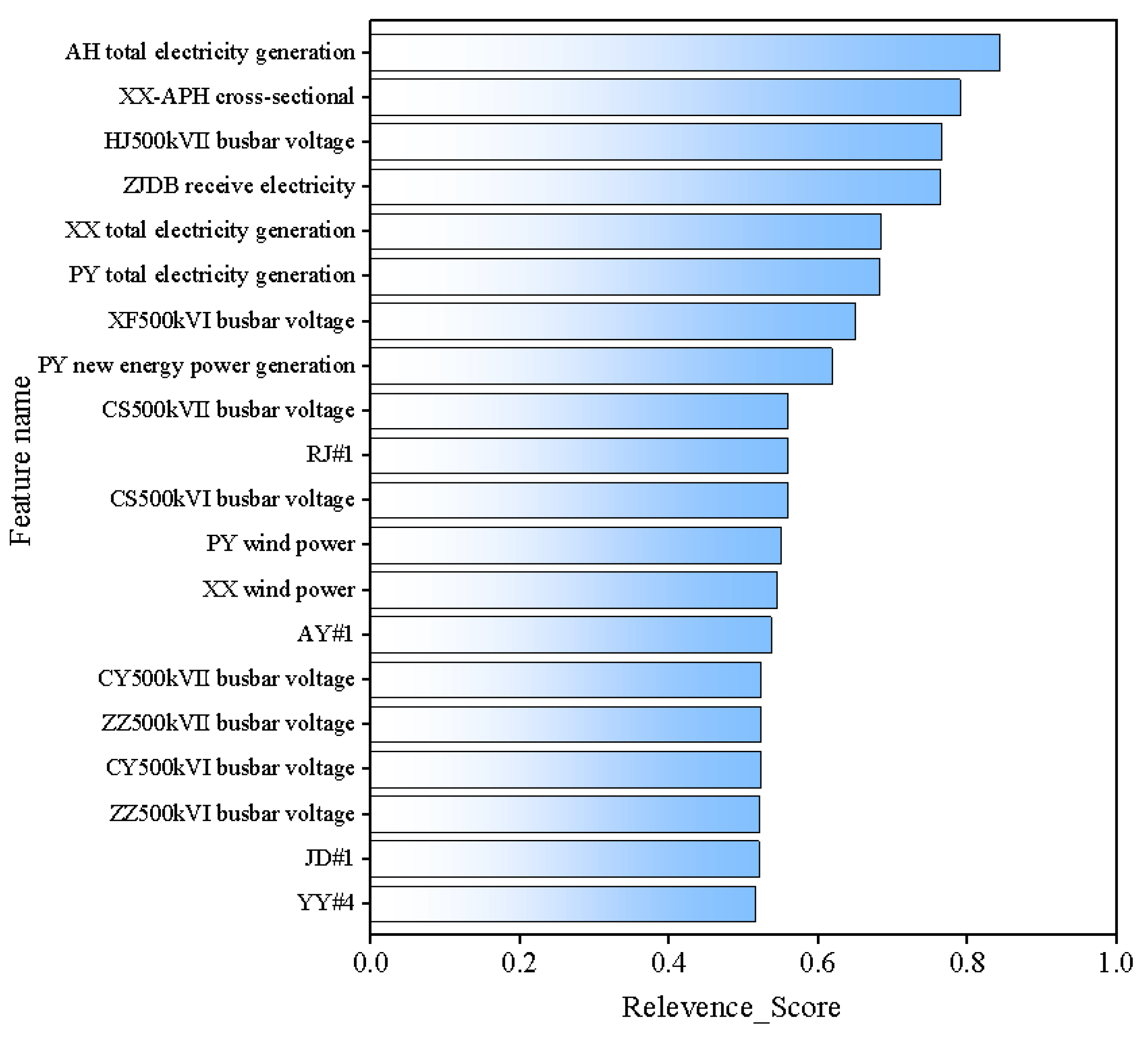
2.1. Initial Screening Phase

The actual operation data and related meteorological data of the power grid of a province in China are used as a dataset, and the dataset is divided into the feature matrix X_n×m = [x₁, x₂,…, x_a,…, x_m] and the target vector y_n×1, where 1 ≤ a ≤ m and m stands for the number of features except the target cross section and contains the electrical features and meteorological features. Each x_a is a column vector of n × 1. n represents the number of points of the recorded data, and the time interval of the data used in the paper is 5 min. For instance, if bus voltage data are collected for one hour, n is equal to 12. y represents the target cross section. Subsequently, a warning will be issued for grid congestion.

Next, the Pearson correlation coefficient matrix R_1×m = [r₁, r₂,…, r_a,…, r_m] is calculated between the feature matrix X and the target vector y. The Pearson correlation coefficient is a statistical index used to quantify the degree of linear correlation between two continuous variables, which is then used to reflect the strength and direction of the correlation between the variables through the ratio of covariance to standard deviation, with the following formula:

$$r_a={\displaystyle \frac{{\displaystyle \sum _{i=1}^n(x_{ai}-{\overline{x}}_a)(y_i-\overline{y})}}{\sqrt{{\displaystyle \sum _{i=1}^n{(x_{ai}-\overline{x_a})}^2}}\sqrt{{\displaystyle \sum _{i=1}^n{(y_i-\overline{y})}^2}}}}$$

(1)

where n denotes the number of time points included in each datum. x_ai represents the value of the ath feature at the ith time point. ${\overline{x}}_a$ and $\overline{y}$ denote the sample means of the two variables, respectively. The correlation coefficient r_a of the a-th feature takes values ranging from −1 to 1. When r is positive, it means that there is a positive correlation between the two variables, which means that one variable increases as the other increases. When r is negative, it means that there is a negative correlation between the two variables, which means that one variable increases while the other decreases. When r is 0, it means that there is no linear relationship between the two variables. And from this, the correlation coefficient between X and y in absolute form was extracted as the Pearson score.

Similarly, the Spearman correlation coefficient matrix was computed using the Spearman function. The Spearman correlation coefficient is used as a measure of the strength and direction of the monotonic relationship between the two variables, and it calculates the correlation based on the rank order of the variables instead of the raw values, as given in the following formula:

$${\rho }_a=1-{\displaystyle \frac{6{\displaystyle \sum _{i=1}^n{D}_{ai}^2}}{n(n^2-1)}}$$

(2)

where n again represents the number of time points contained in each piece of datum. D_ai represents the difference in order between the value of the ath feature at the ith time point and the value of y at the ith time point. After that, the correlation coefficient between X and y in absolute form is extracted as the Spearman score.

Finally, the absolute value scores of each feature under both Pearson and Spearman scores were summed and averaged to obtain a composite score for each X_i. Based on the composite score, the top k₁ features with the highest scores are initially selected for the subsequent fine screening stage, where the value of k₁ can be dynamically adjusted according to the size of the feature set.

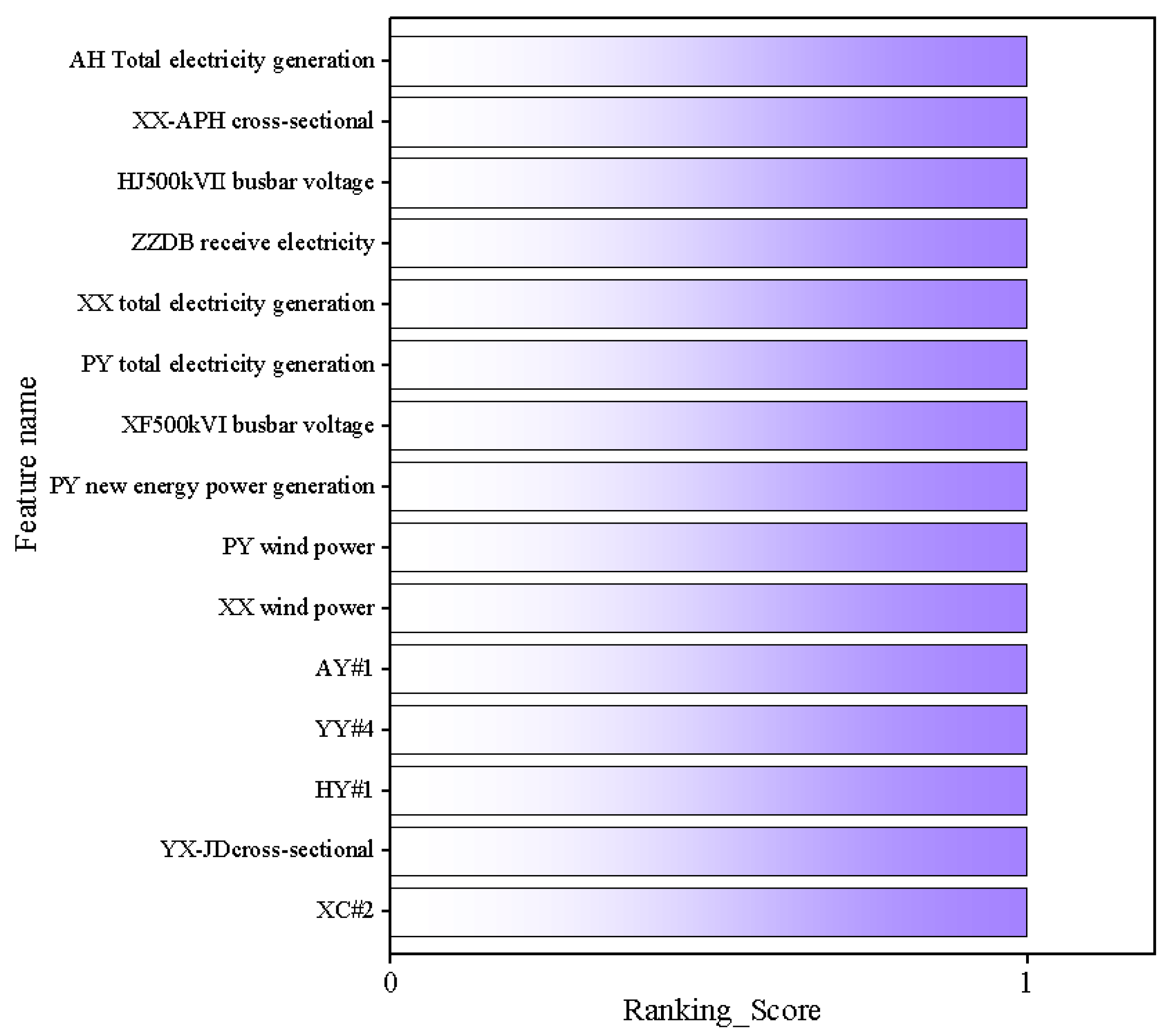
2.2. Fine Screening Phase

Similarly, the target column is taken as y, and the remaining k₁ feature columns are taken as independent variables X. We then initialize a Random Forest Regressor, which is an integrated learning method that improves the predictive performance of the model by constructing multiple decision trees and averaging their outputs. The appropriate initialization of the number of trees n₁, with random seeds n₂, can improve the computational speed while retaining high predictive performance.

Next, a Recursive Feature Elimination (RFE) selector is created, RFE is a feature selection algorithm that selects features by recursively selecting smaller and smaller sets of features. Initially, a Random Forest regression model is constructed using all the features; the importance score of each feature is calculated, and a portion of the features are progressively eliminated by sorting the features according to their importance scores from low to high. The process is repeated until the number of remaining features reaches a preset value k₂. At each step, the RFE evaluates the importance of the features using the Random Forest Regressor and calculates the score for each feature by using the following formula:

$$I_{\mathrm{importance}}(X_a)={\displaystyle \frac{1}{T}}{\displaystyle \sum _{t=1}^T\frac{L(Y,\widehat{Y_t})-L(Y,\widehat{Y_{t-a}})}{L(Y,\widehat{Y_{t.\min }})}}$$

(3)

where X_a is the ith feature, T is the number of trees in the random forest, L₁ is the prediction error of the tth tree, L₂ is the prediction error of the tth tree after excluding the ath feature, and L₃ is the prediction error of the tth tree on the smallest subset of features. The RFE algorithm outputs the ranking of each feature, where the feature with a ranking of 1 indicates the most important feature, and the further the ranking is, the lower the importance of the feature is.

Finally, the prediction performance of the subset of features selected using RFE is evaluated via cross-validation. Cross-validation is a method for assessing the generalization ability of a model by dividing the dataset into multiple subsets (If cv = 5, this means divide the data into 5 subsets for 5-fold cross-validation) and training and testing the model separately, resulting in a more stable performance assessment. The predictive performance score for each cross-validation fold is calculated, and the average predictive performance score is computed using the following formula:

$$S_{mean}={\displaystyle \frac{1}{C}}{\displaystyle \sum _{c=1}^C{S}_{cv}(c)}$$

(4)

where C is the number of cross-validation folds and S_cv(c) denotes the score of the cth cross-validation. S_mean represents the average of all cross-validation fold scores and represents the average predictive performance of the model on different data subsets. The top k₂ features of the RFE score are output to prepare for the final optimization phase.

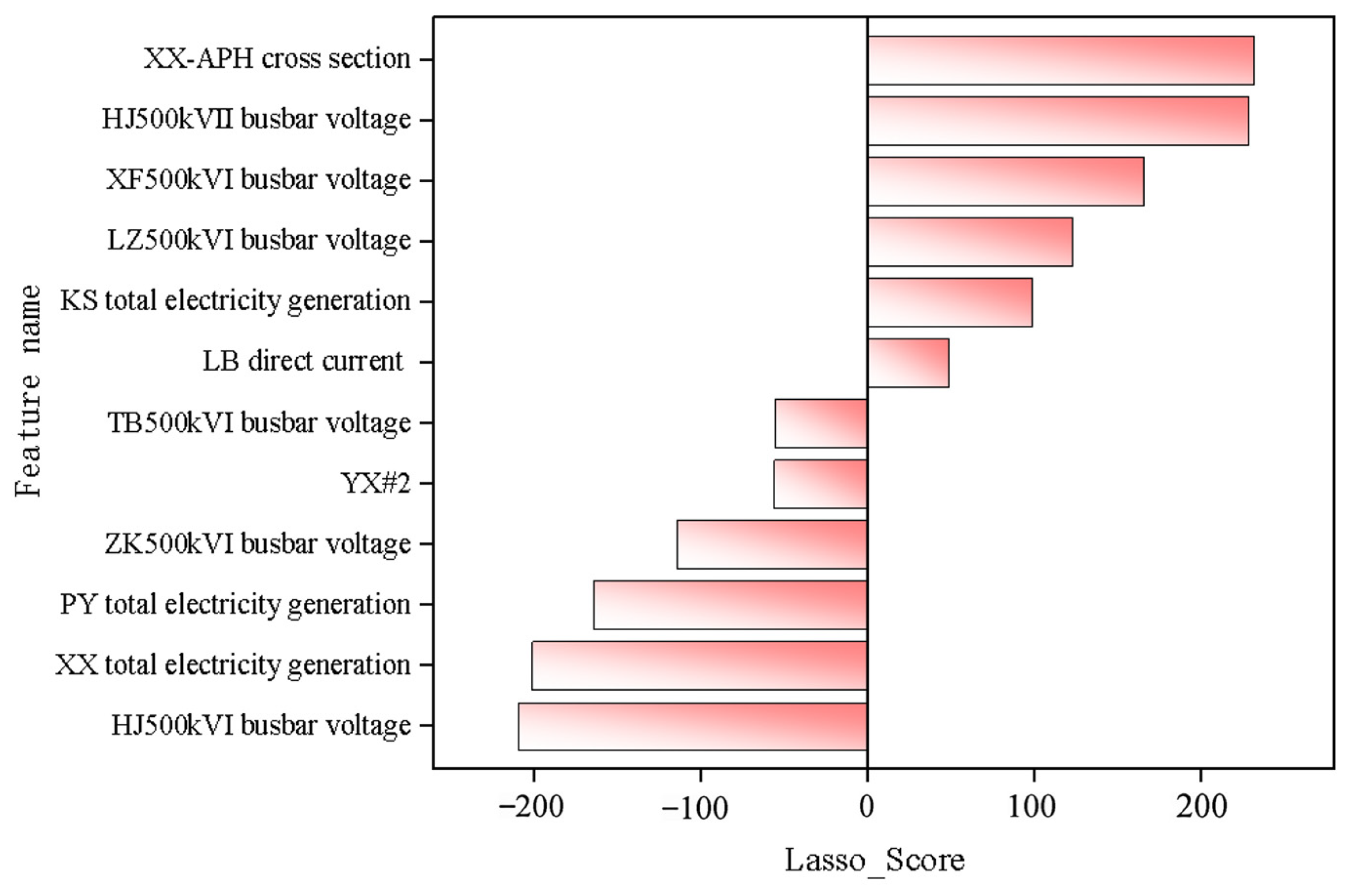
2.3. Iterative Optimization Phase

Further, Z-score normalization is performed on the target column y as well as the k₂ feature data taken in the previous section. The mean and standard deviation of each feature are first calculated, and then for each value of each feature, it is subtracted from the mean of that feature and divided by the standard deviation of that feature. The calculation formula is as follows:

$$x_{norm,i}={\displaystyle \frac{x_i-\mu }{x’}}$$

(5)

where x_i represents the ith original data in a column of data, 1 ≤ i ≤ n, and x_norm,i is its normalized data. μ is the mean of this column. x′ is the standard deviation of this column. Using the Z-score normalization method, the mean of the data is 0, while the standard deviation is 1, which makes the different features comparable to each other, and the scaled data are not affected by extreme values.

Next, the search space is defined, where the least absolute shrinkage and selection operator (LASSO) regularization parameter is searched in the interval [m₁, m₂]. The number of features is searched in the interval [f₁, k₂] to ensure that at least f₁ features are selected, and the value of f₁ can still be dynamically adjusted according to the actual situation. The objective function is constructed using the above parameters, and feature selection is performed using LASSO.

$${\min }_{\beta }\left({\displaystyle \frac{1}{2n}}{{\displaystyle \sum _{i=1}^n\left(y_i-X_i\beta \right)}}^2+\alpha {\displaystyle \sum _{j=1}^p\left|{\beta }_j\right|}\right)$$

(6)

where n is the number of samples, p is the number of features, X is the feature matrix, y is the target value of the ith sample, β is the feature coefficient to be optimized, and α is the regularization parameter, which is used to control the complexity of the model and the strictness of feature selection. Feature selection is performed using LassoCV (a module in the scikit-learn library for linear regression), which automatically selects the optimal regularization parameter α. Next, the selected subset of features is evaluated using a random forest, and the score of the model is computed through cross-validation, and the negative of the average score is returned to achieve the minimization objective. Finally, Bayesian Optimization is used to find the optimal α parameter and the number of features k₃. The LASSO model is retrained using the optimal parameters and evaluated to obtain the optimal feature subset.

3. Active Early Warning Model for Grid Congestion Based on Optimization Algorithm

The significance of the optimization algorithm is to find the best hyperparameters to help improve the performance of the prediction model. In this chapter, a prediction model based on a convolutional neural network and a bidirectional long and short-term memory network (CNN-BILSTM) will be built based on the basis of the feature selection method introduced above, while hyperparameter optimization will be carried out by using the Harris Hawks optimization (HHO) algorithm in order to improve the robustness of the prediction, which will help us obtain more accurate grid congestion prediction results.

3.1. Multi-Time-Scale Warning Model Based on CNN-BILSTM

First, the Z-score is used to standardize the k₃ features obtained from the previous section after multi-order feature selection so that the target column y has a mean of 0 and a variance of 1, which helps improve the training efficiency and convergence speed of the model. At the same time, the standardization is robust to outliers because the standard deviation is calculated while taking into account the degree of dispersion of the data points.

Next, feature reshaping is performed on the historical data, and the said historical data are converted into a 3D array.

The shape of the training set xtrain and the test set xtext was converted from a two-dimensional array to a three-dimensional array using the reshape function method to comply with the input requirements of CNN and BILSTM. Specifically, the feature data are reshaped into the shape of the number of samples, the number of time steps, and the number of features. The number of samples is kept constant. The number of time steps is set to 1, which means that the inputs are considered at a single point in time at a specific time. The number of features is k₃, which represents the selected feature data. Through data reshaping, the model can effectively handle sequence data and improve the accuracy of prediction. At the same time, this data structure can also meet the input requirements when CNN and BILSTM are used jointly, ensuring that the model runs smoothly during training and prediction.

The CNN-BILSTM model is constructed, which includes a convolutional layer, a pooling layer, a bi-directional long and short-term memory network layer, a Droopout layer, and a fully connected layer. Among them, the output of the convolutional layer can be calculated using the following equation:

$$h_i=\sigma (W_h\cdot x_i+b_h)$$

(7)

where h_i is the output of the convolutional layer, x_i is the input data, W_h is the weight of the convolutional layer, b_h is the bias, and σ is the activation function (ReLU). Local features in the sequence data are extracted by the convolutional layer to capture short-term patterns in the time series. Subsequently, the pooling layer is used to reduce the feature dimensions and reduce the computational complexity.

Next, a bidirectional long short-term memory layer is introduced to process the input data from both directions to better capture the long-term dependencies in the time series.

The formula for BILSTM is as follows:

$$h_t=\sigma \left(W_h\right[h_{t-1}{,x}_t]+b_h)$$

(8)

where h_t is the output of the forward LSTM at time point t, h_t−1 is the output of the previous time point, x_t is the input at the current time point, and W_h and b_h represent the weights and bias, respectively. σ is a sigmoid function that compresses the output value between 0 and 1.

The formula for the inverse LSTM is as follows:

$$h_t^{\prime }=\sigma (W_h^{\prime }[h_{t+1}^{\prime },x_t]+b_h^{\prime })$$

(9)

where h_t′ is the output of the inverse LSTM at time point t, h_t+1′ is the output of the previous time point, x_t′ is the input of the current time point, and W_h′ and b_h′ represent the weights and biases, respectively.

The output of the bidirectional LSTM is as follows:

$$h_t^{″}=[h_t,h_t^{\prime }]$$

(10)

where h_t″ is the final output of the BILSTM at time point t, which contains both forward and backward information.

Based on this, the Dropout layer is added for regularization to prevent overfitting and improve the generalization ability of the model. The output after applying Dropout is as follows.

$$h_t^{‴}=Dropout\left(h_t^{″}\right)$$

(11)

Finally, the probabilistic results are binary outputs that use the sigmoid activation function to obtain the probability that the sample x belongs to each category y_n.

$$\sigma (x)={\displaystyle \frac{1}{1+e^{-x}}}$$

(12)

where x is the input value and b(x) is the output value, taking values between 0 and 1. The sigmoid function ensures that the sum of the predicted probabilities of the two categories is 1 and transforms the input values into a probability distribution σ(x). The CNN-BILSTM model is trained using the dataset to obtain a preliminary dynamic prediction model of grid congestion probability.

3.2. Introduction to the HHO Principle

The HHO algorithm is insensitive to the initial conditions and can still be stable in the noise environment to find the optimal solution, making it suitable for power system optimization, machine learning hyper-parameter tuning, and other complex situations. By simulating the hunting behavior of a Harris’s Hawk, it searches for the best parameter values that can minimize the objective function in a given search space. The search space is defined here as the range of the number of BILSTM cells and the Dropout rate. There are three phases in the HHO algorithm: the global exploration phase, the global exploration to local exploitation conversion phase, and the local exploitation phase. In the HHO algorithm, the position of the Harris Hawk is treated as a candidate solution, and the best candidate solution for the iteration is the prey.

In the exploration phase, the prey is searched globally with equal probability using two strategies, when P is less than 0.5, and each eagle moves according to the other members and the prey position, and when P is greater than 0.5, Harris’s eagle randomly perches on one of the trees within the range of the population, and the position of an individual eagle is updated as follows:

$$U\left(t+1\right)=\left\{\begin{array}{ll}\left(U_{prey}\left(t\right)-U_m\left(t\right)\right)-{rand}_3\left(lb+{rand}_4\left(ub-lb\right)\right)\hfill & ,P<0.5\hfill \\ U_{rand}\left(t\right)-{rand}_1\left|U_{rand}\left(t\right)-2{rand}_{2}U\left(t\right)\right|\hfill & ,P\ge 0.5\hfill \end{array}\right.$$

(13)

where U(t + 1) is the position of an individual hawk in the t + 1st iteration, i.e., the position at the next moment; U_prey(t) is the position of the prey in the tth iteration; U_rand(t) is the position of a randomly selected individual Harris’s hawk in the tth iteration; U_m(t) is the average position of an individual hawk in the tth iteration; ub and lb are, respectively, the upper and lower bounds of the search upper and lower bounds of the space; and rand₁, rand₂, rand₃, and rand₄ are random numbers in the interval (0, 1).

In the exploration–exploitation transition phase, since the energy of the prey decreases during the escape process, a linearly decreasing formula modeling the decrease in prey energy is used, and the prey escape energy is defined as follows:

$$E=2E_0(1-{\displaystyle \frac{t}{M}})$$

(14)

where E₀ is the initial escape energy of the prey, which is a random number between (−1, 1); t is the current evolutionary generation; and M is the maximum evolutionary generation of the population. The exploration phase is entered when |E| ≥ 1, and the exploitation phase is entered when |E| < 1.

In the exploitation phase, the Harris’s Hawk launches an attack after finding the target prey. The HHO employs four strategies, namely soft encirclement, hard encirclement, soft encirclement with progressive fast swooping, and hard encirclement with progressive fast swooping, to mimic the Harris Hawk’s hunting behavior.

S_p is defined as the prey escape probability, and it is a random number between (0, 1). S_p < 0.5 means there is a chance of escape. The hunting strategies are determined by combining the prey escape energy |E| and the prey escape probability S_p.

When 0.5 ≤ |E| < 1 and S_p ≥ 0.5, the prey still has energy to escape and tries to escape the encirclement through random jumps. At this point, the hawk uses a soft encirclement to prey on the prey to exhaust it, thus allowing the hawk to make a surprise raid.

$$U\left(t+1\right)=\Delta U\left(t\right)-E\left|J{U}_{prey}\left(t\right)-U\left(t\right)\right|$$

(15)

$$\Delta U\left(t\right)=U_{prey}\left(t\right)-U\left(t\right)$$

(16)

where U(t) is the difference between the prey position and the current individual position during the tth iteration; J-U is in the range of (0, 2).

When |E| < 0.5 and S_p ≥ 0.5, the prey has no energy to escape, so there is no chance of escape. The Harris’s hawk uses hard encirclement to prey on the prey in order to make a final surprise raid with the updated equation.

$$U\left(t+1\right)=\Delta U\left(t\right)-E\left|J{U}_{prey}\left(t\right)-U\left(t\right)\right|$$

(17)

When 0.5 ≤ |E| < 1 and S_p < 0.5, the prey has a chance to escape from the encirclement and has enough energy to escape from the hawk’s capture. However, the Harris’s hawk will surround the prey with a gradual, fast swooping soft encirclement, gradually correcting its position and direction according to the prey’s deceptive behavior so as to choose the optimal position to capture the prey, which is implemented using the following two strategies. When the first strategy is ineffective, the second strategy is implemented with the updated formula.

$$U\left(t+1\right)=\left\{\begin{array}{ll}Y=U_{prey}\left(t\right)-E\left|J{U}_{prey}\left(t\right)-U\left(t\right)\right|\hfill & ,if\hspace{0.33em}F\left(Y\right)<F\left(U\left(t\right)\right)\hfill \\ Z=Y+S\times Le\prime vy\left(D\right)\hfill & ,if\hspace{0.33em}F\left(Z\right)<F\left(U\left(t\right)\right)\hfill \end{array}\right.$$

(18)

F() is the fitness function. S is a d-dimensional random vector with elements between (0, 1). Le’vy is the Lévy flight strategy, which is given by the formula as follows.

$$L{e}^{\prime }vy=0.01\times {\displaystyle \frac{u\times \sigma }{{\left|v\right|}^{\frac{1}{\beta }}}},\sigma ={\left({\displaystyle \frac{\mathit{\Gamma }\left(1+\beta \right)\times \sin \left(\frac{\pi \beta }{2}\right)}{\mathit{\Gamma }\left(\frac{1+\beta }{2}\right)\times \beta \times 2\left(\frac{\beta -1}{2}\right)}}\right)}^{{\displaystyle \frac{1}{\beta }}}$$

(19)

When |E| < 0.5 and S_p < 0.5, the prey is exhausted but still has a chance to escape. The Harris’s Hawks hard encircle the prey through progressively faster dives. This strategy allows the hawks to update their position formula similar to that in soft encirclement through progressively faster dives. In this case, the Harris’s hawks try to reduce their distance from the mean position of the target prey with an updated formula.

$$U\left(t+1\right)=\left\{\begin{array}{ll} Y=U_{prey}\left(t\right)-E\left|J{U}_{prey}-U_m\left(t\right)\right|\hfill & ,if\hspace{0.33em}F\left(Y\right)<F\left(U\left(t\right)\right)\hfill \\ \hspace{0.33em}Z=Y+S\times L{e}^{\prime }vy\left(D\right)\hfill & ,if\hspace{0.33em}F\left(Z\right)<F\left(U\left(t\right)\right)\hfill \end{array}\right.$$

(20)

Further, in the process of training the CNN-BILSTM model using the dataset, the attention mechanism is introduced to focus on the part of the input sequence that has the greatest impact on the prediction results.

In this case, the formula for the attention mechanism is as follows:

$${\alpha }_t={\displaystyle \frac{\exp \left(e_t\right)}{{\displaystyle {\sum }_{i=1}^T\exp \left(e_t\right)}}}$$

(21)

where e_t is the attention score at time point t and α_t is the attention weight. e_t is expressed as follows:

$$e_t=\tan \mathrm{h}(W_e\cdot [h_t^{‴},h_t^{‴}]+b_e)$$

(22)

where W_e and b_e are the weight and bias of the attention layer, respectively.

Finally, a weighted summation is performed with the following equation:

$$c_i={\displaystyle {\sum }_{i=1}^T}{\alpha }_i\cdot h_t^{″}$$

(23)

where c_i is the weighted context vector and h_t″ is the output of the BILSTM.

Finally, the best feature dataset obtained through the multi-stage joint optimization feature selection method above is imported into this prediction model, which can predict the grid congestion probability of a key section of the grid, thus realizing active warning.

4. Example Analysis

In order to verify the effectiveness of the proposed method, this paper selects the above historical data of a provincial network in China, which is the hub of the national interconnected grid and one of the power resource distribution centers and is directly related to the safe and stable operation of the national grid. The data starting point is 1 March 2021, and the end point is 1 March 2022. In the data processing process, the time interval of the data is 5 min/time, considering that the subsequent multi-time-scale prediction covers the hourly period. A representative typical grid congestion event was selected for the arithmetic test.

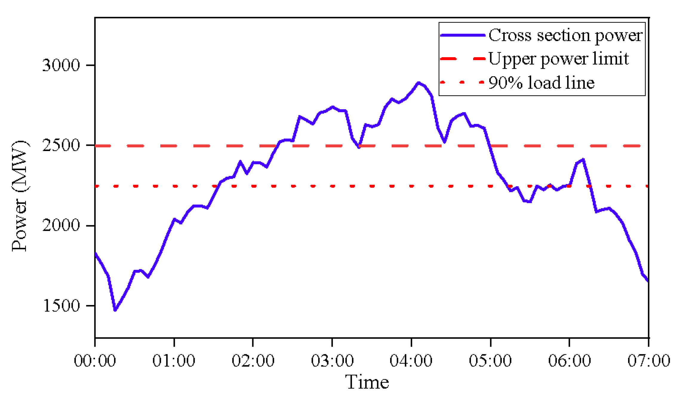
4.1. Definition of Grid Congestion Events

Grid congestion refers to the capacity limitations of the transmission line in the power system, that is, the transmission of power more than the line can withstand. Grid congestion leads to the transmission of electric energy that cannot meet the requirements of the supply and demand balance, which in turn triggers the line heavy load and even leads to line power over the line, seriously affecting the stable operation of the power system. The line loading factor (LLF) is calculated as follows:

$$\mathrm{LLF}={\displaystyle \frac{S_a}{S_{a,\max }}}$$

(24)

where S_a is the transmission power of line a. S_a,max is the transmission power limit of line a, which is set in accordance with the relevant power system security and stability regulations. And the transmission power limit in this paper is given by the dispatching department. In this paper, the points with a load ratio greater than 90% are set as heavy load points, and the future scenarios are divided into regulation scenarios and non-regulation scenarios based on whether the heavy load points appear or not, as shown in

Table 1. Future scenario categories.

LLF	≤90%	>90%
categories	Non-regulatory Scenarios	Regulation scenarios
tab	0	1

.

The feature selection and prediction part of this chapter will be categorized according to the divisions shown in Table 1. Of course, it is also possible to continue the study according to other classifications depending on the characteristics of the grid.

4.2. Multi-Stage Feature Selection Model Construction

In this paper, actual load data and meteorological data collected from a province in China are utilized as the data sources. The data are input into a multi-stage joint optimization feature selection model. In this paper, electrical data with a time span of 365 days and a time interval of 5 min, as well as meteorological six-factor data, totaling 622 feature data, are used, which fully consider the influencing factors of the target area in one year. And a total of 191 grid congestion events occurred in the region in the fourth quarter of 2021, with more than 50% of the key cross sections having congestion events and even serious problems of power overruns. Taking the YZ-YB cross section as an example, as a key transmission cross section in the central–northern part of the province, nearly 80 grid congestion events occurred in three months, and the cross section congestion problem is very prominent. In this paper, the YZ-YB cross section is selected as the research object. It explores the influence of transmission power of the rest of the cross section, line transmission power, the power generation of each new energy source, and meteorological factors such as temperature and humidity with the transmission power of this cross section. Through the multi-stage feature selection model, the most optimal set of features that helps to predict the future congestion of the YZ-YB section is gradually obtained. The overall idea is shown in Figure 1.

Firstly, this paper processed the original dataset for missing values and outliers and performed time alignment and resampling to correct the accuracy of the data. In the preliminary screening stage of feature selection, this paper combines two correlation analysis algorithms, Spearman and Pearson, to comprehensively evaluate the electrical and meteorological features from linear and nonlinear perspectives. According to the scoring threshold, the first k₁ feature data (this paper takes k₁ = 100) are retained in order to quickly filter the obviously irrelevant feature data and reduce the complexity of the calculation. Some of the feature data results are shown in Figure 2.

Further, in the fine screening stage of feature selection, the features are first ranked using Recursive Feature Elimination combined with a Random Forest. Then, these features are evaluated via cross-validation, and the top k₂ features are retained (in this paper, we take k₂ = 50) in order to further filter out the features that have a significant impact on the model performance. The top k₂ features are all ranked as one. Some of the feature data results are shown in Figure 3.

In the optimization stage of feature selection, the Z-score is used to standardize the scaling of the features so that different features are comparable and not affected by extreme values. Then, LassoCV is used for feature selection, while Bayesian Optimization is used to obtain the optimal parameters. Finally, a Random Forest is utilized for evaluation to obtain the optimal subset of features (k₃ = 12 in this paper), and the optimal feature set is shown in Figure 4. Among them, the sizes of k₁ and k₂ can all be adjusted according to the actual data size of the features, while the size of k₃ is the optimal value obtained via RF iterative optimization search.

4.3. Probabilistic Prediction Model Construction

After the feature selection model is constructed, the prediction model can be further constructed. Since this paper divides the future scenarios based on a 90% loading rate, the target column y needs to be preprocessed before prediction. The value of S_b,max for the YZ-YB section that is greater than 90% is marked as one; otherwise, it is marked as zero. During the construction of the probabilistic prediction model, a search space containing the number of LSTM cells and the Dropout rate is defined in order to optimize the hyperparameters of the model. Then, cross-validation as well as grid search is used to divide the dataset into five mutually exclusive subsets, each of which in turn serves as a test set, and the remaining subsets serve as a training set for model training and validation to assess the generalization ability of the model. In each cross-validation fold, the training set is further divided into a training subset and a validation subset, and the validation subset accounts for 20% of the training set. The HHO algorithm is used to find the optimal hyperparameters within the defined search space, after which these hyperparameters are used to train the optimized CNN-BILSTM model with EarlyStopping callbacks to prevent overfitting.

For the probabilistic classification problem of grid congestion, the proposed algorithm is compared with other machine learning algorithms in terms of computational efficiency and accuracy using a sample set of data, which includes a support vector machine (SVM), logistic regression (LR), K-nearest neighbors (KNs).

Table 2. Comparison between different machine learning algorithms.

Algorithm	Accuracy	Training Time/s	Prediction Time/s
SVM	0.83	78.24	2.76
LR	0.74	29.20	0.92
KN	0.71	2.46	2.33
RF	0.84	30.55	0.79
CNN-BILSTM	0.88	15.81	0.81

shows the accuracy of the grid congestion binary classification prediction for different algorithms on a 30 min time scale, as well as the time required for one training and prediction session using the data, where the accuracy is the mean of the ratio of the number of samples classified correctly by the prediction model in the test dataset to the number of all samples in the test dataset.

Compared to other algorithms, the proposed algorithm has the highest accuracy, with an average accuracy of 0.88 in cross-validation. In terms of training time, CNN-BILSTM also pairs good training speed with faster prediction time. Efficient training allows CNN-BILSTM to update the model in real-time problems in a timely manner to improve adaptability.

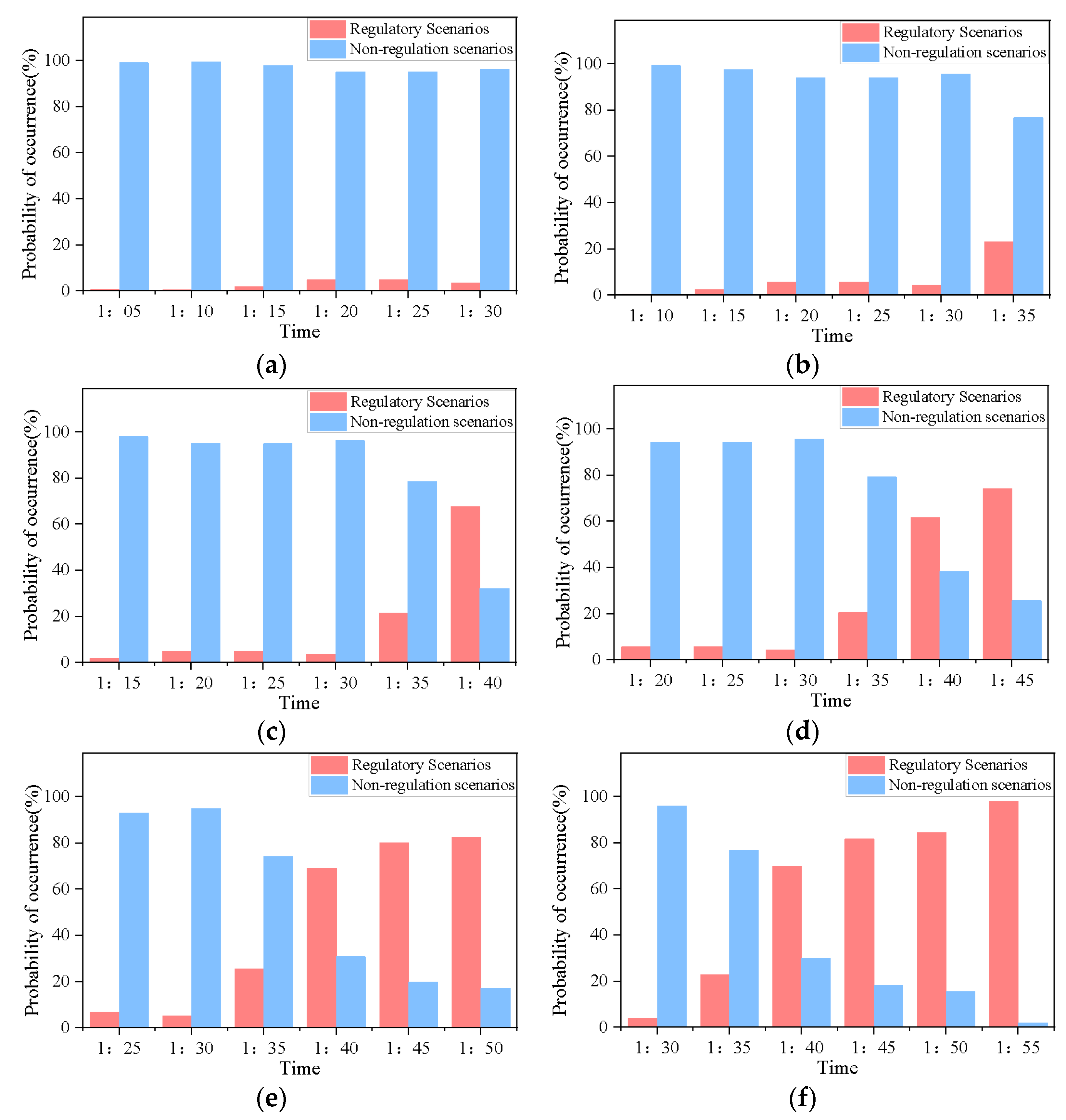
4.4. Active Warning Results Based on Multiple Time Scales

After the construction of the probabilistic prediction model is completed, grid congestion active warning can be verified. In this paper, the grid congestion event that occurred in the early morning of 10 November 2021 at the above YZ-YB section is selected for prediction and analysis. Since the research content of this paper mainly focuses on the real-time operation of the power grid to provide active warning, the warning results can be used for subsequent grid regulation and mitigation, so the intra-hour prediction is selected as the main research content. Taking half an hour as the time scale as an example, the single-time-scale prediction model must take 30 min as a prediction time scale, input the actual data at 01:00, and only output the prediction data at 01:30. The multi-time-scale prediction model, however, can predict six time nodes based on the actual data at 01:00, 01:05, 01:10…01:25, and 01:30, respectively, with six time scales. Obviously, the multi-time-scale prediction can provide a certain prediction horizon while ensuring the real-time prediction in short time scales, which improves the applicability and robustness of the model.

Figure 5 demonstrates the power change curve of the YZ-YB section during the 10 November 2021 grid congestion event. It can be seen that the YZ-YB section started to show power crossing the line at about 02:25, which continued to increase within the next half hour, although it temporarily decreased at about 03:15, but it still showed nearly two hours of crossing the line, which seriously affects the operation safety of the power system. However, if future grid congestion can be detected before the section power crosses the line and control measures can be taken in time, it is expected to alleviate or avoid the occurrence of this grid congestion event.

In this paper, we set out to predict the probability of grid congestion at multiple time scales for 01:00 and beyond. When the predicted probability of grid congestion at a future time point is greater than 50%, the moment is considered as a regulation scenario; otherwise, it is a non-regulation scenario. According to the prediction results in Figure 6, after 01:00 hrs, the probability of future regulation scenario increases as time passes, and according to the development trend of the multi-time-scale prediction, after 01:35 hrs, the grid will be changed from a non-regulation scenario to a regulation scenario in the future. According to the warning result in Figure 6d, at 01:35, the warning result is a non-regulation scenario (the probability of a non-regulation scenario is greater than 50%), but it should actually be a regulation scenario, and there is an error in judging the grid congestion category, and the warning situation slightly lags behind the real situation. However, the dispatcher can analyze the real trend of grid congestion by combining the multi-time-scale probabilistic prediction graphs. After 01:30, the probability of the non-regulation scenario gradually decreases, and the probability of the regulation scenario gradually rises, so the grid is very likely to develop into a regulation scenario by 01:35.

This early warning results with probability trend analysis can provide scheduling personnel with intuitive category results and a congestion trend analysis basis. Based on the congestion warning results in multiple time scales, the scheduler can issue different time-scale regulation strategies. The long-time-scale strategy makes full use of controllable resources with a low cost and a slow response time. The short-time-scale strategy completes the complement of the strategy to ensure the effectiveness and reliability of congestion clearance. In this way, it improves the scheduler’s ability to judge the overall situation of power system congestion and ensures the safe operation of the power system.

5. Conclusions and Prospectives

In this paper, we construct an active warning model for grid congestion considering probabilistic prediction, implement a CNN-BILSTM multi-time-scale probabilistic prediction model based on multi-order joint optimal feature selection and HHO algorithm optimization, and ultimately transform it into a binary warning result for grid congestion so as to guide active regulation. The effectiveness of the method proposed in this paper and the accuracy of the prediction model are verified through examples.

(1).

The model is able to filter out the optimal feature set based on historical data, thus improving the prediction efficiency and accuracy of the prediction model. At the same time, the data-driven approach avoids the drawbacks of the traditional parametric model that is affected by the system operation mode and enhances the robustness of the prediction model.

(2).

While providing probabilistic outputs and early warning results, the model adopts a multi-time-scale prediction approach, thus providing more valuable information for dispatchers to make auxiliary decisions and help the operational safety of the power system.

(3).

In this paper, during the feature selection process, only the correlation between the feature set and the requested features is considered, and the interactions within the feature set are not taken into account, which may weaken the potential impact of certain features. Therefore, subsequent attempts will be made to explore the synergistic or antagonistic effects between features to further improve the representativeness of the selected features.

(4).

This paper focuses on the early warning of the future grid congestion probability of the power system, thus guiding active regulation, and in the subsequent work, the specific regulation strategy can be further considered to improve grid congestion early warning and active regulation so as to carry out a more comprehensive active regulation strategy development.

References

1. Sun, Y.Z.; Wu, J.; Li, G.J.; He, J. Development models and key technologies of future grid in China. Proc. CSEE 2014, 34, 4999–5008. [Google Scholar]
2. Sun, Y.Z.; Wu, J.; Li, G.J.; He, J. Dynamic economic dispatch considering wind power penetration based on wind speed forecasting and stochastic programming. Proc. CSEE 2009, 29, 41–47. [Google Scholar]
3. Sha, Y.; Qiu, X.; Ning, X.; Han, X. Multi-objective optimization of active distribution network by coordinating energy storage system and flexible load. Power Syst. Technol. 2016, 40, 1394–1399. [Google Scholar]
4. Lu, W.; Du, H.; Ding, Q.; Tu, M.; Li, W.; Ji, W. Design and key technologies of optimal dispatch for smart distribution network. Autom. Electr. Power Syst. 2017, 41, 1–6. [Google Scholar]
5. Liu, Q.; Li, J.; Ni, M. Situation awareness of grid cyber-physical system; current status and research ideas. Autom. Electr. Power Syst. 2019, 43, 9–21. [Google Scholar]
6. Wang, C.; Luo, F.; Zhang, T. Review on key technologies of smart urban power network. High Volt. Eng. 2016, 42, 2017–2027. [Google Scholar]
7. Huang, M.; Wei, Z.; Sun, G.; Zang, H.; Huang, Q. A novel situation awareness approach based on historical data mining model in distribution networks. Power Syst. Technol. 2017, 41, 1139–1145. [Google Scholar]
8. Li, B.Q.; Liu, D.W.; Qin, X.H.; Yan, J.F. Concept and theory framework of panoramic security defense for bulk power system driven by information. Proc. CSEE 2016, 36, 5796–5805. [Google Scholar]
9. Xu, C.; Liang, R.; Cheng, Z.; Xu, D. Security situation awareness of smart distribution grid for future energy internet. Electr. Power Autom. Equip. 2016, 36, 13–18. [Google Scholar]
10. Zhu, Q.; Dang, J.; Chen, J.; Xu, Y.; Li, Y.; Duan, X. A method forpower system transient stability assessment based on deep belief networks. Proc. CSEE 2018, 38, 735–743. [Google Scholar]
11. Dai, Y.; Chen, L.; Zhang, W.; Min, Y.; Li, W. Power system transient stability assessment based on multi-support vector machines. Proc. CSEE 2016, 36, 1173–1180. [Google Scholar]
12. Hu, W.; Zheng, L.; Min, Y.; Dong, Y.; Yu, R.; Wang, L. Research on power system transient stability assessment based on deep learning of big data technique. Power Syst. Technol. 2017, 41, 3140–3146. [Google Scholar]
13. Duan, B.; Chen, M.; Li, H.; Lai, J. Decision method of proactive operation for distributed generation based on power quality situation awareness. Autom. Electr. Power Syst. 2016, 40, 176–181. [Google Scholar]
14. Mccalley, J.D.; Vitta, L.V. An overview of risk based security assessment. In Proceedings of the IEEE Power Engineering Society Summer Meeting, Edmonton, AB, Canada, 18–22 July 1999. [Google Scholar]
15. Kirschen, D.S.; Jayaweera, D. Comparison of risk based and deterministic security assessments. IET Gener. Transm. Distrib. 2007, 1, 527–533. [Google Scholar] [CrossRef]
16. McCalley, J.; Fouad, A.; Vittal, V.; Irizarry-Rivera, A.; Agrawal, B.; Farmer, R. A risk based security index for determining operating limits in stability limited electric power systems. IEEE Trans. Power Syst. 1997, 12, 1210–1219. [Google Scholar] [CrossRef]
17. Ni, M.; McCalley, J.D.; Vittal, V.; Tayyib, T. Online risk based security assessment. IEEE Trans. Power Syst. 2003, 18, 258–265. [Google Scholar] [CrossRef]
18. Hu, S.; Chao, Z.; Zhong, H. Modeling and application of power grid dispatching operation risk consequences. Autom. Electr. Power Syst. 2016, 40, 54–60. [Google Scholar] [CrossRef]
19. Chen, W.H.; Jiang, Q.Y.; Cao, Y.J.; Han, Z.X. Risk assessment of voltage collapse in power system. Power Syst. Technol. 2005, 29, 6–11. [Google Scholar]
20. Shi, H.J.; Ge, F.; Ding, M.; Zhang, R.L.; Huang, D.; Xu, T.; Lin, H. Research on online assessment of transmission network operation risk. Power Syst. Technol. 2005, 29, 43–48. [Google Scholar]
21. Qiu, W.; Zhang, J.; Liu, N.; Zhu, X.; Liu, L. Multi-objective optimal generation dispatch with consideration of operation risk. Proc. CSEE 2012, 32, 64–72. [Google Scholar]
22. Yu, Y.; Wang, D. Dynamic security risk assessment and optimization of transmission systems. Sci. China 2009, 39, 286–292. [Google Scholar] [CrossRef]
23. Chen, W.H. Risk-Based Security Analysis and Preventive Control in Power System. Ph.D. Thesis, Zhejiang University, Hangzhou, China, 2007. [Google Scholar]
24. Jiang, Y.; Mccalley, J.D.; Voorhis, T.V. Risk-based resource optimization for transmission system maintenance. IEEE Trans. Power Syst. 2006, 21, 1191–1200. [Google Scholar] [CrossRef]
25. Veeramsetty, V.; Reddy, K.R.; Santhosh, M.; Mohnot, A.; Singal, G. Short-term electric power load forecasting using random forest and gated recurrent unit. Electr. Eng. 2022, 104, 307–329. [Google Scholar] [CrossRef]
26. Ahmad, T.; Manzoor, S.; Zhang, D. Forecasting high penetration of solar and wind power in the smart grid environment using robust ensemble learning approach for large-dimensional data. Sustain. Cities Soc. 2021, 75, 103269. [Google Scholar] [CrossRef]
27. Eseye, A.T.; Zhang, J.; Zheng, D. Short-term photovoltaic solar power forecasting using a hybrid Wavelet-PSO-SVM model based on SCADA and Meteorological information. Renew. Energy 2018, 118, 357–367. [Google Scholar] [CrossRef]
28. Nam, S.; Hur, J. Probabilistic forecasting model of solar power outputs based on the naive Bayes classifier and kriging models. Energies 2018, 11, 2982. [Google Scholar] [CrossRef]
29. Wang, J.; Li, P.; Ran, R.; Che, Y.; Zhou, Y. A short-term photovoltaic power prediction model based on the gradient boost decision tree. Appl. Sci. 2018, 8, 689. [Google Scholar] [CrossRef]
30. Xu, J.; Jiang, X.; Liao, S.; Ke, D.; Sun, Y.; Yao, L.; Mao, B. Probabilistic prognosis of wind turbine faults with feature selection and confidence calibration. IEEE Trans. Sustain. Energy 2023, 15, 52–67. [Google Scholar] [CrossRef]
31. Memmel, E.; Steens, T.; Schlüters, S.; Völker, R.; Schuldt, F.; Von Maydell, K. Predicting renewable curtailment in distribution grids using neural networks. IEEE Access 2023, 11, 20319–20336. [Google Scholar] [CrossRef]
32. Sharma, S.; Srivastava, L. Prediction of transmission line overloading using intelligent technique. Appl. Soft Comput. 2008, 8, 626–633. [Google Scholar] [CrossRef]
33. Balaraman, S.; Kamaraj, N. Cascade BPN based transmission line overload prediction and preventive action by generation rescheduling. Neurocomputing 2012, 94, 1–12. [Google Scholar] [CrossRef]
34. Almassalkhi, M.R.; Hiskens, I.A. Model-predictive cascade mitigation in electric power systems with storage and renewables—Part I: Theory and implementation. IEEE Trans. Power Syst. 2014, 30, 67–77. [Google Scholar] [CrossRef]
35. Kalogeropoulos, I.; Sarimveis, H. Predictive control algorithms for congestion management in electric power distribution grids. Appl. Math. Model. 2020, 77, 635–651. [Google Scholar] [CrossRef]
36. Jibran, M.; Nasir, H.A.; Qureshi, F.A.; Ali, U.; Jones, C.; Mahmood, I. A demand response-based solution to overloading in underdeveloped distribution networks. IEEE Trans. Smart Grid 2021, 12, 4059–4067. [Google Scholar] [CrossRef]
37. Liao, S.; Liu, Y.; Xu, J.; Jia, L.; Ke, D.; Jiang, X. Data-Driven Real-Time Congestion Forecasting and Relief with High Renewable Energy Penetration. IEEE Trans. Ind. Inform. 2024, 21, 12–29. [Google Scholar] [CrossRef]
Figure 1. Structure of grid congestion warning based on feature selection.
Energies 18 02530 g001
Figure 2. Partial results of the initial screening phase.
Energies 18 02530 g002
Figure 3. Partial results of the fine screening stage.
Energies 18 02530 g003
Figure 4. Optimization stage best feature solicitation.
Energies 18 02530 g004
Figure 5. Actual power curve for YZ-YB section during a blockage event.
Energies 18 02530 g005
Figure 6. Multi-time-scale active probability prediction results at different times: (a) 1:00; (b) 1:05; (c) 1:10; (d) 1:15; (e) 1:20; and (f) 1:25.
Energies 18 02530 g006