An Interpretable Data-Driven Dynamic Operating Envelope Calculation Method Based on an Improved Deep Learning Model

Abstract

As the integration of distributed energy resources (DERs) continues to rise, the simultaneous import and export of energy can lead to excessive voltage violations. Therefore, calculating dynamic operating envelopes (DOEs), which represent time-varying export restrictions, is essential for ensuring the safe operation of distribution networks. Traditional methods for calculating DOEs rely on complete distribution network parameters for power-flow calculations. However, acquiring accurate parameters and network topology is often challenging, which limits the practical implementation of these traditional approaches. This paper proposes an interpretable model-free DOE calculation method that leverages smart meter data to address this issue. We train a CNN-LSTM-Attention neural network for voltage estimation, where we employ the whale optimization algorithm (WOA) to adjust hyperparameters automatically. Additionally, this paper employs the SHAP algorithm to interpret the deep learning model, providing insights into the relationship between the bus voltage and the condition of each bus, which enhances the model’s transparency and helps identify the key factors influencing voltage levels. The proposed method is validated through simulations on the IEEE 33−bus distribution network model, demonstrating favorable results.

1. Introduction

In recent years, the growing adoption of distributed energy resources (DERs), including photovoltaic systems, battery storage, and electric vehicles, has significantly altered the operation of distribution grids [1]. These technologies have enabled end users to transition from passive consumers to active participants in electricity generation, contributing to the grid and engaging in energy markets. However, this also raises safety concerns. Simultaneous energy export by DERs can lead to critical issues, such as voltage overruns [2].

To address security concerns, traditional methods typically establish static limits for each DER, restricting energy exports from each bus to ensure the safe operation of the distribution network. However, this approach can result in the underutilization of energy, significantly wasting available export capacity. A promising solution involves calculating dynamic operating envelopes (DOEs) [3,4,5], which define time-varying limits for power output and input at various buses within the network. According to [6], an operating envelope is described as “a convex set that defines the active and reactive power that can be transmitted to and from the network at a given customer connection point or group of customers in a region”. Typically, a dynamic operating envelope is determined using traditional active network management methods [7] or optimal tidal current calculation approaches [8,9]. These studies often incorporate voltage and thermal overload limits as performance constraints when calculating DOEs [5]. Some methods employ iterative techniques to estimate DOEs, considering bus voltage constraints [10], while others apply distributed strategies such as the Alternating Direction Method of Multipliers (ADMM) to allocate DOEs [6]. To address the uncertainty in generation and forecasting, which impacts DOEs and capacity allocation, the concept of the Robust DOE (RDOE) was introduced in [11]. Furthermore, DOEs have been integrated into tiered frameworks to assess BER capacity, offering consumers flexibility to operate at any point within the calculated envelope [12]. Additionally, cooperative game theory combined with DOEs has been used to design a network-aware peer-to-peer (P2P) trading scheme that enhances energy exchange between prosumers and distribution networks [13]. A decentralized P2P grid energy trading mechanism, incorporating DOEs, has also been proposed to prevent network violations [14].

However, the OPF-based approaches presented in these studies face challenges when scaled to real-world networks, as they require direct access to all DERs [15] and often suffer from computational complexity and non-convergence issues [16,17,18]. In addition, these methods typically rely on power-flow analysis to calculate the voltage, which requires accurate distribution network parameters and detailed electrical models [5]. Unfortunately, obtaining accurate data on distribution network topology and parameters such as line impedance is challenging with existing technology [19]. As a result, acquiring these electrical models is both costly and resource-intensive. Therefore, many researchers have tried to utilize data-driven approaches rather than model-based approaches.

The advancement of artificial intelligence (AI) and the widespread adoption of smart meters have created new opportunities for DOE calculations. AI technology has already been extensively applied in power systems, including load forecasting, fault diagnosis, and frequency regulation, by leveraging data-driven approaches to build deep learning models and extract insights from large datasets [20]. Simultaneously, deploying smart meters provides distribution companies with real-time data on the voltage, current, and power factor, offering a rich source of information to support data-driven methods [21]. As a result, data-driven approaches are gradually emerging as a viable alternative to traditional model-based approaches. Recent research has explored various approaches to leveraging artificial intelligence in distribution networks. Some studies employ methods such as linear regression and Gaussian processes to establish relationships between monitoring data and system voltage [22,23]. Others utilize advanced deep learning techniques, including random forests (RF), multilayer perceptrons (MLPs), long short-term memory (LSTM) networks, convolutional neural networks (CNNs), and radial basis function (RBF) neural networks, to model system states based on monitored data [24,25,26,27]. These efforts provide a robust theoretical foundation for model-free approaches to calculating DOEs.

Research on model-free methods for calculating DOEs remains limited, mainly due to the complexity of linking DOEs with monitoring data in a model-free environment. This challenge arises because DOE calculations involve not only state estimation at the bus level in the distribution network but also the consideration of system-level constraints. In [28], methods for calculating DOEs without relying on electrical models were proposed. These methods use historical data from end-customer smart meters to train a neural network (NN) that establishes the relationship between inputs and outputs. The trained neural network, combined with a heuristic algorithm, is then used to compute the operational envelope based on a selected allocation policy. A similar model-free approach, using Deep Reinforcement Learning (DRL) for real-time voltage regulation in active distribution networks, was presented in [29,30]. However, one significant limitation of black-box models and machine learning (ML) techniques is their lack of interpretability. The outputs generated by these models do not always provide a clear explanation of how they were derived. While neural networks are trained on historical data and various algorithms to capture patterns and variations, they can produce inaccurate results when exposed to conditions not encountered during training. This issue arises because the model may not have encountered such variations during the training phase, leading to deviations from the expected output.

In this paper, an interpretable deep learning model is constructed for voltage computation, which is based on a CNN-LSTM architecture, combined with WOA and an attention mechanism to improve the performance of the model. Moreover, the SHAP algorithm is utilized to interpret the model, and the WOA is utilized for DOE allocation. Finally, the proposed method is validated through simulations on the IEEE 33−bus distribution network model, yielding promising results. Overall, the contributions of this paper are as follows:

• This paper presents a high-performance deep learning model for voltage calculation, utilizing a CNN-LSTM architecture to extract information from input features and voltage sequences. The model incorporates the WOA for automatic parameter optimization, enhancing scalability and performance while eliminating the need for manual tuning. Additionally, the attention mechanism is employed to assign feature weights, further improving computational efficiency. Compared with existing methods, the model proposed in this paper possesses superior computational accuracy and scalability.
• The SHAP algorithm is employed to elucidate the deep learning model, revealing how the conditions of each bus in the distribution network influence bus voltages and identifying the key features affecting these voltages. Compared with existing methods, this approach enhances the transparency of the model by clarifying its underlying rules and provides valuable insights for optimizing the distribution network’s operation.
• The WOA is used to allocate DOEs to maximize the total injected power. Compared to existing methods, this approach improves energy utilization and flexibility within the distribution network while ensuring compliance with network constraints.

2. Framework

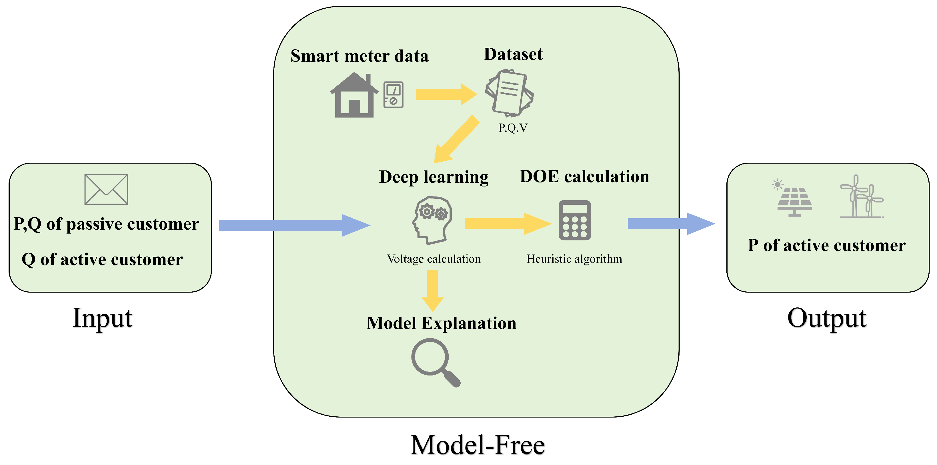
To bypass the electrical model, we propose a model-free DOE calculation approach based on deep learning and a heuristic algorithm to calculate the voltage and thus the DOEs. Once trained, this neural network can assess the voltage without requiring an electrical model. The workflow of this paper is illustrated in Figure 1. The first step involves collecting smart meter data from each user to calculate the active power $P_{i,t}$ (with injected power treated as negative), reactive power $Q_{i,t}$, and voltage magnitude $V_{i,t}$ at each bus at a given moment t. Here, $\mathrm{i}\in I=\{1,2,\dots ,C\},t\in T=\left\{t_1,t_2,\dots ,T\right\}$, where I represents the indexed set of all buses, C indicates the total number of buses, and T denotes the time indices in the dataset. This information is essential for constructing the dataset. Next, the constructed dataset is fed into a neural network model for training. The model takes the active power P and the reactive power Q as inputs, while the output is the voltage magnitude V. Through this process, the neural network learns the underlying features and topology of the network automatically. After training, the SHAP algorithm is applied to interpret the model’s results. This step explores the model’s calculations and integrates heuristic algorithms to perform DOE calculations. The algorithm is encapsulated in the model-free module, which calculates and allocates the DOEs for each active customer after inputting the active and reactive power of passive customers and the reactive power of active customers at time t.

3. Methodology

The algorithm proposed in this paper comprises three main components. First, it constructs a dataset by converting smart meter data into a format suitable for training the deep learning model. Second, the deep learning model is trained and optimized to meet the required accuracy standards. Finally, the trained model is integrated with the whale optimization algorithm to facilitate the calculation of the DOEs.

3.1. Dataset Construction

Smart meters typically provide a customer’s voltage magnitude, current magnitude, and power factor at a given time t. This information is essential for calculating the active power (with injected power set as negative), reactive power, and voltage magnitude. It is important to maintain a consistent time interval between data points, such as 15 min, 30 min, or 1 h, depending on the task. The specific data format is illustrated in Equation (1). Once the deep learning model is trained, any changes in the distribution network’s structure or line parameters necessitate dataset reconstruction and model retraining. Additionally, because the model is time-sensitive, it must be updated with new data after a certain period of use. If there is a minor loss of data in the dataset, the temporal correlation of smart meter data makes abrupt changes unlikely; therefore, the average values from the preceding and following time points are used to fill in the gaps.

$$\begin{array}{c}P=\left[\begin{array}{c}{P}_1\\ ⋮\\ P_T\end{array}\right]=\left[P_t\right]\in {\mathbb{R}}^{\left|T\right|\times \left|C\right|}\hfill \\ \\ Q=\left[\begin{array}{c}{Q}_1\\ ⋮\\ Q_T\end{array}\right]=\left[Q_t\right]\in {\mathbb{R}}^{\left|T\right|\times \left|C\right|}\hfill \\ \\ V=\left[\begin{array}{c}{V}_1\\ ⋮\\ V_T\end{array}\right]=\left[V_t\right]\in {\mathbb{R}}^{\left|T\right|\times \left|C\right|}\hfill \end{array}$$

(1)

3.2. Neural Network Generation

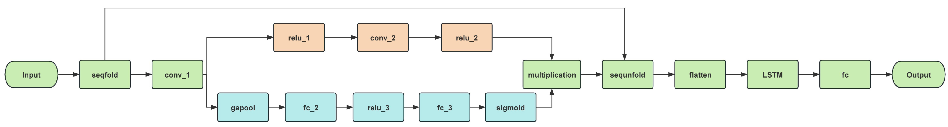
In this paper, we propose a network architecture that combines a CNN and LSTM. The CNN focuses on mapping the active power and reactive power to the voltage magnitude, while LSTM uncovers deep patterns within the voltage data sequences. This fusion enables multidimensional information extraction, thereby enhancing the model’s accuracy. However, the large scale of the distribution network and the numerous features incorporated into model training can lead to interference from irrelevant features, which impacts overall performance. Therefore, we introduce an attention mechanism to highlight important features while reducing the impact of less relevant ones, ultimately improving the model’s expressive power and generalization capability.

The model developed in this paper is illustrated in Figure 2. The CNN module in this model comprises two convolutional layers and two activation layers. The input data first pass through a 2D convolutional layer (kernel size [3, 1], 32 channels) to extract local features at each time step, followed by a $ReLU$ activation layer to enhance the network’s nonlinear capabilities. Next, a second convolutional layer (kernel size [3, 1], 64 channels) extracts deeper features, which are then processed through another $ReLU$ activation layer.

The network then incorporates a Squeeze-and-Excitation (SE) attention mechanism, constructed using a fully connected layer and a Sigmoid activation function. The SE module first reduces the feature dimensionality to 16 through a fully connected layer and then restores it to 64 dimensions using another fully connected layer. It adjusts the attention weights of the channels by generating channel-specific weights using the Sigmoid activation function. Finally, the output of the attention mechanism is multiplied element-wise with the convolutional feature map to emphasize important features and suppress less significant ones.

The features extracted by the CNN module are first passed through a sequence unfolding layer to reconstruct the sequence, restoring the convolutional features to their original sequential form. Afterward, the tiling layer flattens the high-dimensional convolutional features into one-dimensional data, making them suitable for further sequence processing. The core processing is performed by a BiLSTM layer, using bidirectional LSTMs to capture dependencies in both the forward and backward directions of the time series. The output mode is set to “last”, meaning only the hidden state of the last time step is used for the final prediction. Lastly, a fully connected layer maps the BiLSTM output to the target dimension, followed by a regression layer that produces the final output.

Once trained, the model can process input values for the active power $P_{i,t}$ and the reactive power $Q_{i,t}$ to produce the output voltage magnitude $V_{i,t}$. This approach enables voltage calculations without relying on traditional electrical modeling or tidal current analysis.

3.3. Optimizing Model Parameters

The deep learning model employed in this paper is based on a CNN-LSTM-Attention architecture. However, optimizing this model is challenging due to the numerous hyperparameters that must be set, making manual adjustments inefficient. Additionally, given the variability in distribution network structures across different regions, as well as the dynamic changes in the distribution network, periodic updates to the model are necessary. Constantly readjusting parameters during each update can be time-consuming and may hinder performance.

To streamline the model updating process, reduce parameter tuning time, and enhance model performance, we employ the WOA to optimize three key hyperparameters: the number of nodes in the hidden layer, the learning rate, and the regularization parameter. Unlike other population optimization methods, the WOA effectively balances global exploration and local exploitation by mimicking the natural behavior of humpback whales as they trap prey using bubble nets.

The WOA simulates the humpback whale’s unique foraging approach, which consists of three main phases: seeking prey, bubble net feeding, and searching for food. In this context, each whale’s position represents a potential solution, with the global optimal solution achieved through continual updates of whales’ positions in the solution space. For the parameter optimization task, the WOA is initialized by setting zero vectors as the position vectors for potential solutions, with the fitness score of the optimal solution initialized to positive infinity. The optimization objective is to minimize the root mean square error (RMSE). During the iterative process, the position of the leading whale is regularly updated. Each search agent compares its fitness to the current global optimal solution to determine whether to update the leader. If a search agent’s fitness exceeds the current optimal solution, the solution and its position are updated. The positions of all search agents are continuously adjusted based on variables (A, C, b, l, p), which are calculated from random numbers $r_1$ and $r_2$. Here, A controls the search agent’s step size within the range [−1, 1], C regulates the moving direction within the range [0, 2], and b is a positive value that controls speed. The variable l determines the movement distance, set randomly within the range [−1, 1]. If $p<0.5$, the agent follows the leader or explores randomly, whereas $p>0.5$ activates a local search update, adjusting positions based on proximity to the leader and the parameters b and l. This iterative process continues until the optimal hyperparameters are identified. Its iterative update rule is as follows:

$$X(t+1)=\left\{\begin{array}{c}{X}^{*}\left(t\right)-A·D,p\le 0.5\\ D^{\prime }\times {\mathrm{e}}^{bI}\times cos\left(2\pi I\right)+X^{*}\left(t\right),p>0.5\end{array}\right.$$

(2)

3.4. DOE Allocation with WOA

Consequently, calculating the DOEs involves determining the maximum allowed injected power at each bus while accounting for distribution grid constraints. This paper focuses on triple-balanced grids, where the primary constraint is the voltage limit, as expressed in Equation (3):

$$V_{i,t}<{1.05V}_0$$

(3)

$V_{i,t}$ represents the voltage magnitude at bus i at the specified time t, and $V_0$ is the voltage at the root bus. The objective function aims to maximize the DOEs, which translates to maximizing the sum of the injected power for each active customer. Since the active power is treated as negative when defining the injected power, the objective function is formulated as follows:

$${\displaystyle f\left(x\right)=min\sum _{j\in J}{P}_{j,t}^a}$$

(4)

where $P_{j,t}^a$ denotes the active power injected by the active customers, $J\in j=\{1,2,\dots ,C_a\}$ represents the set of active customers, $C_a$ is the total number of active customers, and t encompasses the time indices in the dataset $\mathrm{t}\in T=\{1,2,\dots ,T\}$. It is important to note that the calculations for the power export and import limits are symmetric; therefore, this paper focuses solely on the power export limit, omitting a separate discussion of power import limits.

This paper employs the WOA to calculate DOEs, and the calculation steps are outlined as follows:

• Initialization: Set the active power of each active customer to zero (i.e., $p_{j,t}^a=0$). Using the trained model, calculate each bus’s voltage $V_{i,t}$. If the voltage meets the constraints, this configuration is designated as the optimal solution, and the optimal fitness value $f_{opt}\left(x\right)$ is calculated.
• Optimization Search: Utilize the WOA to search for the optimal $p_{j,t}^a$. After each search iteration, apply the trained model to verify whether the constraints are satisfied. If the constraints are not met, assign a fitness value of infinity; otherwise, calculate the fitness value normally.
• Determination: Compare the fitness value from the current iteration with the optimal fitness value. If the current fitness is better, update the solution to reflect this new optimal solution and replace the fitness value, then return to step 2. If not, proceed directly to step 2.
• End Condition: The calculation concludes when the maximum number of iterations is reached or when a stopping criterion is satisfied.

Upon completion of these calculations, the optimal active power for each active customer at time t is obtained. The DOE is defined as

$$P_{j,t}^{DOE}=-P_{j,t}^a$$

(5)

The injected power of the jth active customer at time t must satisfy $p_{j,t}^{in}\le P_{j,t}^{DOEs}$, ensuring that the voltage in the distribution network remains within acceptable limits.

4. Case Study

This paper constructs a dataset using simulation data from the IEEE 33−bus distribution network model. The dataset includes the active power, reactive power, and voltage magnitude for each bus, with the root bus voltage set at 12.66 kV. In addition, the photovoltaic penetration rate is assumed to be 100%, i.e., each bus may inject power into the grid, and each bus may have positive and negative active power.

4.1. Training Models

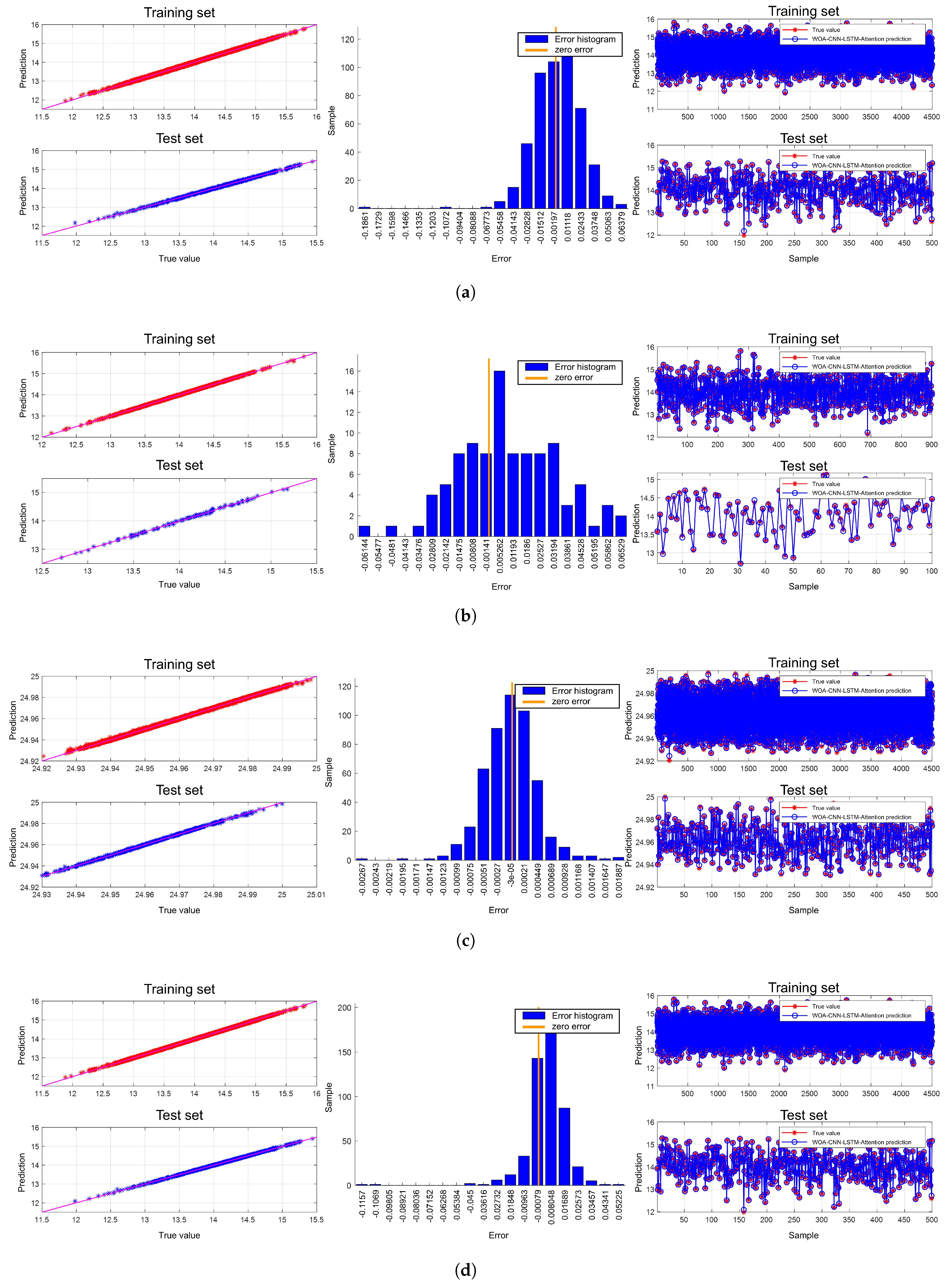
The model presented in this paper utilizes 65 input features, including the active and reactive power along with the root bus voltage, to predict 32 output voltages. The initial training set consisted of 5000 data points, divided into 90% for training and 10% for testing. On the training set, the model achieved an $R^2$ of 0.9995, a mean absolute error (MAE) of 0.0068 kV, and a mean absolute percentage error (MAPE) of 0.049%. For the test set, the $R^2$ was 0.9993, with an MAE of 0.0064 kV and an MAPE of 0.053%. The output voltages for bus 33 were analyzed to validate the model’s predictions, as illustrated in Figure 3a. The results demonstrate a high level of accuracy, with most sample points lying along the 45° line and absolute errors primarily below 0.015 kV, while nearly all are under 0.05 kV. The fitting curve further confirms that the model accurately predicted single-point outputs and effectively captured the overall trend of voltage changes.

Recognizing that the distribution network structure may evolve, the model was also tested with a reduced training set of 1000 data points to assess its performance with less data. Notably, the model parameters remained unchanged during this retraining. After reducing the dataset, the test set yielded an average $R^2$ of 0.9982, an MAE of 0.0131 kV, and an MAPE of 0.082%. Although there was a slight decrease in accuracy, the prediction performance remained commendable. The results for bus 33, as shown in Figure 3b, further illustrate that the model maintained satisfactory predictive performance, with sample points still clustering around the 45° line. Although the error histogram appears more scattered and the maximum absolute error increased to 0.06 kV, the model continued to fit the voltage curves accurately.

An additional experiment was conducted using the IEEE 14−bus distribution network model to explore the model’s applicability across varying distribution network structures. It is important to note that when replacing the dataset and the grid model, the deep learning model did not change any parameters but relied on the whale optimization algorithm to tune the parameters automatically. After replacing the distribution grid model, the average $R^2$ of all model outputs on the test set was 0.9994, the MAE was 0.0001 kV, and the MAPE was 0.0005%. After replacing the distribution network model, the model increased rather than decreased its prediction accuracy, reflecting the superior adaptivity of the model. In the case of bus 14, the specific output of the model is shown in Figure 3c, and it can be seen that the model has a superior fitting and that most of the absolute errors do not exceed 0.0005 kV.

To evaluate the performance of the proposed method under varying DER environments, we adjusted the photovoltaic penetration rate from 100% to 50%, meaning only half of the buses could inject power into the grid. The model was retrained without altering its parameters. After retraining, the test set achieved an average $R^2$ of 0.9990, an MAE of 0.0081 kV, and an MAPE of 0.056%. The detailed results, as illustrated in Figure 3d, indicate that the model continued to perform exceptionally well on both the training and test sets. Most errors remained within a narrow range of 0.009 kV, demonstrating the model’s ability to adapt effectively to different DER environments while maintaining high computational accuracy. This highlights the model’s strong scalability and robustness.

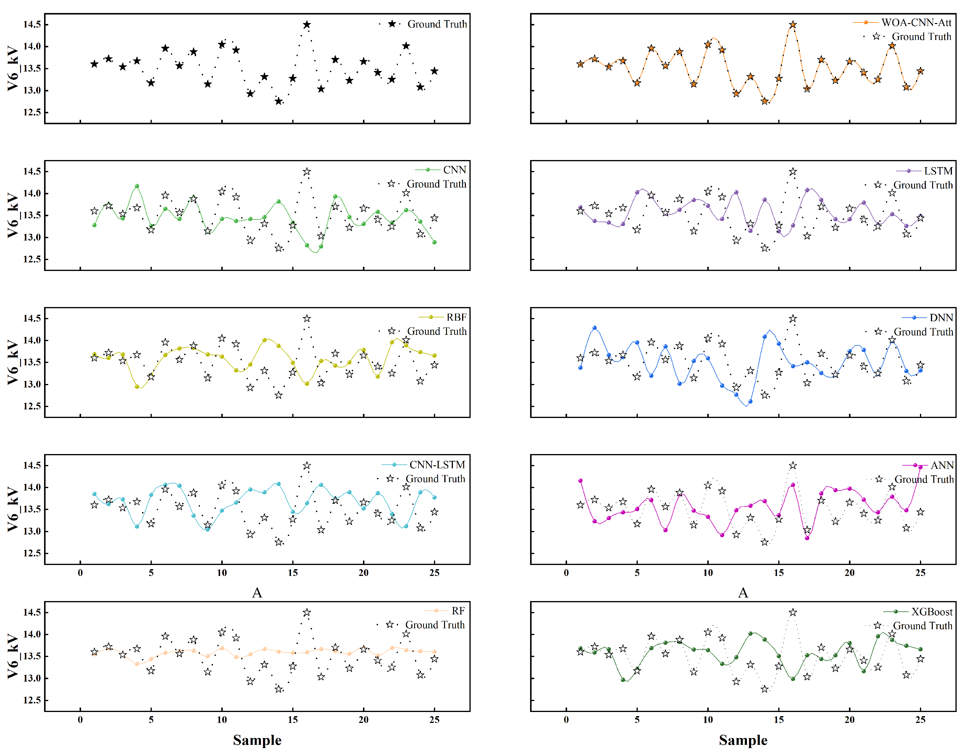
In addition, to demonstrate the superior performance of the proposed model, this paper selected other commonly used models for training, including commonly used deep learning models and powerful machine learning algorithms, such as random forest and XGBoost, with the training results summarized in

Table 1. Performance metrics of different deep learning models.

	RMSE (kV)	MAE (kV)	MAPE (%)
CNN	1.1418	0.7458	5.2841
LSTM	0.1819	0.1408	1.0491
RBF	0.0281	0.0199	0.1438
DNN	0.0881	0.0706	0.5119
CNN-LSTM	0.0589	0.0442	0.3190
ANN	0.0378	0.0295	0.2115
RF	0.2843	0.2131	1.471
XGBoost	0.0603	0.0461	1.5776
WOA-CNN-LSTM-Att	0.0116	0.0074	0.0537

. The model presented here outperformed the other models in terms of training accuracy and fitting effect, with its RMSE, MAE, and MAPE being approximately one-third of those of the second-ranked deep learning model, RBF. Furthermore, compared to the unoptimized CNN-LSTM model, the optimizations applied in this paper reduced the metrics to about one-sixth of their original values. Figure 4 illustrates the predictions of different models for the voltage and their fitting effects on the voltage curve. Evidently, the model constructed in this paper achieved high accuracy in predicting the voltage and effectively captured its dynamic changes. Unlike the other models, the proposed model consistently provided accurate predictions for each sample point, aligning closely with the original data’s variation. In summary, the deep learning model developed in this paper demonstrates superior prediction accuracy and fitting performance compared to the alternative methods.

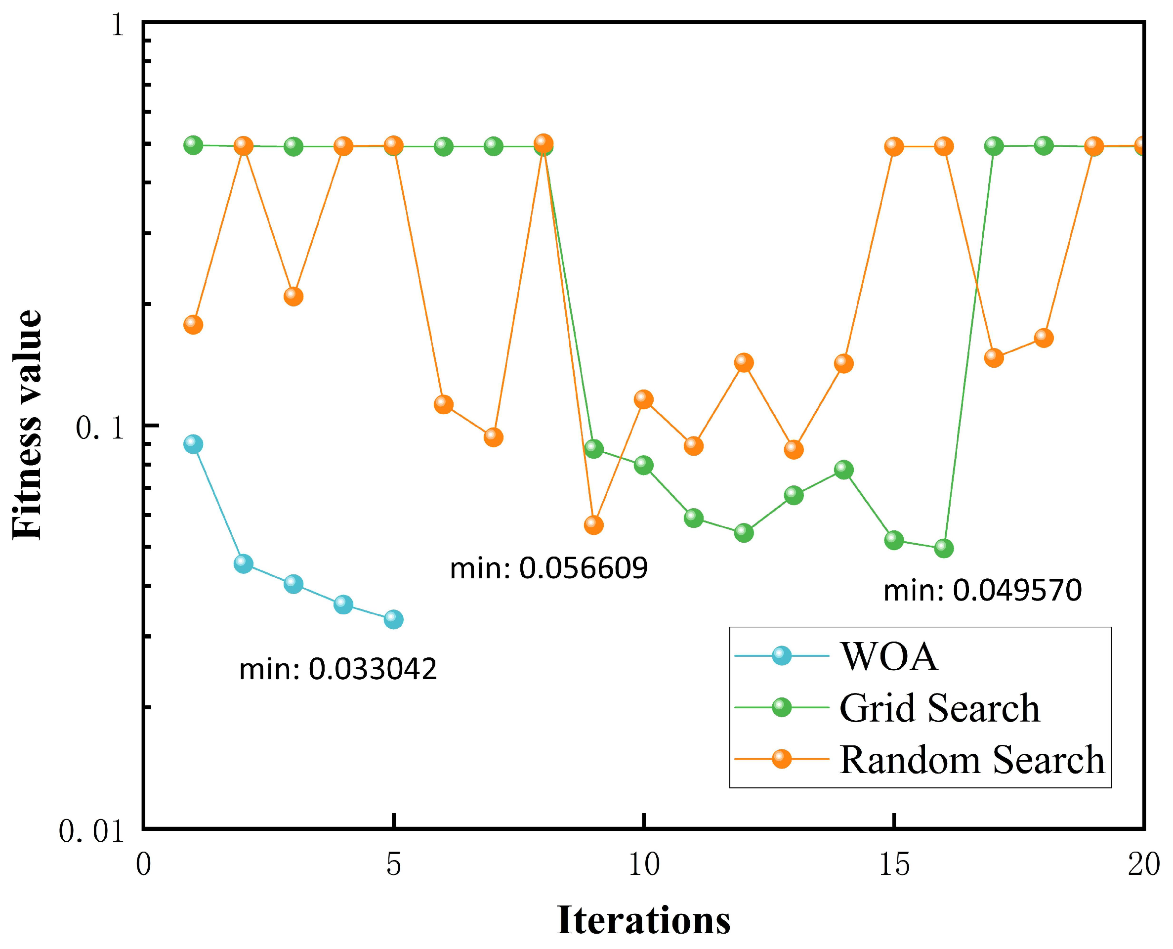
This paper further highlights the advantages of the WOA for parameter optimization by comparing it to commonly used tuning methods, such as grid search and random search. The optimization process used the mean squared error (MSE) as the fitness function, with the maximum number of epochs set to 20 to speed up the optimization. The results, as shown in Figure 5, reveal that the WOA algorithm achieved the lowest fitness value of 0.033042 after just five iterations, outperforming both grid search and random search, which were less effective even after 20 iterations. Additionally, the WOA’s optimization curve decreases monotonically, indicating a consistent improvement in model performance. This suggests that, when necessary, increasing the number of iterations can continue to refine the model. In contrast, the curves for grid search and random search exhibit significant randomness, indicating that increasing the number of optimization attempts does not necessarily lead to better results. This unpredictability can complicate the optimization process in practice. In conclusion, the WOA not only improves model performance but also enhances the efficiency of the optimization process, making it a more reliable and practical choice than traditional methods.

4.2. Uncovering Deep Learning Models

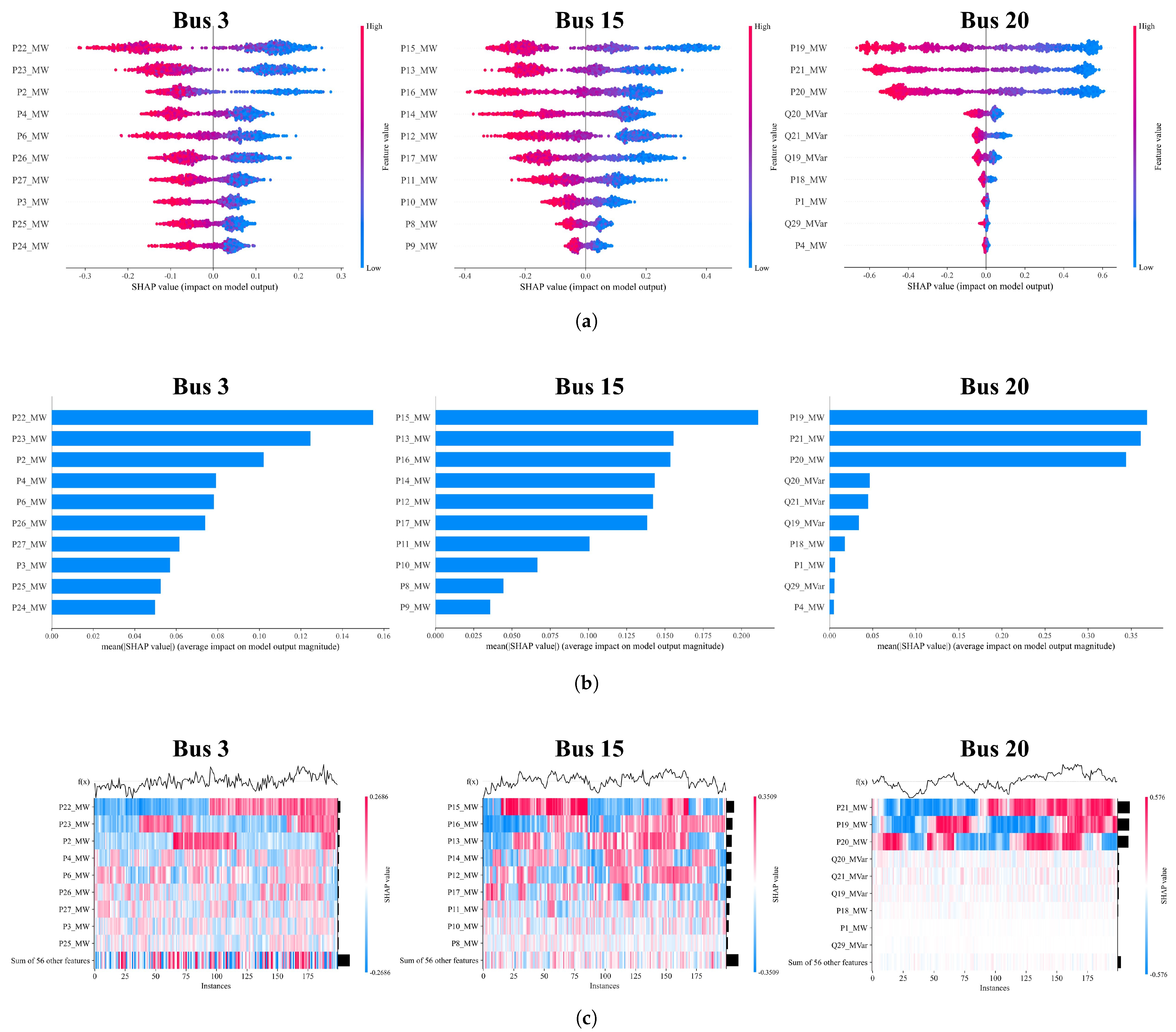
Due to the black-box nature of deep learning models, understanding their internal workings can be challenging, complicating their application in practical engineering. This paper employs the SHAP algorithm to highlight the model’s operations and learning dynamics, addressing this issue. The SHAP algorithm, grounded in game theory, interprets machine learning models by treating all features as “contributors”. For each prediction, the model generates a prediction value, and the SHAP value reflects the contribution of each feature to that prediction. This algorithm assesses the importance of individual features and elucidates how each feature influences the output.

In this paper, buses 3, 15, and 20 serve as examples to illustrate how the SHAP algorithm helps explain the model’s calculations of their voltages and the influence of other buses on these voltages. Figure 6a illustrates the impact of each feature on the bus voltages. The left axis identifies the top ten features ranked by importance, while the bottom axis displays the corresponding SHAP values. Each point on the graph represents a sample, with red points indicating higher feature values and blue points indicating lower values. The distribution of sample points reveals that for buses 3, 15, and 20, red points are primarily found on the left, while blue points are on the right. This pattern suggests that a higher active power from other buses correlates with a lower voltage at the target bus. Conversely, as the active power from other buses decreases, the voltage at the target bus tends to increase, aligning with established physical principles. Taking bus 3 as an example, the SHAP summary plot illustrates how the active power at bus 22 impacts the voltage at bus 3 within a range of approximately −0.3 kV to 0.3 kV. Blue data points represent lower active power levels, indicating power injection into the grid. Depending on the magnitude of the injected power, the voltage at bus 3 can increase by up to 0.3 kV. Conversely, if bus 22 transitions from injecting low power (purple data points) to absorbing power from the grid (red data points), the voltage at bus 3 may decrease by approximately 0.4 kV. This shift highlights the sensitivity of bus 3’s voltage to changes in the active power at bus 22. In practical applications, the SHAP algorithm provides valuable insights for controlling the influence of the active power at one bus on the voltage magnitude of other buses. By understanding these relationships, operators can determine effective regulation ranges to maintain network stability.

Figure 6b presents histograms depicting the feature importance for buses 3, 5, and 20. For bus 3, the primary factors influencing its voltage magnitude are the active power at buses 22, 23, and 2, with similar importance levels among these features. This indicates that bus 3 is connected to multiple branches, meaning its voltage is affected by the interactions within the entire distribution network. Consequently, any change in a distant bus can lead to voltage fluctuations at bus 3. For bus 15, the most significant influences come from its adjacent buses, with its active power being the most critical factor. This highlights that, as a central bus in the distribution network, bus 15’s voltage is predominantly shaped by itself and its neighboring buses, although other features also play a noteworthy role. In the case of bus 20, the active powers at buses 19, 21, and itself are particularly crucial for its voltage magnitude, surpassing the importance of other features. This suggests that, as the end bus of the distribution network, bus 20’s voltage is primarily determined by its state and the conditions of nearby buses, in contrast to the influences seen at buses 3 and 15. Similarly, using bus 3 as an example, the SHAP feature importance histogram reveals that the active power at bus 22, bus 23, and bus 2 has the most significant impact on its voltage level. Consequently, if bus 3’s voltage is nearing an overrun and requires prompt and cost-effective mitigation, adjusting the active power injections at these three buses should be prioritized to stabilize the voltage. In practical applications, the SHAP algorithm provides valuable insights by analyzing the correlation between bus voltages and the characteristics of other buses. This enables operators to identify and prioritize effective adjustment targets, ensuring efficient voltage regulation within the network.

Figure 6c presents a heatmap illustrating the influence of each feature on the bus voltages. The color intensity reflects the magnitude of each feature value, and the transparency indicates the degree to which each feature affects the voltage magnitude at each bus. The black bar on the right side highlights the contribution of each feature to the corresponding voltage magnitude. For bus 3, the contributions from various features are relatively similar, suggesting that all features, aside from the most important ones, play a role in determining its voltage. This finding underscores the interconnected nature of the distribution network, where the voltage at bus 3, a critical junction, is influenced by the overall operation of the network. The voltage at bus 15, serving as a central point in the network, is predominantly influenced by its neighboring buses, although other, more distant buses also exert some effect. In contrast, the voltage at bus 20 primarily depends on the conditions of the nearby buses along the same branch. As the terminal bus of the distribution network, local factors significantly influence its voltage. Using bus 3 as an example, the SHAP heatmap indicates that the influence of each feature on its voltage magnitude is relatively uniform. As a result, achieving a wide-range regulation of bus 3’s voltage by adjusting the active and reactive power of only a few buses may not be sufficient. Instead, it may require coordinated regulation across multiple buses to reach the desired voltage level. In contrast, for bus 22, the active power at bus 19, bus 20, and bus 21 has a dominant impact on its voltage magnitude. This means that the voltage at bus 22 can typically be regulated by adjusting the active power at these three buses alone. The SHAP algorithm provides valuable insights by quantifying the influence of each feature on the bus voltage. This enables the formulation of targeted and effective strategies for voltage regulation at specific buses, enhancing operational efficiency and control.

Through SHAP analysis, this paper clarifies how different features affect bus voltages and identifies the primary dependencies for each bus’s voltage magnitude in the deep learning model, enhancing interpretability. Furthermore, when specific bus voltages exceed safe limits, the insights from SHAP analysis can guide targeted adjustments at specific buses, thereby ensuring the overall safety of the distribution network.

4.3. DOE Allocation

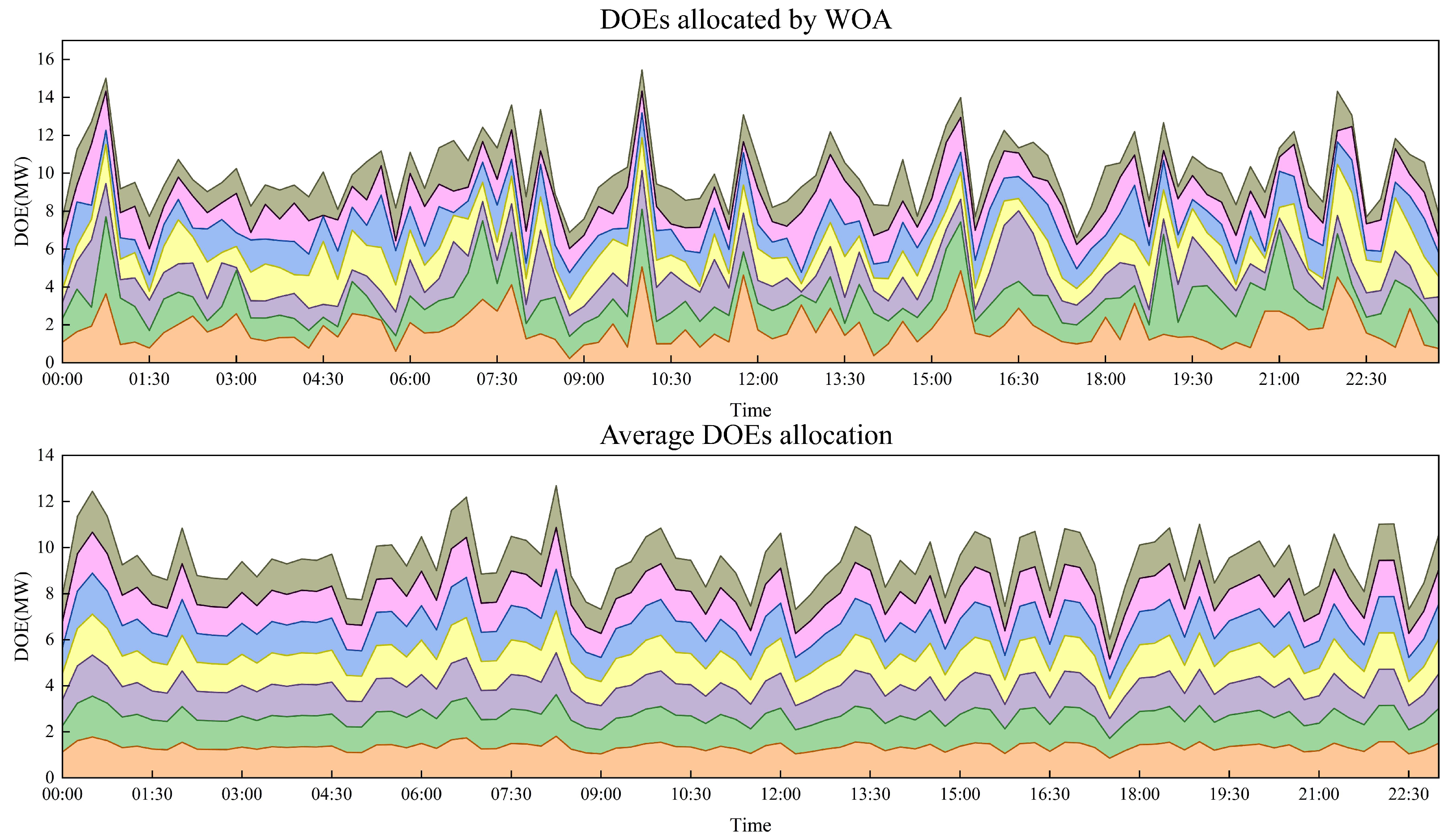
After establishing the deep learning model, we calculated the DOEs using two methods: the WOA and equal allocation. The objective function focused on maximizing the injection power while considering voltage constraints. To simulate real-world conditions, we assumed a photovoltaic penetration rate of 20%. The results are illustrated in Figure 7, where each color block represents the assigned DOEs for an active customer, reflecting its upper limit on the injection power. The DOE curve generated by the WOA exhibited rapid fluctuations, in contrast to the relatively flat curve of the equal distribution method. This disparity can be attributed to the WOA’s global optimization capabilities and randomness, which allowed it to identify optimal solutions independently at various times. Consequently, the WOA was more effective at uncovering potential optimal solutions than the equal allocation method. Moreover, the DOE trends for each active customer derived from the WOA were mainly consistent, suggesting that the available DOEs were primarily influenced by the overall operating conditions of the power grid. Additionally, the similar sizes of the DOE color blocks for each active customer at the same time point indicate that simultaneously increasing the maximum injectable power at each bus could lead to a higher total maximum injectable power for the system.

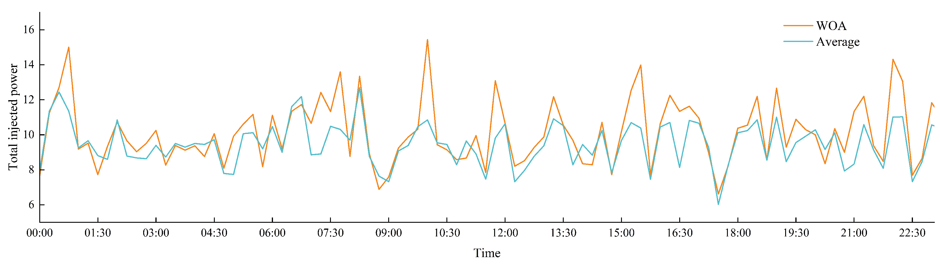
To evaluate the effectiveness of the WOA, we compared the total DOE values obtained at each time point using both the WOA and equal allocation methods, as illustrated in Figure 8. The results indicate that the total DOEs calculated with the WOA were consistently higher than those derived from the equal allocation method, often significantly so at various time points. This enhanced performance can be attributed to the WOA’s ability to identify potential optimal solutions more effectively than the equal allocation method, resulting in a greater total capacity for the injection power. However, there were a few time points where the total DOEs from the WOA were slightly lower than those from the equal allocation method. This discrepancy can be linked to the inherent randomness of the WOA, which could be addressed by increasing the number of iterations. Overall, the findings confirm that the WOA yields a higher total number of DOEs than the equal allocation method, highlighting its superior optimization capabilities.

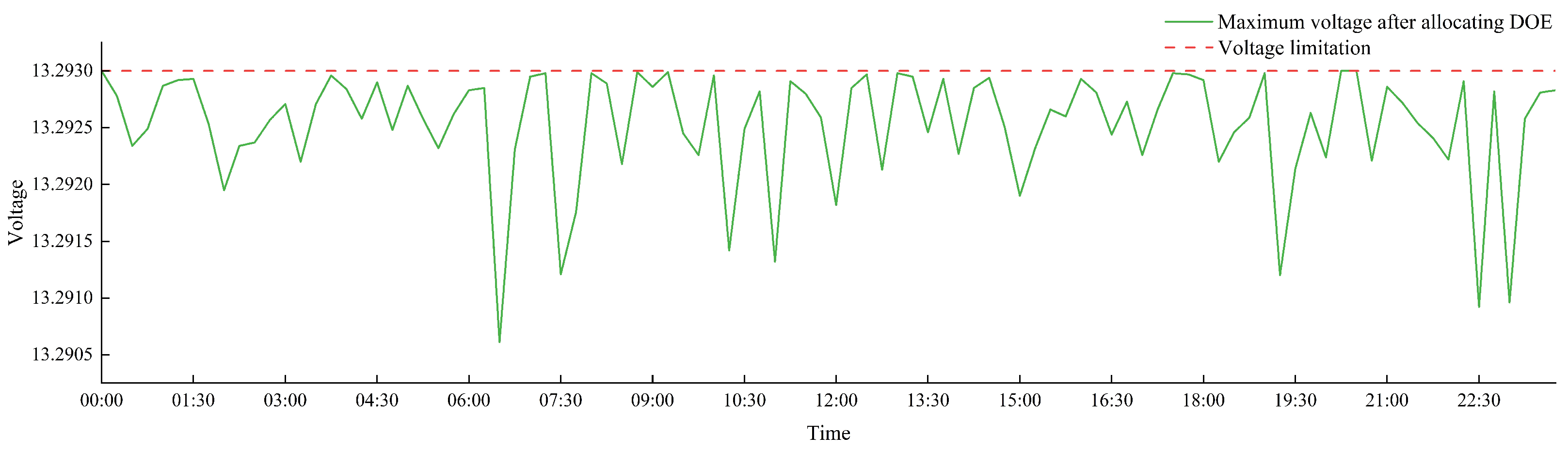
To assess the feasibility of the WOA, we recalculated the voltage at each bus using the derived DOEs and identified the maximum voltage values to ensure compliance with the voltage limits. The results, as presented in Figure 9, demonstrate that under the WOA calculations, no bus exceeded the voltage limits. The available voltage capacity was primarily optimized, thus enhancing energy utilization while ensuring the safe operation of the distribution network.

5. Conclusions

Power distribution companies often face challenges in accurately calculating DOEs due to difficulties obtaining reliable electrical models of their distribution networks, which complicates power-flow calculations. This paper addresses this issue by employing a deep learning model to effectively capture the topology of the distribution network, thereby eliminating the need for traditional power-flow calculations. Additionally, we integrate the WOA and an attention mechanism to enhance the model’s accuracy, operational efficiency, and adaptability. The SHAP algorithm is also utilized to interpret the model, facilitating its practical application. Ultimately, the proposed approach is validated through simulations on an IEEE 33−bus distribution network model, demonstrating significant improvements in results.