Modeling and Analysis of Current-Carrying Coils Versus Rotating Magnet Transmitters for Low-Frequency Electrodynamic Wireless Power Transmission

Abstract

Current-carrying coils and rotating permanent magnets can be used to create time-varying excitation magnetic fields for electrodynamic wireless power transmission (EWPT). Both types of transmitters produce low-frequency, time-varying fields at the locations of the receiver, but with fundamental differences. A coil transmitter produces a uniaxial magnetic field, where the direction of the field is along a single axis, but the amplitude varies in a bipolar fashion. In contrast, a rotating magnet transmitter produces a rotating magnetic field, with the amplitude varying in two orthogonal directions. Building on prior work for coil transmitters, this manuscript presents the modeling and a simulation framework for rotating magnet transmitters. The performance of an EWPT system is then studied both theoretically and experimentally for both transmitter types. For the same B-field amplitude (501 µT) and a fixed transmitter-receiver distance of 12 cm, a receiver driven by a coil transmitter produces 38 mW, whereas the same receiver driven by a rotating magnet transmitter produces 149 mW, nearly four times higher. This power increase is a result of 50% higher receiver rotation speeds using the rotating magnet transmitter. The power transfer efficiency is also six times higher for the rotating magnet transmitter.

1. Introduction

Wireless Power Transfer (WPT) offers the potential to supply electrical energy from a transmitter to a receiver without physical connections. While most recent advances in WPT have been directed towards EV charging, primarily focusing on inductive power transfer (IPT) and resonant inductive power transfer (RIPT) systems, as summarized in [1], there remain application spaces where low-frequency, mechanically driven systems like rotating magnet transmitters offer distinct advantages. In particular, rotating magnet WPT systems can provide mid-range field penetration in environments where high-frequency fields are heavily attenuated due to moisture, such as underground in precision agriculture. Given that active research and commercialization efforts in rotating magnet WPT systems [2] ceased recently, revisiting this approach under modern application requirements where the state-of-the-art resonant inductive systems fall short, provides a valuable opportunity to re-evaluate its potential. Compared to the more common inductively coupled WPT solutions, electrodynamic wireless power transfer (EWPT) sets itself apart by employing a mechanically responsive permanent magnet in the transmitter and/or receiver. EWPT offers distinct advantages, particularly in its ability to transfer energy over greater distances and generally at lower electrical frequencies, which is important for minimizing unwanted interference with objects situated between the transmitter and the receiver. Furthermore, the power transfer capacity for inductive WPT scales with the surface area of the receiver coil, whereas the power capacity of an EWPT receiver depends on the volume of the receiver magnet [3]. Consequently, EWPT offers distinct size advantages for use cases where the receiver has a limited surface area (such as compact sensor nodes, wearable electronics, medical implants, etc.) [4,5].

In EWPT, the receiver magnet can be mechanically supported in multiple ways to capitalize on the forces and torques acting on it. For example, torsional forces on the magnet can cause an oscillation/vibration (generally at a mechanical resonant frequency) [6] or can allow the magnet to continuously rotate [2]. Compared to oscillating magnet receivers, fully rotating magnet receivers generally produce a higher power output [7] mainly due to the 360-degree displacement offered by rotating magnet receivers, compared to the low displacement generally seen in resonant vibrating magnet receivers. This work focuses solely on the modeling and analysis of rotating magnet receivers.

To excite the physical rotation of rotating magnet receivers, both current-carrying coil transmitters and rotating permanent magnet transmitters have been utilized, as shown in Figure 1a–c. Figure 1d–g illustrates the fabrication of the receiver. The EWPT receiver explored in this case is an off-the-shelf, commercially available coreless DC motor that was modified into a receiver by replacing the ferromagnetic stainless-steel housing with a 3D printed shell made of PLA (Poly Lactic Acid). A custom 3D-printed base was used to access all five electrical nodes.

Coil-based transmitters typically employ conductive windings of multiple turns to produce a time-varying magnetic field. In contrast, rotating magnet transmitters generally employ a permanent magnet driven by a DC motor to produce a time-varying field. Rotating magnet transmitters have been observed to yield higher power output and higher power transfer efficiency [2,8,9], most commonly attributed to the fact that the magnet produces a large magnetic field without any power sources. Achieving similar magnetic field strengths with current-carrying coils requires large currents and hence significant resistive losses in the coil windings (assuming the coil is not superconducting). The only power penalty for a rotating magnet transmitter is the power required to mechanically rotate the magnet, which can be quite low if an efficient drive motor and low-loss bearings are used. Additionally, a coil tends to be flat in geometry but large in diameter, contrary to a rotating magnet that tends to be compact, but in volume. Compared to the coil transmitter, the rotating magnet transmitter can generate noise and vibration at higher frequencies. Special care needs to be taken when designing the bearing for the rotating magnet transmitter. Another interesting observation is that the permanent magnet creates a strong DC field (and field gradients) that cannot be controlled. When not in motion, the rotating magnet transmitter can attract small metallic objects, creating a hazard.

In addition to these physical differences between the transmitter types, there is another fundamental difference in the magnetic fields that are produced. Coil transmitters and rotating magnet transmitters both produce time-varying magnetic fields, but those fields differ significantly in amplitude and orientation at the location of the receiver. At the receiver’s position, the magnetic field produced by a coil is uniaxial (oriented in a specific axis), with the magnitude of the magnetic field oscillating between both positive and negative values along the axis. Figure 2a–e exhibits this variation in magnitude of the uniaxial field from the coil transmitter. In contrast, the magnetic field produced by the rotating magnet transmitter is more complex. It changes in amplitude and direction and never passes through a zero-field condition. Figure 2f–j illustrates this variation in magnitude and orientation of the B-field vector generated by the rotating magnet transmitter at the location of the receiver, located relatively far from each other. Interestingly, notice that as the magnet in the transmitter rotates in a clockwise pattern, the B-field vector at the position of the receiver rotates in the opposite direction, i.e., counterclockwise. The amplitude of the counter-rotating magnetic field also varies, i.e., from a maximum of $B_0$ to a minimum of $B_0/2$. This complexity in the rotating magnetic field has a significant impact on the performance of the EWPT receiver.

In this paper, we present a modeling approach to simulate EWPT using a rotating magnet receiver, driven either by a pancake-shaped coil transmitter or a rotating magnet transmitter that produced a uniaxial field and a biaxial field, respectively. The receiver used here is a previously developed EWPT rotating magnet receiver [10]. The remainder of this paper is organized as follows: Section 2 discusses methods and materials. Section 3 introduces the analytical modeling and simulation of the EWPT system with each transmitter type, and, in particular, the angular velocity behavior of the rotating magnet receiver in three distinct regions: random oscillation, ramp-up, and steady-state rotation. Section 4 provides experimental results of the receiver driven separately by the two types of transmitters and compares those results to the model simulations, and discusses some observations from the simulation, experimental and analytical results. Section 5 concludes this discussion.

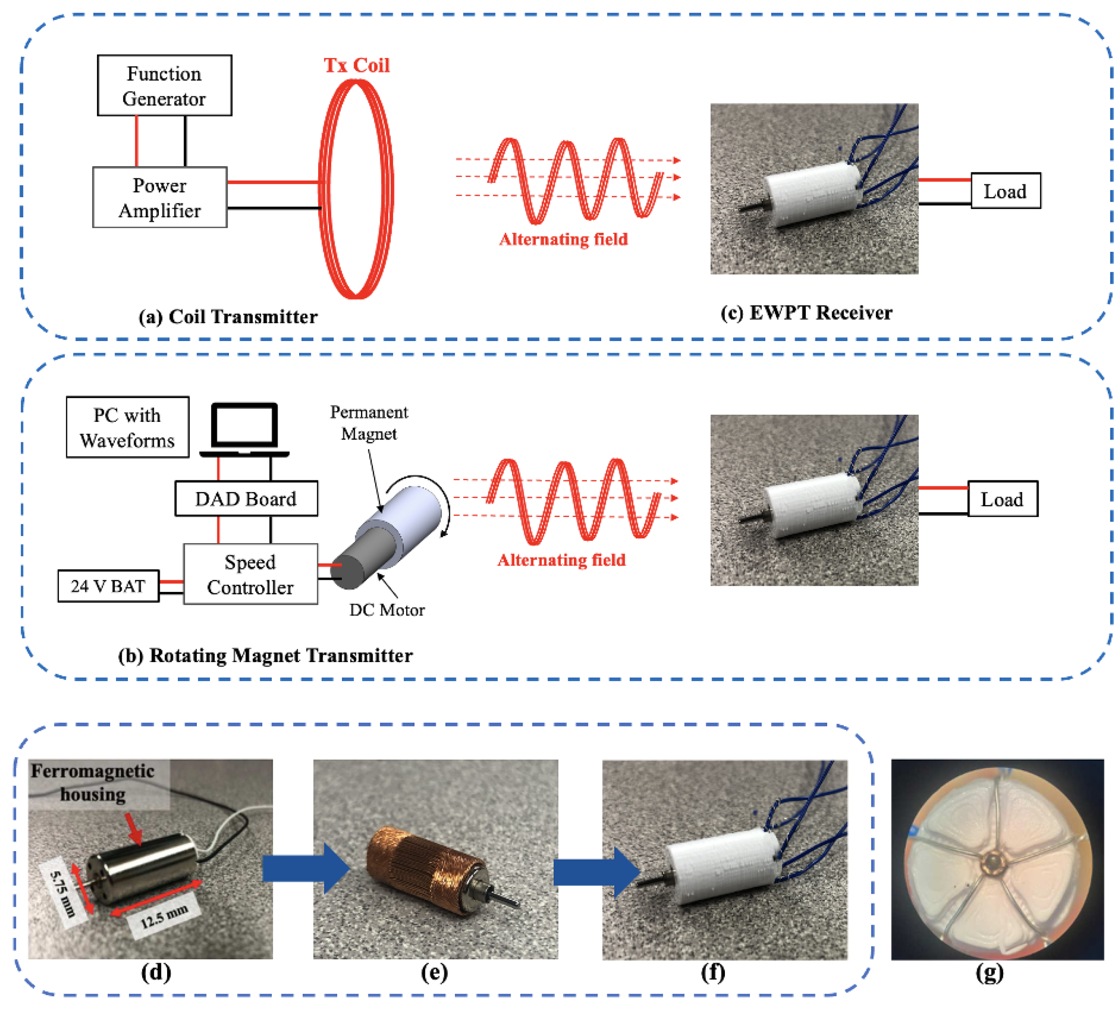
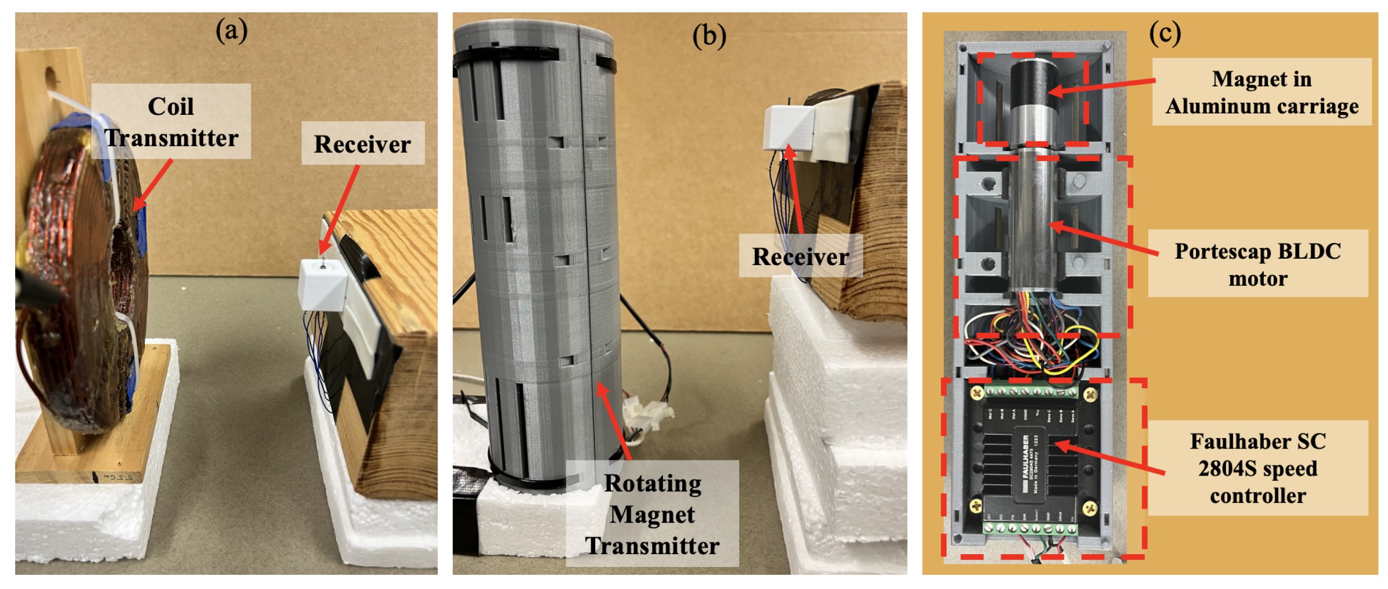
2. Methods and Materials

The experimental setup consists of a rotating magnet receiver driven either by a coil-based transmitter or a rotating magnet transmitter as shown in Figure 3a and Figure 3b, respectively. The rotating magnet receiver is a custom-modified, commercial off-the-shelf, five-phase DC motor (RC Geek 8520 done coreless motor). The ferromagnetic stainless-steel housing of the motor is replaced with a non-magnetic 3D printed housing, and a custom connector is used to make electrical connections to all five phase windings [10]. A simple, single resistor is used as a load, connected across terminals 1 and 3 of the five-winding phases.

The coil-based transmitter is a pancake-shaped coil comprising 169 turns of 16 AWG (American Wire Gauge) copper wire, with an outer diameter of 15 cm, an inner diameter of 5.75 cm and a thickness of 1.6 cm. The inductance and the resistance of the coil are 3 mH and 0.8 Ω, respectively. For the coil-based transmitter, an AC waveform is generated by an Agilent signal generator (33120A), which is amplified using a Crown XLS2500 current amplifier. The current from the amplifier is further fed into the coil transmitter. The coil produces a time-varying magnetic field, and the frequency is swept from as low as 1 Hz up to the pull-out frequency with a ramp rate of 5 Hz/s. The input current into the coil is measured using a TCP312A current probe connected to a TCPA300 current probe amplifier. Input voltage into the coil is measured using a Teledyne Lecroy AP-031 differential probe.

Alternatively, the rotating magnet transmitter, as shown in Figure 3c, comprises a center-bored, cylindrical magnet (K&J Magnetics RA2ADIA; OD = 1.59 cm, ID = 0.32 cm, length = 1.59 cm) that is magnetized perpendicular to the cylinder axis, mounted on a Portescap slotless brushless DC (BLDC) motor (22ECS60) driven by a Faulhaber SC-2804S-4475 speed controller. The motor is programmed using a Digilent Analog Discovery-2 board with a custom script on Waveforms software v3.21.3 (Digilent) that sweeps the duty cycle of the PWM signal of the input voltage to the BLDC motor and produces a rotating magnetic field. The motor requires a 24V DC source, which is applied using an Agilent E 3630A DC power supply. A Lakeshore transverse Gauss probe (HMNT-4E04-VR) connected to a Lakeshore 475DSP Gaussmeter is used to measure the field amplitudes produced from the transmitters.

The frequency of the time-varying AC field is varied from 1 Hz up to a steady-state condition where the receiver magnet is rotating stably. Figure 4 shows an example of the measured voltage across the load resistor as a function of frequency. The output voltage is linked to the motion of the receiver magnet. While Figure 4a captures the whole sweep from 1 Hz to 135 Hz, Figure 4b illustrates the magnet motion causing it to randomly oscillate. As the frequency is swept further, the randomly oscillating magnet locks with the frequency of the magnetic field, similar to a synchronous generator, and continuously rotates. This rotation induces a sinusoidal voltage in the windings as seen in Figure 4c and delivers current and power across the load. At a particular frequency, the receiver loses its synchronization with the magnetic field and stops spinning. The frequency at which the magnet loses its synchronization is called the ’pull-out’ frequency, analogous to the pull-out torque in a synchronous generator.

The pull-out frequency depends on the total damping in the system, which includes both viscous mechanical damping (bearing loss and windage) and load-dependent electromechanical damping. The electromechanical damping is higher at lower resistive loads $R_L$, (e.g., around 1 Ω), where large currents flow through the winding, generating a strong opposing torque that reduces the pull-out frequency. As the resistive load increases (e.g., up to 10,000 Ω), the current flowing in the surrounding pick-up windings decreases, leading to a weaker opposing torque and correspondingly higher pull-out frequencies. In the open-circuit condition, $(R_L\to \infty )$, where no current flows, the pull-out frequency typically reaches its maximum value.

3. Modeling and Simulation

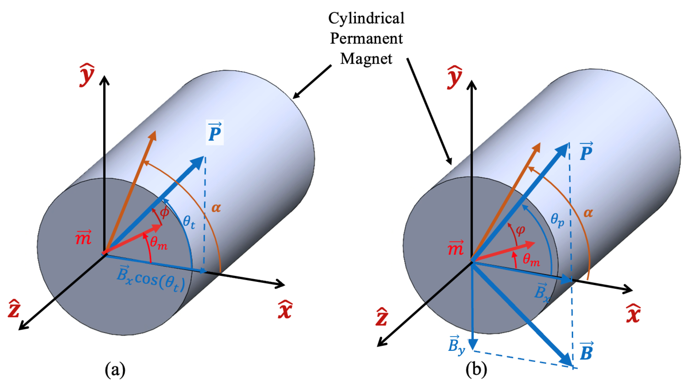
In this section, the basic relationships between the magnetic field, magnetic moment, induced torque, and electrodynamic transduction coefficient are described, resulting in a steady-state equation of motion for the receiver magnet and the instantaneous power across the load resistor. The analytical solution is found for both cases with and without electrical load, for the synchronous mode of operation, from which the pull-out frequency is determined. MATLAB and Simulink (v. R2021b) are used to solve the second-order equations. First, the equations for the coil transmitter (uniaxial) are briefly discussed, followed by a detailed discussion on the rotating magnet transmitter (biaxial). The detailed analysis of the receiver driven by the coil transmitter is given in [11].

3.1. Theory

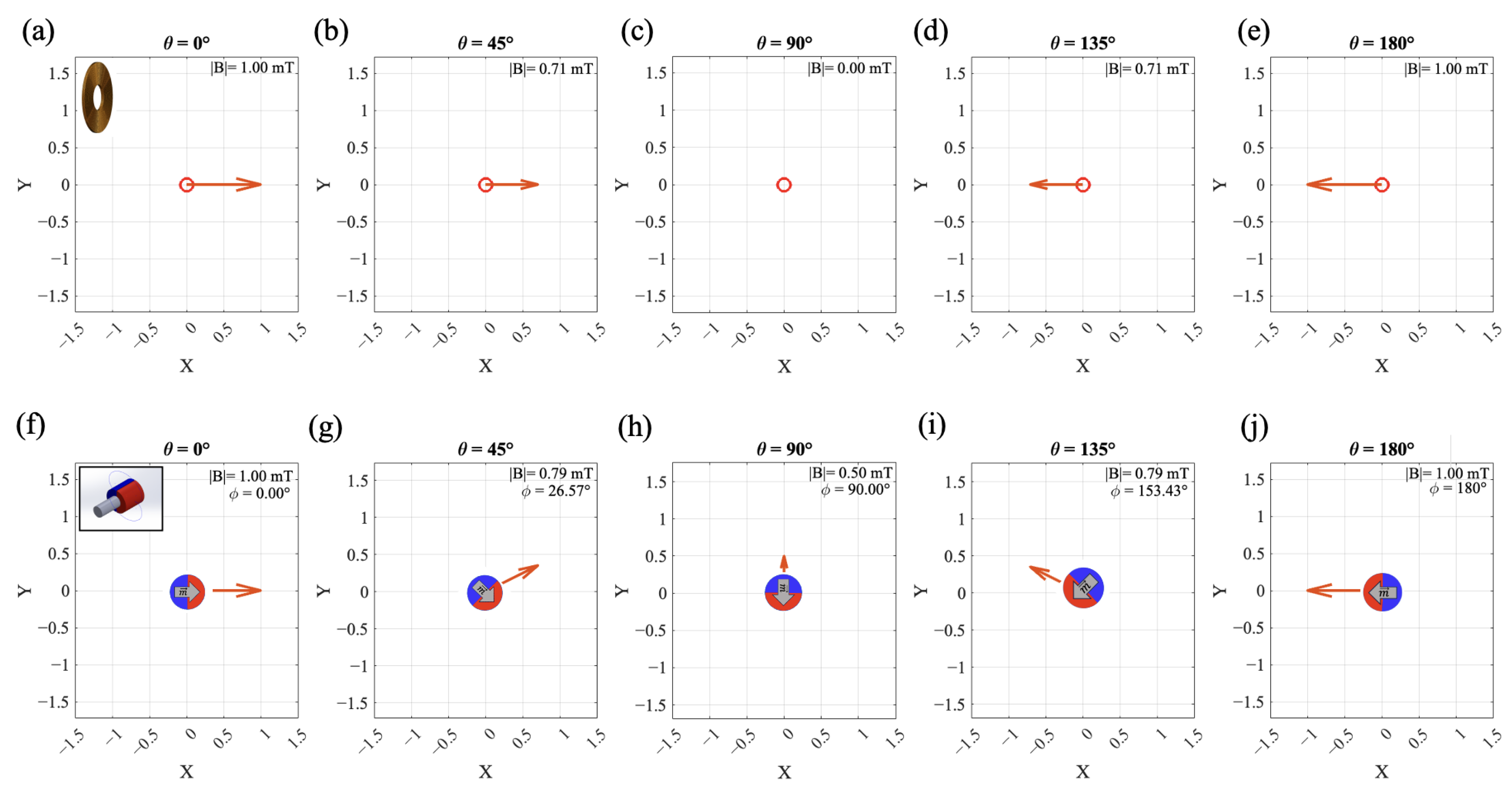
3.1.1. Uniaxial Field Case

Figure 5a shows the receiver parametrization, where a diametrically magnetized cylindrical permanent magnet in the presence of an incident uniaxial magnetic field rotates about the z-axis. At the receiver, a time-varying uniaxial magnetic B-field is produced by injecting a sinusoidal AC current at a frequency $f_e$ into the transmitter coil. The current maximum amplitude is assumed to be time-invariant for this derivation. The uniaxial sinusoidal magnetic flux density, assumed to be homogeneous over the entire receiver magnet, has an amplitude $B_0$ and an electrical angular frequency, ${\omega }_e=2\pi f_e$

$$\overrightarrow{B}\left(t\right)=B_0\cos \left({\omega }_{e}t\right)\widehat{\mathbf{x}}.$$

(1)

The direction of the magnetic field is fixed along the x-axis and taken as a reference, from which other system parameters, such as angles, are referenced. The magnetic moment $\overrightarrow{m}$ of the magnet is expressed as follows:

$$\overrightarrow{m}=M_{r}Vol[\cos \left({\theta }_m\right)\widehat{\mathbf{x}}+\sin \left({\theta }_m\right)]\widehat{\mathbf{y}}.$$

(2)

where ${\theta }_m$ is arbitrary rotation angle of the receiver magnet, $M_r$ is the remanent magnetization of the magnet and $Vol=\pi D_m^2{L}_m/4$ is the volume of the receiver magnet, expressed in terms of the diameter $D_m$ and length $L_m$. The interaction between the transmitter field and the receiver magnet results in a magnetic torque acting on the receiver magnet:

$${\overrightarrow{\tau }}_{mag}^{uni}=\overrightarrow{m}\times \overrightarrow{B}=-B_0{M}_{r}Vol\cos \left({\omega }_{e}t\right)\sin \left({\theta }_m\right)\widehat{\mathbf{z}}$$

(3)

For the uniaxial case, an imaginary rotating vector $\overrightarrow{P}$ is introduced to define a phase reference. $\overrightarrow{P}$ has an instantaneous angle of ${\theta }_t={\omega }_{e}t$ with respect to the x-axis such that the projection of $\overrightarrow{P}$ onto the x-axis gives the real uniaxial magnetic field. The superscript ’uni’ used in Equation (3) indicates the magnetic torque pertaining to the uniaxial case and differs from the biaxial case. Now, the receiver coil wound around the receiver magnet is considered. A reference angle $\alpha$ is taken between the axis of the pick-up coil and the x-axis. The rotational motion of the receiver magnet generates an alternately varying flux in the coil. The electrodynamic coupling between the pick-up coil and the receiver magnet, defined in [11], relates the induced voltage emf in the coil to the angular velocity of the magnet and, similarly, the coil current to the current induced torque and is given by the electrodynamic transduction coefficient:

$$K=K_0\sin ({\theta }_m-\alpha )={\displaystyle \frac{V_{emf}}{\dot{\theta }}}=-{\displaystyle \frac{{\tau }_{coil}}{i_{coil}}}$$

(4)

where $K_0$ is the proportionality factor. $V_{emf}$ is the induced voltage in the receiver coil, $i_{coil}$ is the current flowing in the receiver coil, and ${\tau }_{coil}$ is the magnitude of the current-induced torque. The negative sign associated with the induced torque indicates the opposing effect on rotation. In the absence of an iron core and due to lower operating frequencies, the coil is assumed to be purely resistive (${\omega }_L<<R_{coil}$). With the coil connected to a resistive load $R_L$, the voltage and currents are related by the following expression:

$$i_{coil}={\displaystyle \frac{V_{emf}}{R_{coil}+R_L}}={\displaystyle \frac{K_0{\dot{\theta }}_m}{R_{coil}+R_L}}={\displaystyle \frac{K_0}{R_{coil}+R_L}}\sin ({\theta }_m-\alpha ){\dot{\theta }}_m$$

(5)

From (4) and (5), we obtain

$${\tau }_{coil}=-K{i}_{coil}=-{\displaystyle \frac{K_0^2}{R_{coil}+R_L}}{\sin }^2({\theta }_m-\alpha ){\dot{\theta }}_m=-c_{em}{\dot{\theta }}_m$$

(6)

The final second-order equation resulting from the interaction of all the torques is given by

$$J\ddot{\theta }+[c+c_{em}]{\dot{\theta }}_m+B_0{M}_{r}Vol\sin \left({\theta }_m\right)\cos \left({\omega }_{e}t\right)=0$$

(7)

where J is the mass moment of inertia of the receiver magnet c is the viscous damping, $c_{em}$ is the electromechanical damping, defined as $c_{em}={\displaystyle \frac{K_0^2}{R_{coil}+R_L}}{\sin }^2({\theta }_m-\alpha )$, where $K_0$ is the electrodynamic transduction coefficient that relates induced voltage $V_{emf}$ to the angular velocity of the magnet, ${\dot{\theta }}_m$. $R_{coil}$ is the resistance across the receiver coil, $R_L$ is the resistive load chosen and $\alpha$, and is the reference angle of the coil in reference to the x-axis. The above Equation (7) can be solved to extract the velocity of the receiver permanent magnet and other system variables.

Open-circuit solution: In Equation (7), a constant angular velocity (i.e., zero acceleration) lacks a steady-state solution. The mechanical frequency, phase relationship between the incident field and the magnetic moment of the magnet, and torque exhibit both mean and fluctuation components. A first-order approximation of the pull-out frequency for the open circuit case is given by [11]

$${\omega }_{lim}^{uni}(R_L\to \infty )={\displaystyle \frac{B_0{M}_{r}Vol}{2c}}$$

(8)

As observed in Equation (8), the maximum operating open-circuit angular frequency (given by the condition $R_L\to \infty$) is dependent on the magnitude of the transmitter B-field, $B_0$, the magnetic material remanence of the receiver magnet $M_R$, the volume of the permanent magnet, $Vol$ and the mechanical damping coefficient c.

Matched-load solution: For the receiver connected to the load resistor, currents induced due to the rotating magnet flow through the resistor along the coil and generate an opposing electromagnetic torque on the magnet. At lower resistive loads, the pull-out frequency is minimal, nearly resembling a short-circuit condition. As the resistive load is increased, the pull-out frequency increases, and the current flowing in the resistor is minimal, resulting in the least electromechanical damping, identical to the open-circuit condition. At the first order, the mean value of the electromechanical damping term can be considered ${\overline{c}}_{em}={\displaystyle \frac{K_0^2}{2(R_{coil}+R_L)}}$. As a consequence, the pull-out frequency of the electrically loaded system is a combination of the damping from the roller bearings and the mean electromechanical damping [11]:

$${\omega }_{lim}^{uni}\left(R_L\right)={\displaystyle \frac{B_0{M}_{r}Vol}{2(c+\frac{K_0^2}{2(R_{coil}+R_L)})}}$$

(9)

which, compared to Equation (8), is additionally dependent on the electrodynamic coupling between the permanent magnet and the windings, the winding resistance and the resistive load.

3.1.2. Biaxial Field Case

A permanent magnet of fixed magnetic moment with an increasing velocity is assumed for the rotating magnet transmitter. The rotating magnetic field is modeled as a biaxial field with orientation in the x/y plane. Figure 5b shows a diametrically magnetized cylindrical permanent magnet that is designed to rotate about the z-axis and is in the presence of a biaxial field from a rotating magnet transmitter. Similar to the uniaxial field problem, the magnetic field is assumed to be homogeneous over the entire receiver magnet. The incident magnetic field at the location of the receiver is represented as,

$$\overrightarrow{B}\left(t\right)=B_x\cos \left({\theta }_t\right)\widehat{\mathbf{x}}+B_y\sin \left({\theta }_t\right)\widehat{\mathbf{y}}$$

(10)

where the rotating magnetic field is expressed as a biaxial field. Assuming that the transmitter magnet behaves as a magnetic dipole, with $B_0={\displaystyle \frac{{\mu }_0{m}_{T_x}}{2\pi d^3}}$, where $m_{T_x}$ is the magnetic moment of the permanent magnet of the permanent magnet in the transmitter. The field is observed at the receiver from a sufficiently large distance ($d>>Vo{l}_{T_x}$). The above equation is rewritten in the form [2],

$$\overrightarrow{B}\left(t\right)=B_0\cos \left({\theta }_t\right)\widehat{\mathbf{x}}-{\displaystyle \frac{B_0}{2}}\sin \left({\theta }_t\right)\widehat{\mathbf{y}}$$

(11)

where $B_0$ is the amplitude of the magnetic flux density in the $\widehat{x}$ direction, $B_0/2$ is the amplitude in the $\widehat{y}$ direction [2], and ${\theta }_t$ is the angular position of the transmitter magnet about the $\widehat{z}$ axis. A negative sign is assigned to the y component due to the opposite direction of the field lines at the point of the receiver. The expression for the magnetic moment $\overrightarrow{m}$ is unchanged and is the same as Equation (2). For the biaxial field scenario, the angle $\phi$ defined as

$$\phi ={\theta }_p-{\theta }_m=-{\theta }_t-{\theta }_m$$

(12)

is the physical lag between the imaginary vector $\overrightarrow{P}$ linked to the transmitter magnetic moment angular position ${\theta }_t$, and the angle of the rotating magnet represented by the reference position of the magnetic moment ${\theta }_m$. The interaction of the transmitter magnetic field and the magnetic moment creates a magnetic torque acting on the receiver magnet:

$${\overrightarrow{\tau }}_{mag}^{bi}=-B_0{M}_{r}Vol[\cos \left({\theta }_t\right)\sin \left({\theta }_m\right)+{\displaystyle \frac{1}{2}}\sin \left({\theta }_t\right)\cos \left({\theta }_m\right)]\widehat{\mathbf{z}}$$

(13)

As seen in the above equation for the magnetic torque, ${\overrightarrow{\tau }}_{mag}^{bi}$ is a time-varying entity and has both positive and negative values. It is noted that compared to Equation (3), an additional component surfaces due to the biaxial field when compared to the uniaxial case. The expressions for the electrodynamic transduction coefficient K, current flowing in the receiver coil, $i_{coil}$ and the magnitude of the current induced torque ${\tau }_{coil}$, given in Equations (4)–(6), are unchanged for the biaxial field case. The equation of motion resulting from the biaxial field, the induced torques and the angular moment is given by

$$J\ddot{\theta }+[c+{\displaystyle \frac{K_0^2}{(R_{coil}+R_L)}}{\sin }^2({\theta }_m-\alpha )]{\dot{\theta }}_m+B_0{M}_{r}Vol[\cos \left({\theta }_t\right)\sin \left({\theta }_m\right)+{\displaystyle \frac{1}{2}}\sin \left({\theta }_t\right)\cos \left({\theta }_m\right)]=0$$

(14)

The above equation represents the dynamic equation of the receiver when excited by the biaxial field. Equation (14) can be solved to extract parameters like the angular rate of rotation of the receiver magnet ${\dot{\theta }}_m={\omega }_m=2\pi f$ and other system parameters. Equation (14) does not have a steady-state solution where the angular rate of rotation ${\dot{\theta }}_m$ is constant, indicating zero acceleration. However, a constant phase lag is a steady-state solution in the case of a constant-amplitude rotating field. In the simulation using MATLAB, it will be proved that the angular frequency of the receiver magnet, ${\omega }_m\left(t\right)={\dot{\theta }}_m\left(t\right)$, the phase $\phi \left(t\right)$ and the torque ${\tau }_{coil}\left(t\right)$, all have a mean and a fluctuation component in the form $x\left(t\right)=x_0+∆x+\cos (2{\theta }_t+\varphi )$, where the fluctuation component is at twice the excitation frequency.

3.2. Analytical Solution

Open-circuit solution: First, the unloaded case is derived, i.e., open circuit. During the steady-state synchronous motion of the magnet (below the pull-out frequency), the angular frequency ${\omega }_m$ has a mean value equal to the excitation frequency ${\omega }_t$ and a fluctuating component $∆{\omega }_t$.

$${\omega }_m={\omega }_t-∆\omega \cos (2{\theta }_t+{\varphi }_{\phi })$$

(15)

The phase lag between the transmitter and receiver magnets can be similarly expressed using a mean and fluctuation term,

$$\phi ={\phi }_0-∆\phi \cos (2{\theta }_t+{\varphi }_{\phi })$$

(16)

The fluctuations in both 15 and 16 represent the periodic acceleration and deceleration of the magnet. The equation of motion 14 is rewritten in terms of $\phi$ and then further developed in terms of ${\phi }_0$, $∆\phi$ and ${\varphi }_{\phi }$ using Equation (16). It can be assumed that the fluctuations $∆\phi$ are much smaller than 1, especially at high frequency (i.e., $∆\phi <<1$). The rewritten equation is then arranged in terms of 1, $\cos \left(2{\theta }_t\right)$, $\sin \left(2{\theta }_t\right)$ and each corresponding coordinate term is equated to zero to verify the equation for any given instant. From this, the mean phase lag and the pull-out frequency can be determined. For synchronous operation, the mean-phase lag for the biaxial field case is given by

$${\phi }_0=arcsin\left({\displaystyle \frac{{\omega }_t}{{\omega }_{lim}}}\right)$$

(17)

where ${\phi }_0$ ranges from 0 at low frequencies to $\pi /2$ at the pull-out frequency, which at the open circuit condition is then found to be

$${\omega }_{lim}^{bi}(R_L\to \infty )={\displaystyle \frac{3}{2}}{\displaystyle \frac{B_0{M}_{r}Vol}{2c}}$$

(18)

By comparing Equations (5) and (18), it can be noted that the open circuit pull-out frequency (given by the condition $R_L\to \infty$), for the biaxial field case, is 50% higher than the uniaxial field case. This increase in pull-out frequency results in a higher operating frequency, leading to higher induced voltages.

Matched-load condition: Similarly to the uniaxial case, the pull-out frequency for the biaxial field case when connected across a matched load is given by

$${\omega }_{lim}^{bi}\left(R_L\right)={\displaystyle \frac{3}{2}}{\displaystyle \frac{B_0{M}_{r}Vol}{2(c+\frac{K_0^2}{2(R_{coil}+R_L)})}}$$

(19)

which, compared to Equation (18), is additionally dependent on the electrodynamic coupling between the permanent magnet and the windings, the winding resistance, and the resistive load $R_L$. By comparing Equations (9) and (19), we observed that the loaded pull-out frequency ${\omega }_{lim}^{bi}\left(R_L\right)$ is also 50% larger than in the uniaxial case ${\omega }_{lim}^{uni}\left(R_L\right)$.

Theoretical maximum power: To determine the maximum time-averaged power delivered across the load, the voltage across the load is observed. The load voltage is given by the expression [11]

$$V_L\left(t\right)=i_{coil}{R}_L={\displaystyle \frac{R_L}{R_{coil}+R_L}}{K}_0\sin ({\theta }_m-\alpha ){\omega }_{lim}^{bi}$$

(20)

And the instantaneous power delivered to the load resistor is given by the expression [11]

$$P_L\left(t\right)=i_{coil}^2{R}_L={\displaystyle \frac{R_L}{{(R_{coil}+R_L)}^2}}{K}_0^2{\sin }^2({\theta }_m-\alpha ){\left({\omega }_{lim}^{bi}\right)}^2$$

(21)

The time-averaged power can then be calculated from (21). The mean square of the electrodynamic coupling coefficient, averaged over one full rotation, is equal to $\overline{K^2}=\overline{K_0^2{\sin }^2({\theta }_m-\alpha )}=K_0^2/2$. The time-averaged power delivered to the load is given by,

$$P_L=\overline{P_L\left(t\right)}={\displaystyle \frac{K_0^2{R}_L}{2{(R_{coil}+R_L)}^2}}{\left({\omega }_{lim}^{bi}\right)}^2$$

(22)

At the pull-out frequency ${\omega }_m\approx {\omega }_{lim}^{bi}$ at which maximum power transfer occurs. The maximum power transfer that occurs at pull-out is given by,

$$P_L={\displaystyle \frac{K_0^2{R}_L}{2{(R_{coil}+R_L)}^2}}{({\displaystyle \frac{3}{2}})}^2{\displaystyle \frac{{\left(B_0{M}_{r}Vol\right)}^2}{4{(c+\frac{K_0^2}{2(R_{coil}+R_L)})}^2}}$$

(23)

Analytically, the biaxial field case ideally estimates a 2.25 times higher time-averaged power output compared to the uniaxial field.

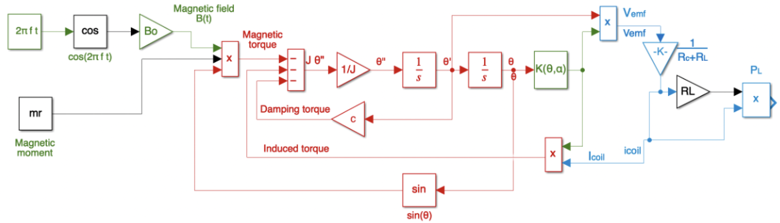
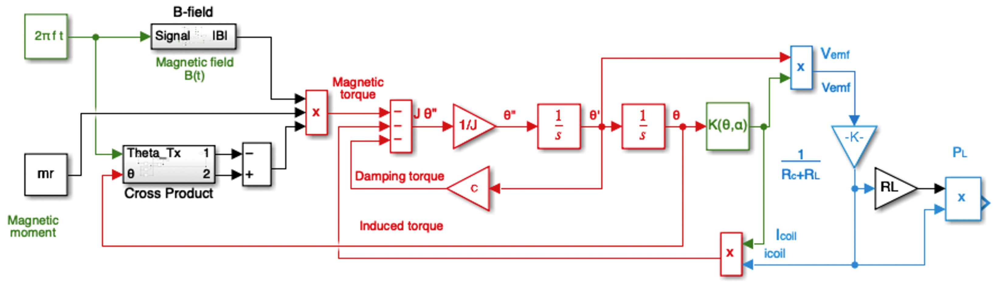
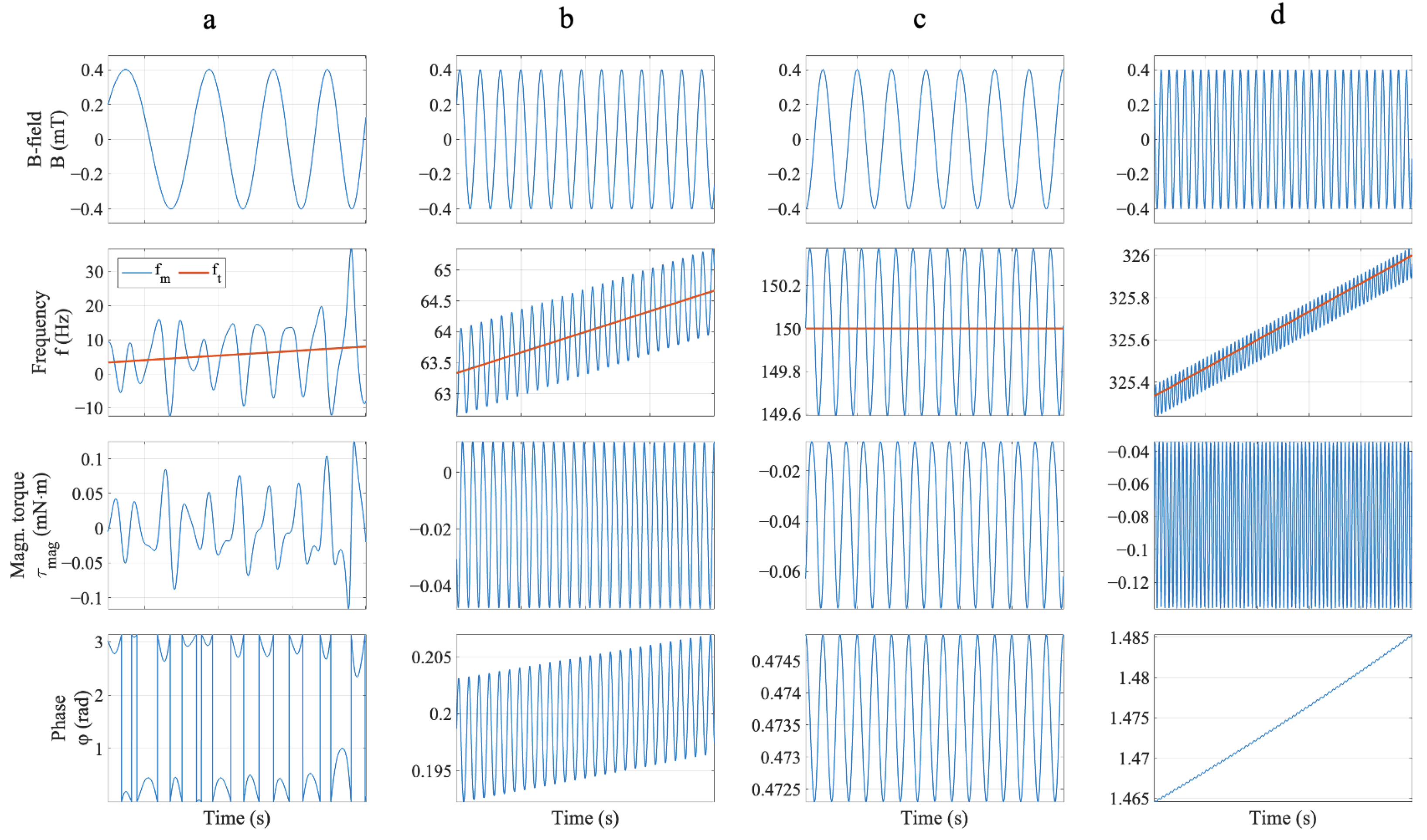
3.3. Simulink Modeling

The equations of motion, Equation (7) for uniaxial and Equation (14) for biaxial, are modeled in MATLAB, and illustrated by the Simulink block diagram in Figure 6 and Figure 7, respectively. Input parameters like the amplitude of the incident B-field at the point of the receiver, $B_0$, and the drive frequencies ($f_e$ for uniaxial and $f_t$ for biaxial case) are swept with time. All other variables, such as the phase angle, angular velocity and the magnetic torque, are extracted from the simulations. The Simulink modeling is initially simulated for the unloaded receiver to study the dynamics for the open-circuit case. The model is then extended to accommodate the electromechanical damping and its impact on the pull-out frequencies and output power. The Simulink modeling pertaining to the uniaxial case has been described and demonstrated previously [11].

In this paper, the biaxial field case is explored. Figure 8 indicates different parameter outputs from the Simulink simulation for the biaxial field case-B-field, frequency of the spinning receiver magnet, and magnetic torque and phase. A 0.401 $m{T}_{pk}$ constant-amplitude sinusoidal excitation field is used to ramp from 1 Hz to 150 Hz at 6 Hz/s for 40 s to explore the steady-state behavior, followed by a second 6 Hz/s ramp up to 400 Hz to explore the pull-out. Figure 9 shows zoomed-in versions of time intervals represented by labels a–d in Figure 8. Both figures illustrate the incident magnetic field, the transmitter and receiver mechanical frequencies $f_t$ and $f_m$, the magnetic torque and the phase lag between the rotating magnetic field and the magnet angle of the receiver.

At lower frequencies (around 20 Hz), the receiver permanent magnet displays a chaotic behavior that is similar to experimental observation. The magnetic angle varies between positive and negative values, indicating that the receiver magnet rotates in both clockwise and counterclockwise directions.

As the magnet locks with the field and starts rotating, the magnetic torque attains a periodic, synchronous behavior. The frequency of the magnetic torque oscillation is double that of the excitation frequency, as seen in Figure 9b. The angular velocity of the receiver magnet and the phase lag exhibit minor oscillations around a mean value. The average value of the angular velocity of the receiver magnet matches the angular velocity of the transmitter magnet. The angular oscillations of the receiver permanent magnet are consistent with the magnet’s acceleration or deceleration during the 360-degree rotation due to the magnetic torque oscillation between positive and negative values.

Figure 8 illustrates five distinct motion regimes experienced by the receiver magnet as the frequency is swept: (1) random oscillation, (2) ramp-up regime 1, (3) steady state rotation, (4) ramp-up regime 2, and (5) pull out regime. In regime 3 the excitation frequency is constant, indicating a steady-state rotation of the transmitter magnet. The mean angular velocity of the receiver is 150 Hz, plus an alternating component at the second harmonic, $2f_m$, with a peak magnitude of 0.4 Hz as seen in Figure 9c. This implies that the magnet is actually spinning at 150 ± 0.4 Hz. In the second ramp-up region, illustrated by regime 4 in Figure 8 and corresponding Figure 9d, the rotor approaches the pull-out frequency. The transient behavior and the small perturbations cause the pull-out phenomenon when the mean phase-lag reaches $\pi /2$. The pull-out behavior is explored using the second ramp-up region. The frequency pane of regime 5 in Figure 8 shows that beyond the pull-out frequency, the receiver magnet loses its synchronization with the transmitter magnet and the angular frequency of the receiver magnet rapidly decays to near zero. At these frequencies, the receiver magnet displays minor random oscillations. Analytically, the steady-state solution estimates that the pull-out phenomenon takes place when the mean phase-lag reaches $\pi /2$. Realistically, similar to the uniaxial field, the pull-out frequency can occur before a mean phase-lag of $\pi /2$ due to the effects of small perturbations and the transient behavior. The phase pane in Figure 8 illustrates the increase in phase-lag from zero at lower frequencies to close to $\pi /2$ at pull-out frequency. At the same time, the mean value of torque for the biaxial case increases from 0 at lower frequencies to $(3/2)B_0{M}_{r}Vol$ at pull-out. Beyond pull-out, higher frequencies cause small-scale vibrations in the magnet, but no continuous rotation is observed.

For a given amplitude of the transmitter field, $B_0$, the uniaxial and the biaxial field cases are simulated and compared in Figure 10. At a field of 0.401 mT, the receiver driven by the uniaxial field spins up to 234 Hz as seen in Figure 10a while in Figure 10b, the receiver driven by the biaxial field spins to 332 Hz, indicating 42% higher frequency compared to the receiver driven by the uniaxial field. This increase in pull-out frequency leads to increased induced voltages, resulting in higher power output. It is noteworthy that while the analytical reasoning predicts the pull-out frequency to be 50% higher for the biaxial field case over the uniaxial field case, without considering any transients, simulation results indicate the pull-out frequency for the biaxial field case to be an average of 45% higher than the simulation results for the uniaxial field. This is due to the small perturbations and transient behavior which cause pull-out before the mean phase-lag of $\pi /2$ is reached, which is well captured by the simulation.

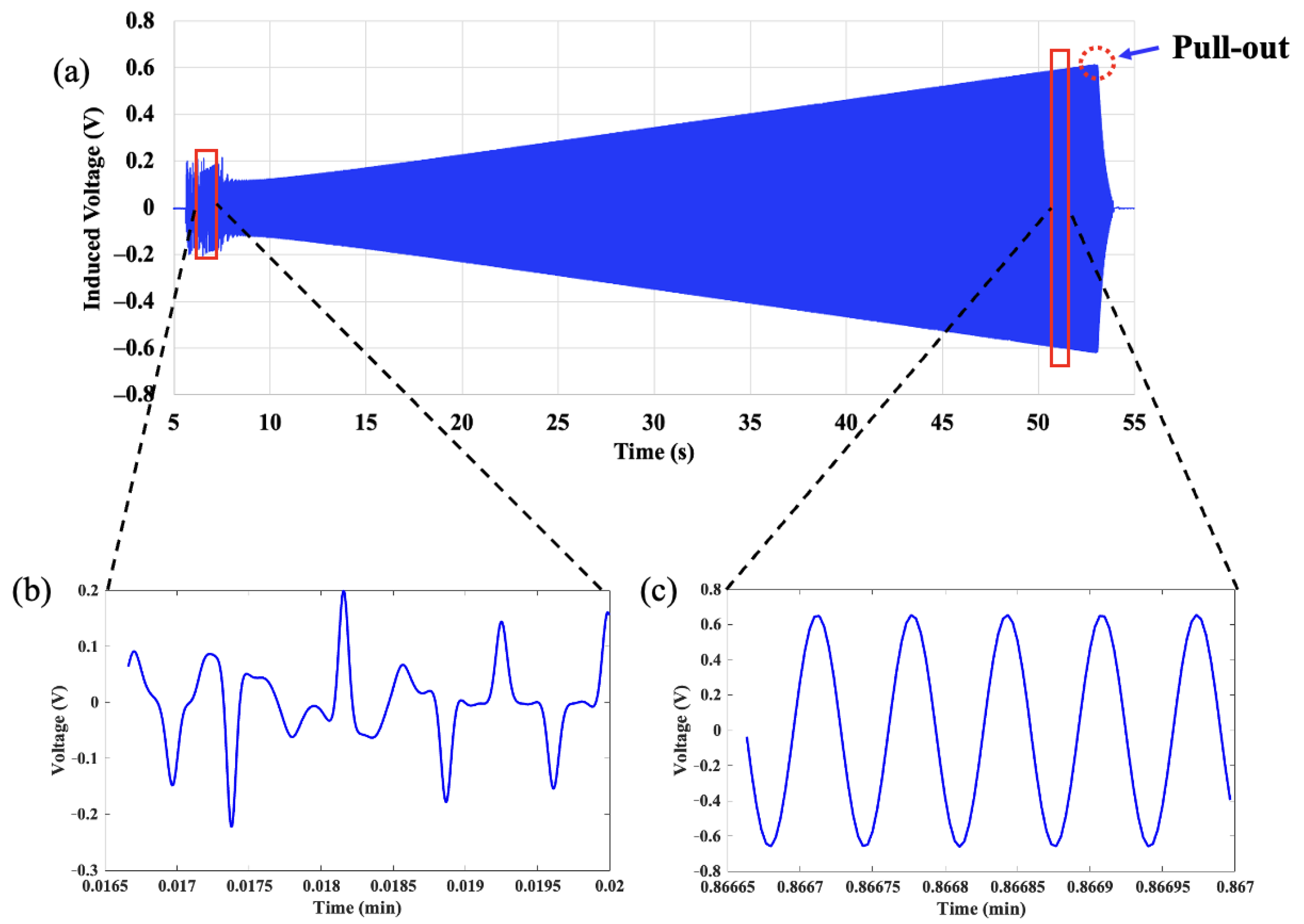
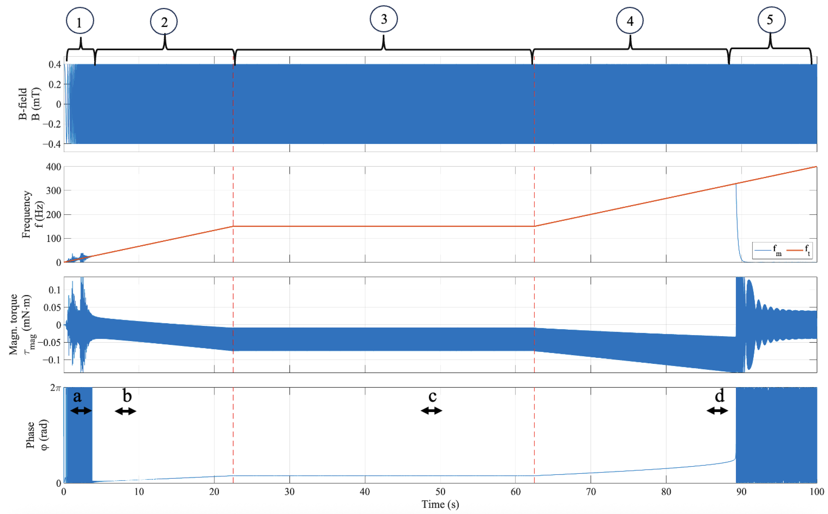
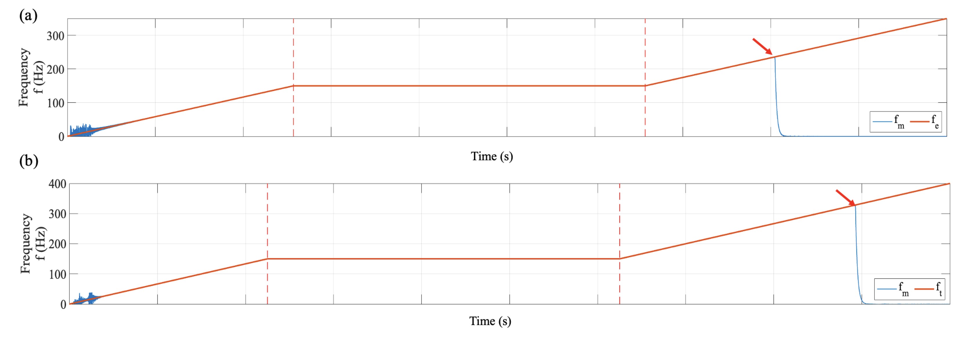
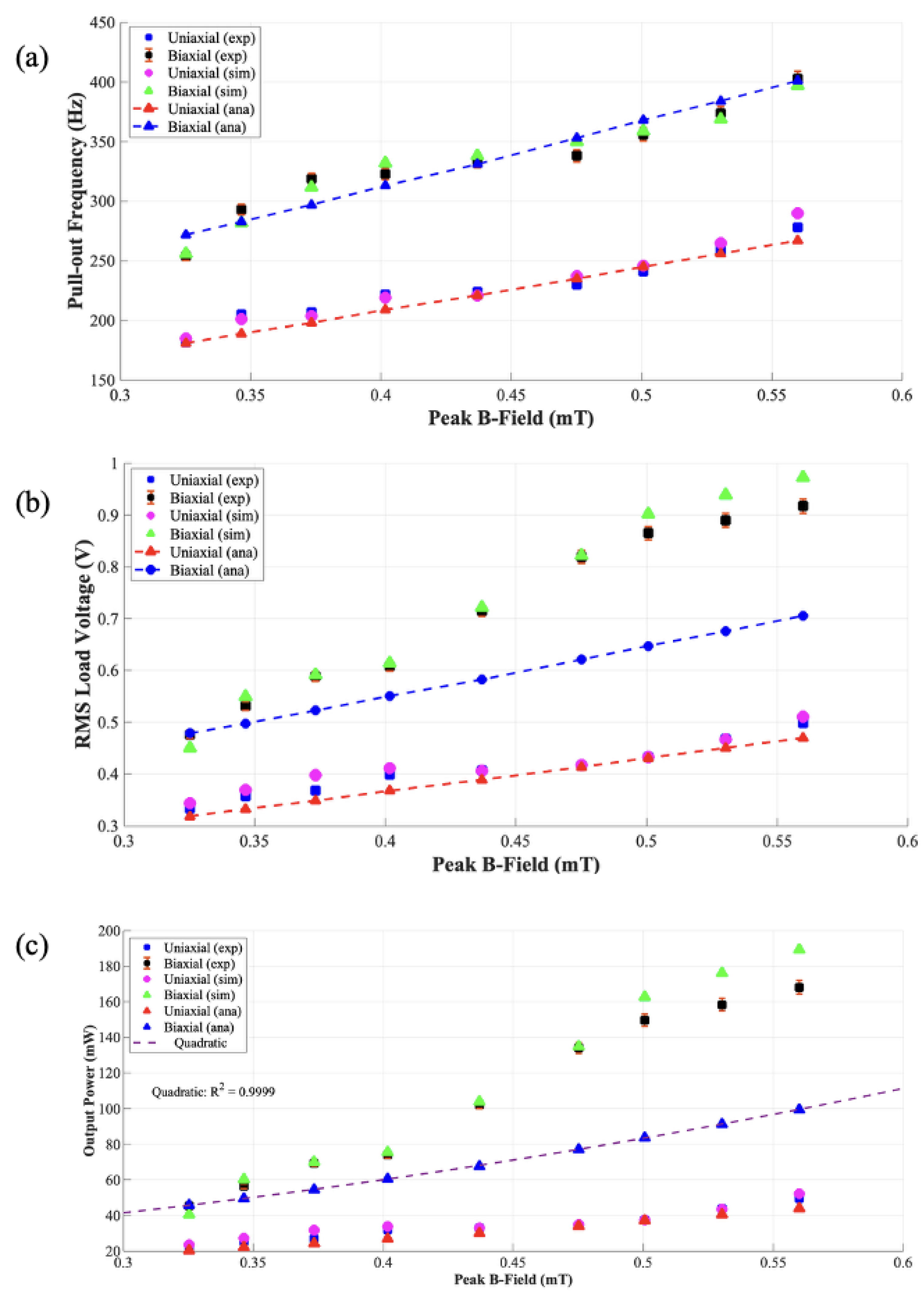
4. Experimental Results and Discussion

The receiver was placed at varying distances from the rotating magnet transmitter, ranging from 13 cm to 11 cm, to simulate B-field amplitudes between 325 µT and 560 µT and evaluate the performance characteristics. Beyond 13 cm or at fields below 325 µT, the field from the rotating magnet transmitter was not strong enough to spin the receiver magnet, while below 11 cm or at fields above 560 µT, the maximum angular velocity of the rotating magnet transmitter was limited by the maximum allowable speed of the Portescap BLDC motor. In the case of the coil transmitter, the distance between the coil and the receiver was fixed at 12 cm, and the current injected into the coil was varied to imitate similar fields.

Next, the performance characteristics of the receiver are studied. With a 5 Ω load connected across the terminals 1 and 3 of the receiver in a 144° configuration, the output power dissipated across the load was measured. At an incident field of 501 µT, the receiver generated 149 mW at 356 Hz with the rotating magnet transmitter, when it generated 38 mW at 241 Hz with the coil transmitter. For both the uniaxial and the biaxial field cases using the coil transmitter and the rotating magnet transmitter, respectively, the pull-out frequencies for different amplitudes of B-field determined through experiments, simulation and analytical approaches are plotted in Figure 11a. The analytical, simulation and experimental results for the pull-out frequencies are closely matched. While the analytical approach for the biaxial field case indicates a constant 50% increase over the uniaxial field case, the simulations and experiments illustrate an average of 45% and 46% increase, respectively.

Figure 11b shows the experimental, simulated and analytical load voltages for the uniaxial and biaxial cases. The increase in pull-out frequencies for the biaxial field over the uniaxial field contributes to the increase in the corresponding load voltages. It is interesting to note that while experimentally $K_0$ was found to increase from 280 µV-s/rad to 415 µV-s/rad across different B-fields, for the analytical case, the minimum value of 280 µV-s/rad was chosen. The power outputs at different B-fields for the experimental case, along with the simulated and the analytical results, are illustrated in Figure 11c. At a field of 501 µT, the receiver driven by the rotating magnet receiver and loaded with a resistor across nodes 1–3, in a 144° fashion produces 149 mW, resulting in a superior normalized power density [$NPD=P_{out}/(Vol.\times B_{pk}^2)$] of 543 mW/cm³/mT², which is the highest reported value. Although the output power varies quadratically with the B-field as seen in Equation (23), the quadratic trend in Figure 11c is not readily apparent due to the narrow range of B-field values at which the receiver was tested. Each experimental data point corresponds to the mean of three measurements, with the error bars indicating a 95% confidence interval. Analytically, the pull-out frequency for the biaxial field case is determined to be 50% higher than the uniaxial field case. Since the induced voltage is linearly related to the pull-out frequencies, it also illustrates a 50% higher increase for the biaxial field case over the uniaxial field case.

However, at strong fields, the experimentally measured induced voltages deviate from the linear trend, exhibiting an S-type behavior, with an average increase of 72% over the uniaxial field case. This may be attributed to a couple of factors. Firstly, Equation (11) assumes that the magnetic field originating transmitter magnet is observed from a far-off distance and the magnet is treated as a dipole. But with strong fields, the receiver is likely closer to the magnet, which could cause the dipole approximation to break down. This proximity effect may further explain the observed deviations in the induced voltage and power output trends. This can be further explored and simulated using software packages like COMSOL. Secondly, the biaxial field assumption from Equation (11) assumes a non-constant rotating magnetic field, resulting in a 50% increase and lies between a uniaxial field and a constant amplitude rotating magnetic field, and the pull-out frequencies can approach twice that of the uniaxial magnetic field, predicting 4× times higher power.

The 46% increase in pull-out frequencies, 72% higher induced voltages and three times higher power output for the biaxial field case demonstrated by the rotating magnet transmitter, is attributed to the additional component of field along the y direction.

5. Conclusions

In this work, an EWPT receiver with a rotating permanent magnet is observed under the influence of a uniaxial B-field and a rotating B-field modeled as a non-constant amplitude biaxial field. The equations of motion are derived in both cases and are modeled in MATLAB and Simulink to obtain the output parameters: angular velocity of the receiver, magnetic torque and the phase lag between the transmitter and receiver. The analytical, simulation and experimental results are studied for the rotating magnet transmitter that generates a biaxial field.

Further, the pull-out frequencies, load voltages and the output power for both cases are compared. The EWPT receiver driven by a rotating magnet transmitter that simulates a rotating (biaxial) magnetic field outperforms the uniaxial field demonstrated by the coil-based transmitter. At identical fields of 501 µT, the receiver driven by the coil transmitter transfers 38 mW while the receiver driven by the rotating magnet transmitter delivers 149 mW, illustrating a 3.9 times increase over the coil transmitter. This translates for the rotating magnet transmitter to a power density [$PD=P_{out}/Vol.$] of 136 mW/cm³ and an NPD of 543 mW/cm³/mT², which is the highest reported value. The experimental power transfer efficiency was observed to be 0.96% for the rotating magnet transmitter and 0.16% for the coil transmitter, indicating a six times improvement from the coil transmitter. The rotating magnet transmitter offers higher pull-out frequencies, induced voltages, and output power, leading to better normalized power densities and efficiencies. The better performance with the rotating magnet transmitter is simply due to higher pull-out frequencies, which are attributed to the rotating magnetic field. However, there are practical limits to rotating magnet transmitters, namely the maximum operational speeds/frequencies. Whereas it is relatively trivial to create a 1 kHz sinusoidal field variation using electric currents in a coil, achieving that frequency by mechanically rotating a magnet requires a spin speed of 60,000 rpm. Such speeds push the limits of typical low-cost electrical motors and rotational bearings.

Overall, EWPT represents a promising alternative to traditional inductive wireless power transfer methods. Its low frequency of operation makes it less susceptible to interference, moisture, conductive materials, salinity, etc., thus making it a compelling option for applications such as IoT infrastructure where reliability and efficiency are paramount.

References

1. Niu, S.; Xu, H.; Sun, Z.; Shao, Z.; Jian, L. The state-of-the-arts of wireless electric vehicle charging via magnetic resonance: Principles, standards and core technologies. Renew. Sustain. Energy Rev. 2019, 114, 109302. [Google Scholar] [CrossRef]
2. Li, W. High Efficiency Wireless Power Transmission at Low Frequency Using Permanent Magnet Coupling. Ph.D. Thesis, University of British Columbia, Vancouver, BC, Canada, 2009. [Google Scholar] [CrossRef]
3. Du, S.; Chan, E.K.; Wen, B.; Hong, J.; Widmer, H.; Wheatley, C.E. Wireless Power Transfer Using Oscillating Magnets. IEEE Trans. Ind. Electron. 2018, 65, 6259–6269. [Google Scholar] [CrossRef]
4. Singer, A.; Dutta, S.; Lewis, E.; Chen, Z.; Chen, J.C.; Verma, N.; Avants, B.; Feldman, A.K.; O’Malley, J.; Beierlein, M.; et al. Magnetoelectric Materials for Miniature, Wireless Neural Stimulation at Therapeutic Frequencies. Neuron 2020, 107, 631–643.e5. [Google Scholar] [CrossRef] [PubMed]
5. Barrett, C.; Fu, H.; Theodossiades, S. Electrodynamic Wireless Power and Data Transfer for Implanted Medical Devices. In Proceedings of the 2023 IEEE SENSORS, Vienna, Austria, 29 October–1 November 2023; pp. 1–4. [Google Scholar] [CrossRef]
6. Garraud, N.; Alabi, D.; Chyczewski, S.; Varela, J.D.; Arnold, D.P.; Garraud, A. Extending the range of wireless power transmission for bio-implants and wearables. J. Phys. Conf. Ser. 2018, 1052, 012023. [Google Scholar] [CrossRef]
7. Garraud, N.; Alessandri, B.; Gasnier, P.; Arnold, D.; Boisseau, S. Optimization of a Magnetodynamic Receiver for Versatile Low-Frequency Wireless Power Transfer. In Proceedings of the 2019 19th International Conference on Micro and Nanotechnology for Power Generation and Energy Conversion Applications (PowerMEMS), Krakow, Poland, 2–6 December 2019; pp. 1–6. [Google Scholar] [CrossRef]
8. Jiang, H.; Zhang, J.; Lan, D.; Chao, K.K.; Liou, S.; Shahnasser, H.; Fechter, R.; Hirose, S.; Harrison, M.; Roy, S. A Low-Frequency Versatile Wireless Power Transfer Technology for Biomedical Implants. IEEE Trans. Biomed. Circuits Syst. 2013, 7, 526–535. [Google Scholar] [CrossRef] [PubMed]
9. Wu, Y.; Yuan, H.; Zhang, R.; Yang, A.; Wang, X.; Rong, M. Low-Frequency Wireless Power Transfer Via Rotating Permanent Magnets. IEEE Trans. Ind. Electron. 2022, 69, 10656–10665. [Google Scholar] [CrossRef]
10. Crasto, V.S.; Stormant, M.G.; Arnold, D.P. Electrodynamic Wireless Power Transfer to High-Performance Rotating Magnet Receivers. In Proceedings of the 2023 IEEE 22nd International Conference on Micro and Nanotechnology for Power Generation and Energy Conversion Applications (PowerMEMS), Abu Dhabi, United Arab Emirates, 11–14 December 2023; pp. 33–36. [Google Scholar] [CrossRef]
11. Garraud, N.; Garraud, A.; Munzer, D.; Althar, M.; Arnold, D.P. Modeling and experimental analysis of rotating magnet receivers for electrodynamic wireless power transmission. J. Phys. D Appl. Phys. 2019, 52, 185501. [Google Scholar] [CrossRef]
Figure 1. Overview of an electrodynamic wireless power transfer system. Both (a) a current-carrying coil transmitter and (b) a rotating magnet transmitter driven by a motor can be used to generate a time-varying field to drive the (c) EWPT receiver to transfer power. The construction of the EWPT receiver is shown in (dg).
Energies 18 02506 g001
Figure 2. The figures above show the B-fields generated by the transmitter at the receiver’s location, normalized to a unit B-field magnitude ( B 0 = 1 ). The coil transmitter produced a uniaxial field, as described by Equation (1), shown in (ae), where the field magnitude varies in a bipolar manner. In contrast, the rotating magnet transmitter generates a rotating magnetic field with a non-constant amplitude, as represented by Equation (10) and illustrated in figures (fj).
Energies 18 02506 g002
Figure 3. Experimental setup consisting of an EWPT receiver separately driven by (a) a coil transmitter and (b) a rotating magnet transmitter. (c) The rotating magnet transmitter consists of a speed controller, BLDC motor and a permanent magnet housed in a precision-machined aluminum carriage.
Energies 18 02506 g003
Figure 4. (a) Experimentally measured output voltage across a load connected to the receiver coil as a function of time. (b) Random magnet oscillations at low frequencies and (c) ramp-up region at higher frequencies, just before the pull-out frequency when the magnet stops spinning, are observed.
Energies 18 02506 g004
Figure 5. Schematic of the theoretical analysis of the rotating magnet receiver excited by (a) uniaxial field and (b) biaxial field.
Energies 18 02506 g005
Figure 6. Simulink block diagram for the uniaxial field case.
Energies 18 02506 g006
Figure 7. Simulink block diagram for the biaxial field case.
Energies 18 02506 g007
Figure 8. The output parameters using Simulink shows the B-field at the location of the receiver, the angular frequency of the receiver magnet, the magnetic torque acting on the receiver and the phase lag between the transmitter and the receiver. During the frequency sweep, the receiver exhibits five distinct motion regimes, denoted as regions 1–5: random oscillation, ramp-up 1, steady state rotation, ramp-up 2, and eventual pull-out. Labels (a–d) indicate time intervals corresponding to parameters-B-field, frequency, magnetic torque and phase, which are examined in detail in the subsequent zoomed-in plots in Figure 9, to capture the receiver magnet’s dynamic behavior.
Energies 18 02506 g008
Figure 9. A zoomed-in version of the simulation output parameters from section (ad) from Figure 8-B-field, angular frequency, magnetic torque and the phase lag at specific instances indicated by region (a) random chaotic behavior, (b) ramp-up 1, (c) steady-state rotation, and (d) ramp-up 2.
Energies 18 02506 g009
Figure 10. For a given field, B0 = 0.401 m T p k , the pull-out frequency for the (b) biaxial field at 332 Hz, was found to be 47% higher compared to the (a) uniaxial field at 234 Hz.
Energies 18 02506 g010
Figure 11. The experimental, simulated by analytical results of (a) pull-out frequencies, (b) load voltages, and (c) output powers are compared for different amplitudes fo B-field.
Energies 18 02506 g011
Disclaimer/Publisher’s Note: The statements, opinions and data contained in all publications are solely those of the individual author(s) and contributor(s) and not of MDPI and/or the editor(s). MDPI and/or the editor(s) disclaim responsibility for any injury to people or property resulting from any ideas, methods, instructions or products referred to in the content.