1. Introduction
An air handling unit (AHU) is a machine that conditions rooms and chambers using heat exchangers [
1]. They are responsible for circulating air in houses or buildings. AHUs are components of heating, ventilation, and air conditioning (HVAC) systems. They are large metallic boxes comprising a blower, filter racks, sound attenuators, and cooling and heating coils. They are installed inside and outside buildings, with the rooftop being typical for the latter where control is a challenging task [
2,
3]. Often, they are connected to the HVAC’s ductwork [
4]. The main components of an AHU system are its casing or housing, the fan, the heating and cooling coil, filters, humidifiers, and the mixing box. The primary function is heat exchange [
5] and filtering, improving the air quality. To improve their efficiency, the design of air handling units requires studies of thermal losses due to conduction and convection [
6,
7]. Efficiency is only sometimes an easy parameter to obtain [
8]. Many factors that complicate designs are thermal bridges [
9] or parameters that are difficult to measure, such as radiation heat transfer coefficients. In this case, the type of radiation can be a limiting factor, as the surfaces do not behave the same depending on the incident wavelength. Thermal bridges are essential for the overall efficiency of the units [
10]. However, their constitution is complex [
11], and they can be a determining factor in the outcome of unity. The bridging effects are remarkable compared to low-transmission panels, thanks to vacuum-insulated panels. This is marked by regulations that need to be permanently improved due to the implications of improvements to comply with environmental regulations, such as, for instance, EU regulation 1253/2014 [
12].
Recent publications have focused on AHU optimization by control, with model predictive control [
13,
14] or large language models [
15], in order to predict and optimize the energy consumption for particular HVAC applications. Computational Fluid Dynamics have been used by Lopes et al. [
16] or Azem et al. [
17] for the analysis of the flow and pressure distribution produced by a fan inside the AHU aimed to constructive enhancement of the unit. Other authors have studied the thermal efficiency of AHU equipped with heat exchangers [
18,
19]. However, to the best of the authors’ knowledge, there are no published studies on the combined analysis with CFD and the heat transfer of the thermal efficiency of the AHU with no fans or heat exchangers.
This paper presents a simplified methodology to estimate the energy efficiency of an AHU design. The primary objective is to present a semi-empirical procedure for the estimation of energy consumption and evaluate the class of the pre-designed unit according to the European Standard EN 1886:2008 [
20]. This study involves the three known means of heat exchange: conduction, convection, and radiation [
21]. Fluid dynamic phenomena that define their efficiency must also be considered. This is especially relevant in the case of filtration efficiencies. The test conditions require applying relevant techniques in measuring the temperatures decoupled from radiative interference and temperatures on surfaces, where the effects of radiation must be considered [
22]. The results obtained with this methodology are validated both with numerical computations in a 2D model and with experimental measurements on an AHU box unit.
This paper is organized as follows. In
Section 2, a semi-empirical estimation, is presented.
Section 3 describes an experimental set-up, emphasizing the mitigation of the error that could be neglected. Numerical studies are a relevant part to be compared on the semi-empirical proposal and are validated using the experimental results. The numerical results are presented in
Section 3. Finally,
Section 4 presents an extensive discussion of comparing the results.
2. Semi-Empirical Estimation
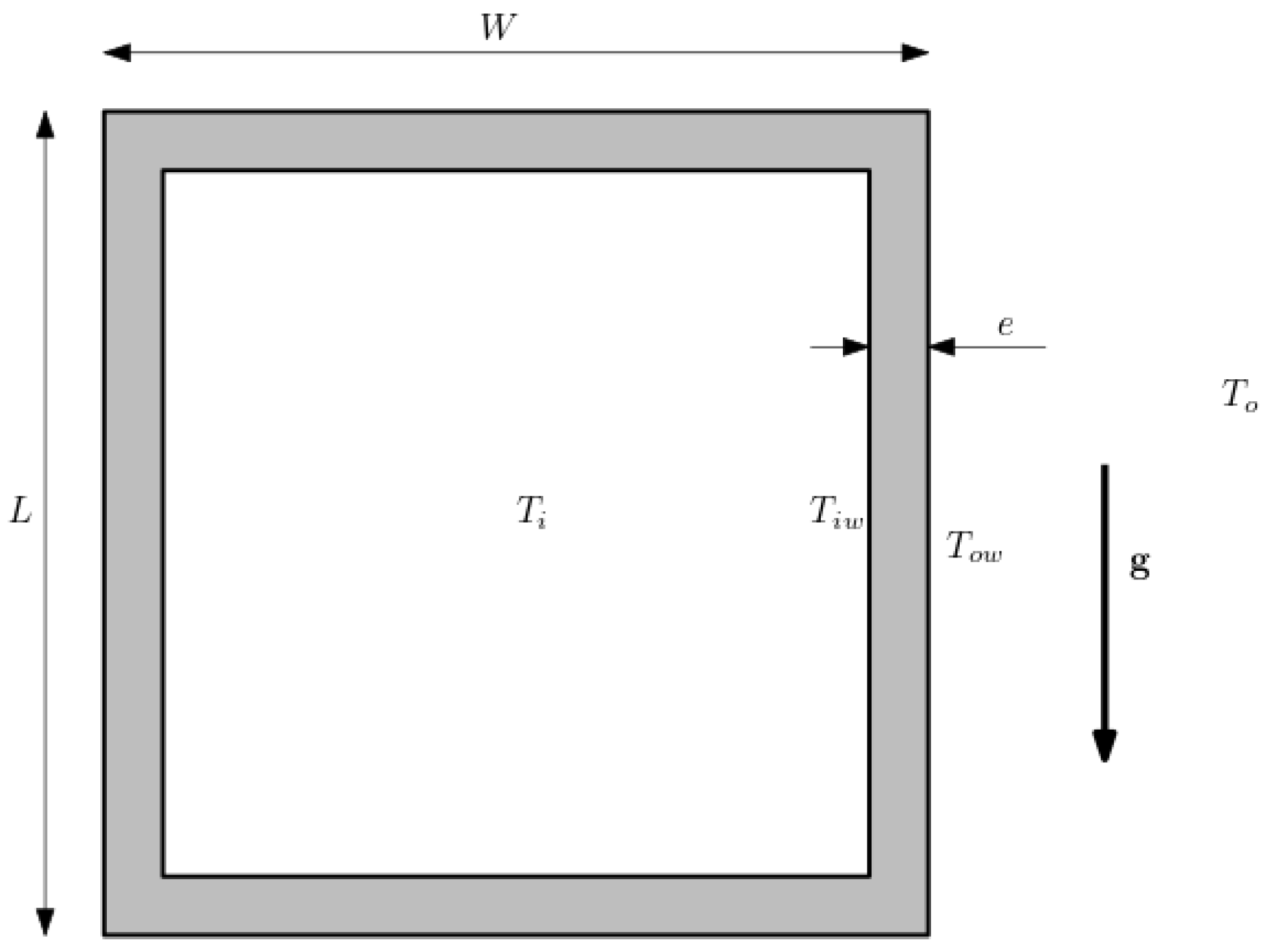
Thermal transmittance (
U) is defined as the ability of the unit to transmit heat under steady-state conditions. It is estimated as the ratio between heat transfer per area unit and the difference in temperature
where
is the total heat transfer, per unit area, and
and
are the inside and outside temperatures of the AHU, as depicted in
Figure 1. It can also be described as the sum of the reciprocals of the resistances of the elements of the unit, and is expressed in
.
The heat transmitted, per surface unit, by conduction, is given by Fourier’s law of heat conduction,
where
is the isolation thermal conductivity,
e is the wall thickness, and
and
are, respectively, the outer and inner wall temperatures (see
Figure 1) Convection heat transfer is determined with
where
h is the convection heat transfer coefficient, which does not depend exclusively on the fluid, but it is also influenced by the geometry of the surface, the nature of the fluid movement, and its average speed. Convection heat transfer coefficient is computed with the Nusselt number
where
is the thermal conductivity of the medium and
d is a characteristic length. In the following, the expressions used to estimate Nu and hence
h, have been based on the book by Çengel and Ghajar [
6], and the references therein. Convective heat transfer is estimated both inside and outside the AHU and the term
in Equation (
3) refers to the temperature difference between the wall and the far field. Outside the unit, only natural convection holds, and the Nusselt number is estimated with the expression
where
c and
n are a function of the wall orientation and the value of the outer Rayleigh number,
.
Table 1 shows the values used in the present estimation.
The Rayleigh number is computed as the product of Grashof number and Prandtl number,
where
and
where
is the viscosity of air,
is the specific heat at constant pressure,
is the thermal expansion coefficient of air,
L is the height of the unit,
g is the gravity acceleration,
is the far temperature, and
is the outside wall temperature. Hence, outer heat transfer coefficient is computed as
Note that, actually, there are three different values of depending on the orientation of the surface relative to gravity (lateral walls, top wall and bottom wall).
Inside the AHU, besides natural convection, forced convention has to be considered, due to the air circulation required by the Standard [
20] in order to keep a uniform distribution of inner temperature. The Nusselt number for the forced convection is estimated with
where
,
is the average velocity of air inside the unit and
is the hydraulic diameter. The natural convection inside the AHU is computed with the correlation found by Globe and Dropkin [
23] for a rectangular box heated from below
When both natural and forced convention are combined, the effective Nusselt number is usually estimated with [
6]
and
The heat transfer by radiation is estimated with
where
is the Stefan–Boltzmann constant and
is the effective emissivity due to the four surfaces that compose the isolation bounding walls. It is assumed that the insulator and air are transparent in the bandwidth of thermal radiation. The emissivity of the surfaces is measured with a thermographic camera.
Finally, the heat transfer in the metallic profiles of the AHU is estimated, considering only the conduction due to the metal and neglecting the effect of the air chambers.
The convective and conductive heat transfer are combined as
where
. The total heat transfer is the sum of this and the radiation term
However, this total heat transfer is function of the wall temperatures,
and
, which are, at first, unknown. This temperatures are computed with
where
where
and
are, respectively, the emissivity of the inner and outer surfaces of the AHU.
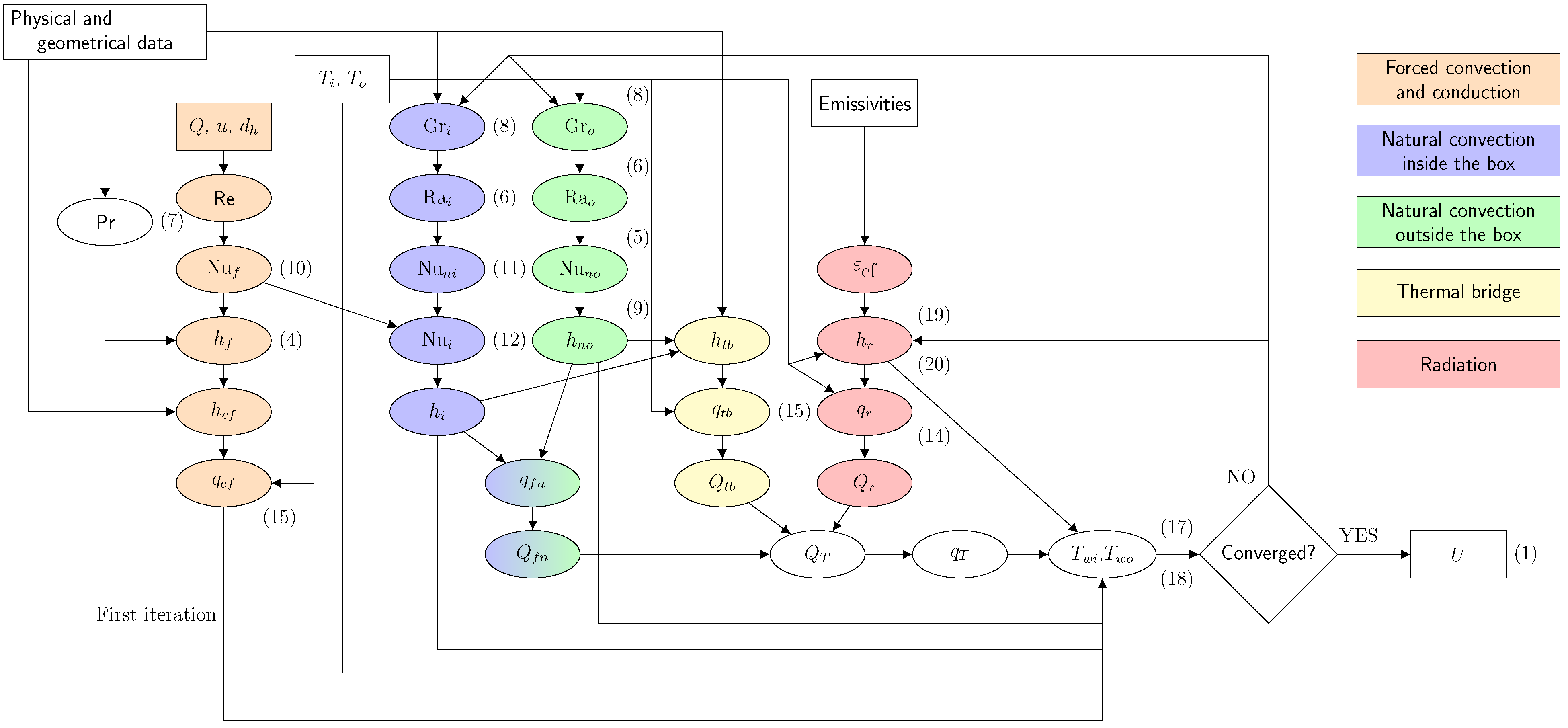
Equations (
16)–(18) are iteratively solved until a solution for
,
, and
is reached, and thermal transmittance is computed with (
1). The flowchart for this procedure is depicted in
Figure 2.
Expressions (
5), (
10), and (
11) are based on empirical statistics and, hence, are restricted to certain conditions, as infinite walls. This implies an uncertainty that has to be considered. However, the combination of natural and forced convection inside the box of the AHU, Equation (
12), can be regarded as the major source of uncertainty in the semi-empirical estimation of heat transfer by convection, according to Siebers [
24], that founded a disagreement of up to 10% with experimental data. Nevertheless, computations in the present work suggest that the radiation term in Equation (
16) is more important than convection, with approximately 80% of the total heat transfer, and it is very sensitive to the computation of surface emissivities.
The thermal bridge factor is defined in the Standard [
20] as the rate between the minimum difference of temperatures inside and in the outside wall, and the temperature difference inside and outside the AHU:
In the present estimation, since wall temperatures are considered uniform, it is computed as
3. Numerical Methodology
Numerical experiments have been performed with the toolbox OpenFOAM version 9 [
25], that uses finite volume method to solve systems of partial differential equations. The solver used has been chtMultiRegionFoam, which is used for steady or transient fluid flow and solid heat conduction. Furthermore, it conjugates heat transfer between solid and fluid regions, including buoyancy effects, turbulence, reactions, and radiation modelling. The simulations are steady, and they have been run until the convergence of heat flux is reached.
The mesh is two-dimensional for the sake of simplicity and simulation speed. It is composed of several regions that cover both fluid and solid domains. Fluid regions include the interior and exterior air spaces of the AHU, while solids consist of metallic sheets and insulation materials that form the walls of the AHU. In addition, a solid heater with constant temperature is modeled in the lower part of the inner space. Using the symmetry of the system, only half of the domain was simulated.
The mesh was generated using the
blockMesh tool included in the OpenFOAM distribution, which constructs structured hexahedral blocks. To streamline the creation of complex block configurations, the Python tool
ofblockmeshdicthelper [
26] was used.
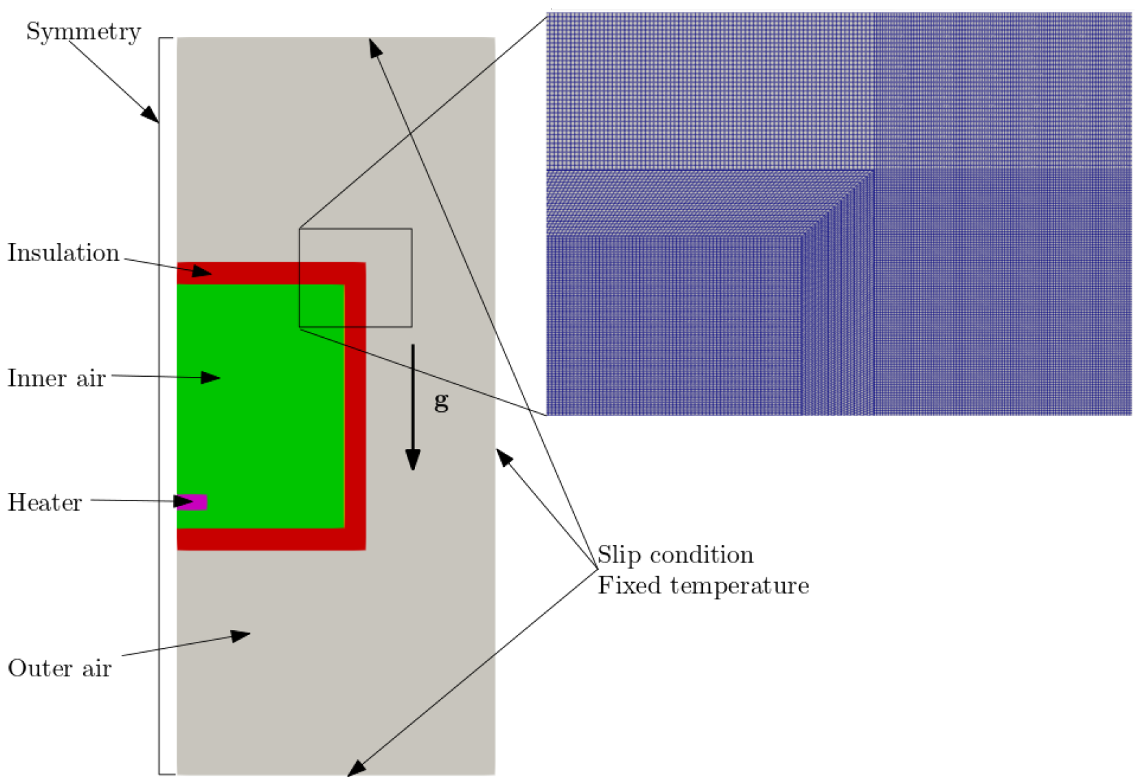
The regions considered in the simulations are the inner air, the outer air, the insulator, the metal sheets, both inner and outer, and, finally, the heater. These regions and the boundary conditions are schematically shown in
Figure 3, except metal sheets enclosing the insulation. Fifteen blocks were defined to create the structured mesh, one for the inner fluid region, nine for the three layers of metals and insulator, and finally five for the outer air region.
For the fluid regions,
chtMultiRegionFoam solves continuity equation
the momentum equation
with
, and the energy equation
where
is the density,
is the velocity,
is the pressure corrected with gravity effect,
is the stress tensor,
is the kinetic energy,
h is the enthalpy,
R is the radiation term, and
and
are, respectively, the effective viscosity and heat transfer coefficients, corrected by turbulence modeling. In the present case, standard
has been used as a turbulence model, as it has proven to be a suitable model, combining acceptable accuracy and computational resource consumption for buoyancy-driven flows [
27].
For the solid regions, only heat conduction is solved,
In the interfaces between solids and fluids, the solver imposes the same temperature
and, also, the continuity of heat transfer is ensured
For the computation of convection, air is treated as compressible with the Boussinesq approximation and the density is uniquely function of the temperature,
where
,
and
is the thermal expansion coefficient.
The radiation term
R in Equation (
25) is computed by the solver using the view factor method [
6,
21], where the radiative heat transfer is estimated by generating discrete rays between solid surfaces. For the sake of comparison, this term has been disabled on some numerical experiments.
Two series of numerical experiments have been performed. In the first series, a section of the unit has been considered and the gravity orientation has been modified in order to simulation convective heat transfer and validate semi-empirical expressions, given by the combination of Equations (
5) and (
11), for the three possible orientations of the wall, vertical, horizontal facing upwards and horizontal facing downwards. The domain used in these simulations is 2D, and composed by an external air region of
, an internal air region of
, a solid region with an insulator material, of
and 2 solid metallic sheets of
. The difference of temperatures between the inner and the outer boundaries has been set as
, specifically
end
, respectively.
Regarding the second set of numerical simulations, the whole domain with a solid heater in the centered bottom part is considered, as shown in
Figure 3. The external boundary of the domain has been defined as a wall with no-slip conditions for velocity and constant temperature. The left side of the domain has been set as a symmetry plane when radiation was disabled. However, since the view factor method does not support symmetry constraints, these boundaries have been defined as slip condition for velocity and zero gradient for other variables when radiation was enabled. The temperature of the heater solid has been established at a constant value of
. The temperature of the external boundaries was set at a value of
(see
Figure 3). A detail of the mesh is also shown in this figure.
Transmittance is numerically computed with
where the sum of heat transfers includes the heat transfer from the conduction/convection and the heat transfer from the radiation. Internal and external temperatures,
and
, are computed as the average of temperature field at a distance of 100 mm, as stated by the Standard [
20]. The thermal bridge factor is estimated using Equation (
33).
Grid Convergence Validation and Boundary Layer
The heat transfer in the inner side of the AHU has been computed for three different mesh sizes in order to assess the grid convergence, according to Celik et al. [
28]. It has been made with the second set of numerical simulations (global domain). Results are shown in
Table 2. The grid refinement ratio
r, defined as the ratio between subsequent grid sizes are 1.4 for both cases, fine to medium and medium to coarse. The grid convergence index (GCI) is computed as
where
F is a safety factor, with a typical value of 1.25, and
is the order of convergence and
are relative errors for adjacent mesh sizes. In the present case, the order of convergence is
. The extrapolated value for heat transfer, the theoretical value for infinite mesh size, is
. The values for the GCI are 0.36% for the fine mesh, 0.7% for the medium and 1.3% for the coarse one. The value of the asymptotic ratio, computed with
, is 0.997, and its closeness to 1 indicates that the meshes are in the asymptotic region and the medium mesh can be considered as valid, with an accuracy of 0.7%, that has been translated to the final results of
Section 5.
The local Reynolds number related to the boundary layer is expected to be very low, with a typical velocity of less than and a typical length scale of about 2 m, which gives . With the cell size in the walls for a medium mesh, an average value of is obtained, where is the cell center distance to the wall, is the friction velocity, is the wall friction and and are, respectively, the density and kinematic viscosity of air. According to OpenFOAM documentation, for , no wall function has to be defined in the wall and the nutLowReWallFunction boundary condition, which actually resolves the boundary layer, has been used.
4. Experimental Methodology
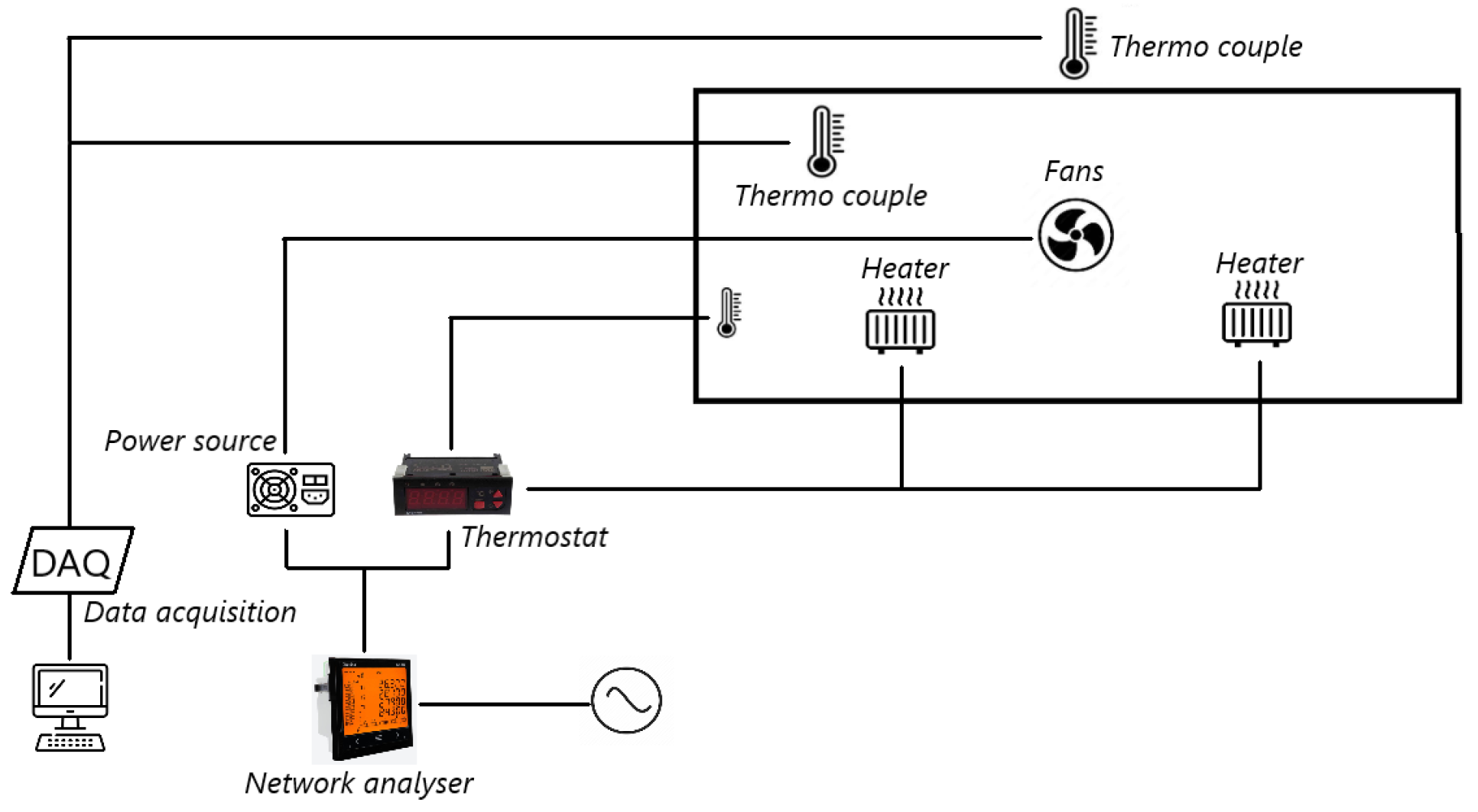
The scheme of the experimental rig is presented in
Figure 4. The generation and control of the internal temperature of the AHU, 4 axial fans, 2 heaters, and a temperature controller were installed. A Circutor CVM-C10 analyzer (Circutor, Barcelona, Spain) was used to measure the power consumed. The fans have a capacity of
each and circulate the air at about 100 AHU volumes per hour. They were installed in the middle longitudinally of the AHU to circulate the air crosswise. The heaters are electric resistance type and each have a capacity of 400 W. They are regulated by an ON/OFF temperature controller. It is equipped with an NTC temperature sensor which is located inside the unit.
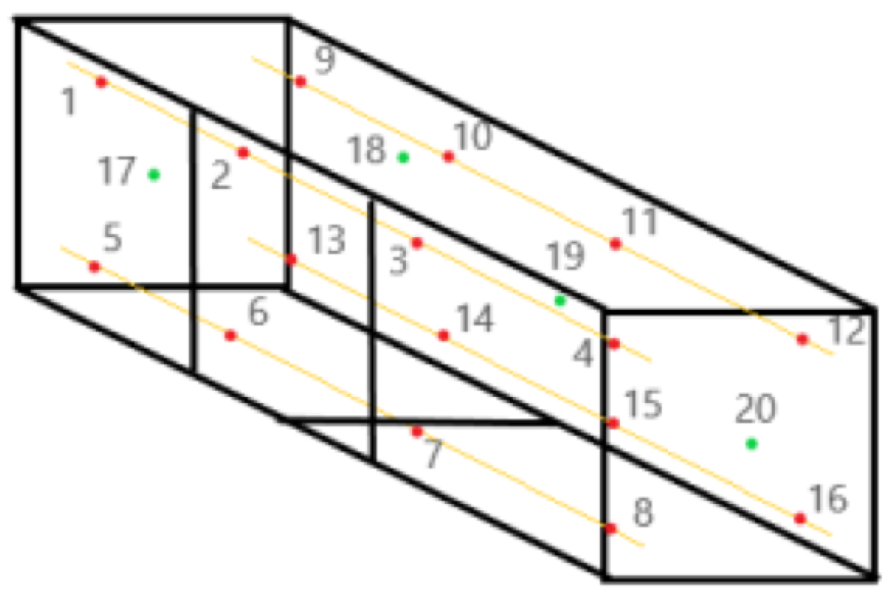
For temperature acquisition, a total of 20 copper T-type thermocouples (TC Direct, Madrid, Spain) with 0.2 mm wire were installed. Sixteen were installed inside the box as shown in
Figure 5 from 1 to 16, and the other four were installed outside marked from 17 to 20. The internal thermocouples were installed 100 mm from the panels by using four wires crossing the longest part of the enclosure. The external thermocouples were installed centered 250 mm from the face of the corresponding wall, the top, the back and the two side walls. The 20 thermocouples were connected to a data acquisition unit, DAQ970A by Keysight (Keysight, Santa Rosa, CA, USA), equipped with a 20 channels multiplexor (Keysight, Santa Rosa, CA, USA).
The transmittance is experimentally estimated with
where the electric power consumed
is given by the analyzer and the outer surface of the box is A =
. The experimental campaign consisted of seven experiments of 2 h of measurement each.
The thermal bridge is estimated with
where
.
5. Results and Discussion
Simulations for the first set, and corresponding semi-empirical estimation, have been performed with three different materials as insulators, with distinct thermal conductivities, as shown in
Table 3.
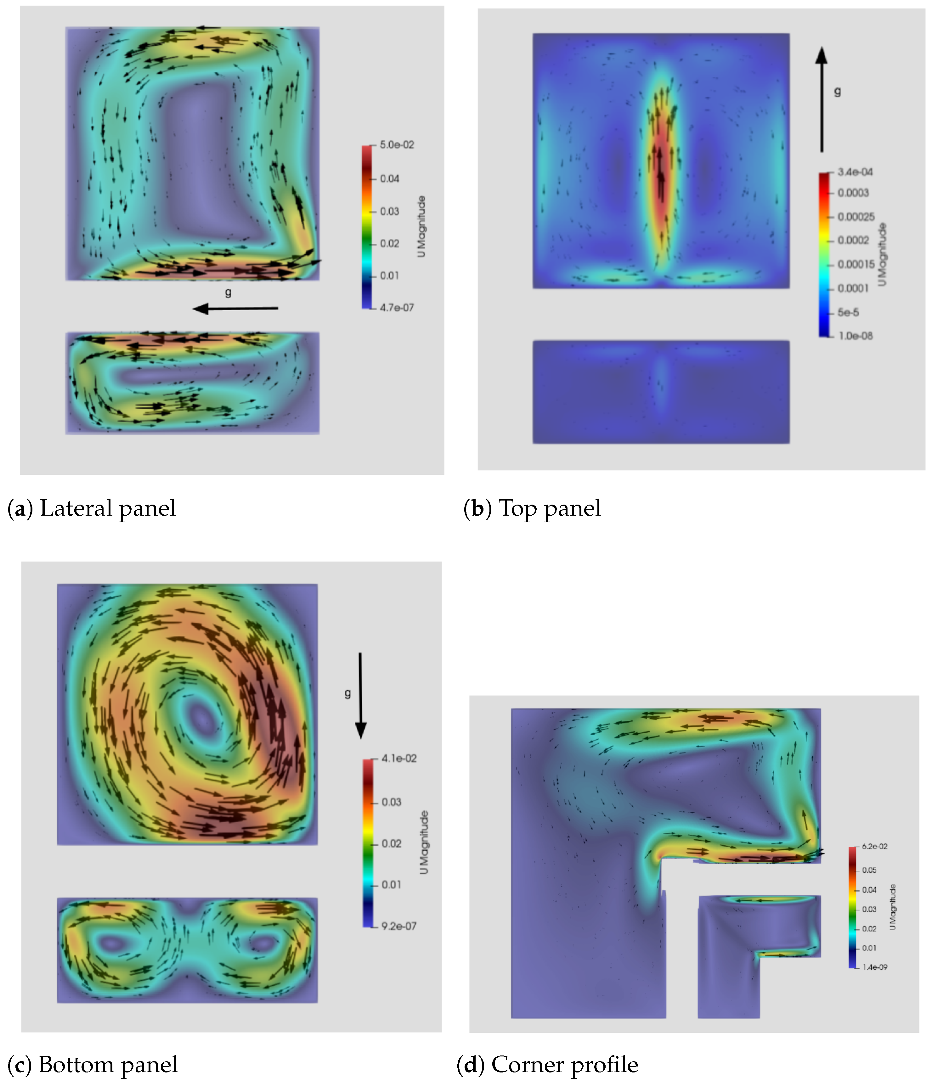
Figure 6 shows the velocity distribution for the Material 1, for the three orientations of the wall, vertical and horizontal downwards/upwards (note the orientation of gravity). For vertical wall and horizontal facing upwards the results of transmittance are comparable with an underestimation for semi-empirical approach of about 20% in the first case, and 13% in second case. In the case of horizontal wall facing downwards the disagreement is very strong between both approaches, being CFD computation almost four times smaller than semi-empirical estimation. This is due to the fact that in the numerical simulations forced convection could not be included due to the complexity of the boundary condition setup. This point has small influence for vertical and horizontal upwards walls, where natural convection dominates the heat transfer. But, in the case of horizontal downwards wall, gravity is in the opposite direction of the temperature gradient and it drastically reduces the heat transfer. Note that the velocity magnitude in
Figure 6b is of the order of less than 1 mm/s, whereas for vertical and upwards facing walls, it is about 50 mm/s.
The sections to be simulated will be those of the panels
Figure 6a–d.
With regard to the second kind of numerical simulations, a significant difference is observed between the numerical and semi-empirical results of the thermal transmittance without radiation, as shown in
Table 4, with a numerical value that is 67% higher than the semi-empirical one. This indicates that, in the absence of radiation, the numerical calculation produces a higher estimate of thermal transmittance compared to the semi-empirical approach. On the other hand, when considering the thermal bridge, the semi-empirical solution shows a slight superiority of about 2% compared to the numerical result.
A comparison between the experimental results and those obtained in the numerical simulation and semi-empirical estimation in the absence of radiation could not be undertaken, due to the impossibility of completely eliminating radiation in the experiments.
The results’ comparison among the three different methods with the global model with heat flux is shown in
Table 5.
When comparing the numerical results in the presence of radiation, significant differences are observed in relation to the experimental and semi-empirical results. In the case of thermal transmittance, the lowest estimate corresponds to the experimental results, while the numerical results are 8% higher. Semi-empirical estimation is 38% higher than the experimental results. Likewise, the semi-empirical estimate is 28% higher in relation to the numerical results. Regarding the thermal bridge factor, the highest estimation is the one obtained through the experiments, exceeding the numerical results by 3% and the semi-empirical approach by 8%.
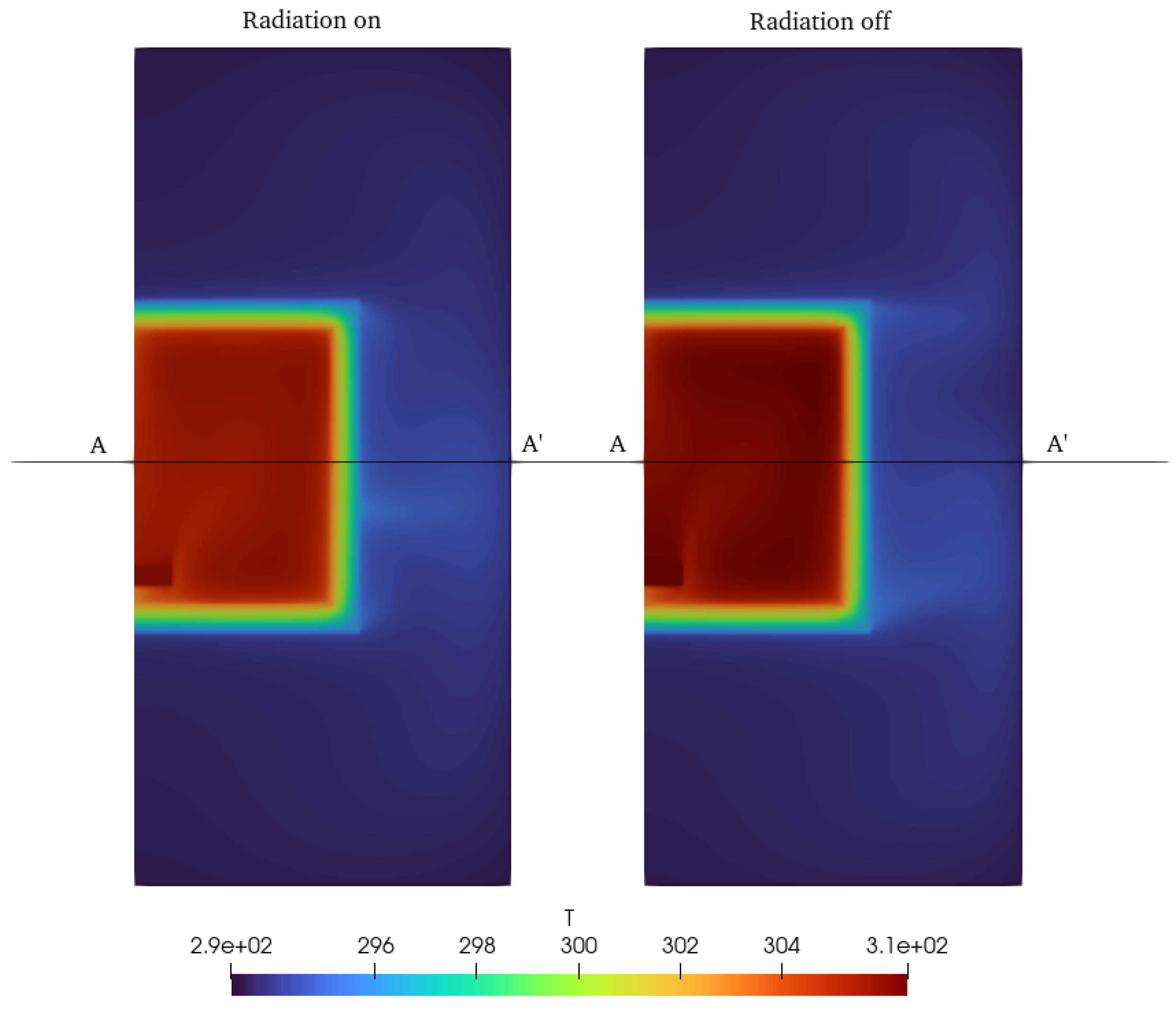
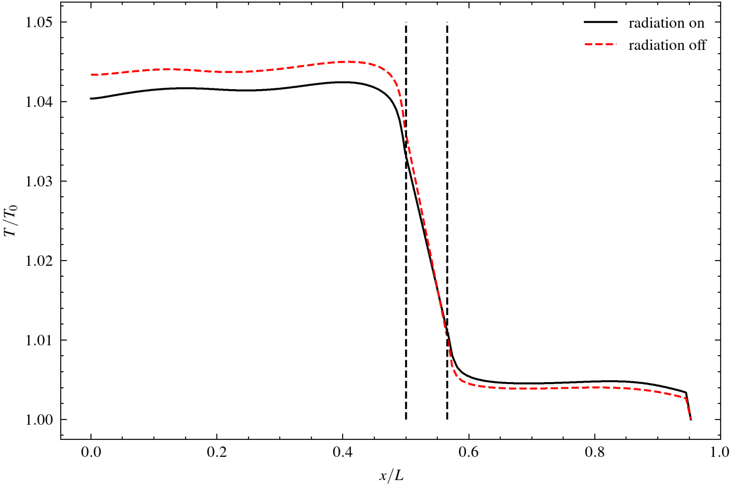
Figure 7 shows the distribution of velocity with the radiation term enabled and disabled. There is no appreciable difference of flow pattern inside the AHU and in the lower and upper parts of external air. In the lateral side, the vortex generated by the natural convection is displaced upwards in the case of radiation enabled. On the other side, when radiation is switched off the vortex seems to be slightly stronger and larger. This explains the difference of temperature distribution shown in
Figure 8 and
Figure 9. Temperature in the internal air is lower when radiation is considered due to the normal stream of air in the central part of the lateral panel that contributes to the heat evacuation by convection. These results suggest that radiation is an important term that has to be considered when the numerical computation of the heat transfer of an AHU is performed.
Results when radiation is activated in the global model are shown in the bar plot of
Figure 10. Numerical computation agrees very well with the experimental measurement with a value that is only 8% larger. The semi-empirical method, however, overestimates the value of
U in more than 38%. This disagreement between the semi-empirical and experimental results is compensated by the time and computational resources consumed. While CFD takes about a week with 8 parallel cores, the semi-empirical method performs the calculation in just a few seconds on a spreadsheet.
6. Conclusions
Semi-empirical estimation, experiments, and numerical simulations have been used to obtain accurate and clarifying results in the study of transmittance in air handling units. The combination of these three methods has led to more reliable results and a more complete understanding of transmittance in AHUs. This information is crucial for the efficient design and effective operation of air conditioning and ventilation systems (HVACs), as AHUs are key elements of HVACs, which in turn contribute to the improvement in energy efficiency and indoor air quality.
In general, it is observed that the semi-empirical results and the numerical simulations for the different sections of material 1 are quite similar where, in most cases, the numerical estimation is higher by up to 22%, depending on the case. This indicates a reasonable concordance between the two methods and suggests a fair accuracy in the semi-empirical estimation. On the other hand, the results for materials 2 and 3 are remarkably accurate as the difference between the results is 1% and 11%, respectively, indicating the high reliability of the numerical simulations.
Moreover, future work should focus on the refinement and improvement in the theoretical models and numerical simulations, taking into account additional factors such as the interaction between components, the variability of environmental conditions, and the inclusion of other relevant parameters. Furthermore, it is suggested that future research should focus on overcoming experimental limitations to obtain more reliable and comparable results, which will contribute to a more complete understanding of transmittance in AHUs and to the improvement in air-conditioning and ventilation systems.


 ,
, 


