Robust Data-Driven State of Health Estimation of Lithium-Ion Batteries Based on Reconstructed Signals

Abstract

The state of health (SoH) of lithium-ion batteries is critical for diagnosing the actual capacity of the battery. Data-driven methods have achieved impressive accuracy, but their sensitivity to sensor noise, missing samples, and outliers remains a limitation for their deployment. This paper proposes a robust, purely data-driven SoH estimation methodology that addresses these challenges. Our method uses a proposed non-iterative closed-form signal reconstruction derived from a modified Tikhonov regularization. Five new features were extracted from reconstructed voltage and temperature discharge profiles. Finally, a Huber regression model is trained using these features for SoH estimation. Six ageing scenarios built from the public NASA and Sandia National Laboratories datasets, under severe Gaussian noise conditions (10 dB SNR), were employed to validate our proposed approach. In noisy environments and with limited training data, our proposed approach maintains a competitive accuracy across all scenarios, achieving low error metrics, with an RMSE on the order of ${10}^{-4}$, an MAE on the order of ${10}^{-2}$, and a MAPE below 1%. It outperforms state-of-the-art deep neural networks, direct-feature Huber models, and hybrid physics/data-driven models. In this work, we demonstrate that robustness in SoH estimation for lithium-ion batteries is influenced by the choice of machine learning architecture, loss function, feature selection, and signal reconstruction technique. In addition, we found that tracking the time to minimum discharge voltage and the time to maximum discharge temperature can be used as effective features to estimate SoH in data-driven models, as they are directly correlated with capacity loss and a decrease in power output.

1. Introduction

Lithium-ion batteries (LIBs) are essential in the transition to sustainable energy systems [1]. They enable the storage of renewable energy for later use, which is critical for balancing supply and demand from intermittent energy sources [2]. In the electricity sector, LIBs are used for peak shaving, arbitrage, capacity firming, energy price management, frequency regulation, and grid stabilization [3]. Over time, batteries experience degradation due to multiple factors such as charge, discharge cycles, and the temperature effects of working conditions. State of health (SoH) estimation is important for assessing battery degradation of all the aforementioned applications and electric vehicles [4]. SoH is defined as the ratio of the actual capacity to the nominal capacity [5]. It is expressed as a percentage to diagnose the actual battery capacity [6]. For instance, a SoH below range of 70–80% indicates the end-of-life of the battery for primary applications since the battery can no longer deliver the required power density by high-performance storage systems [7]. However, such batteries can still be reused in second life applications (lower power applications) [8]. SoH estimation methods can be classified in the following four main categories [9]: (i) experimental methods, (ii) physics-based models, (iii) data-driven methods, and (iv) hybrid approaches [10].

Experimental methods, also known as direct measurement methods, include processes such as ampere-hour counting [11], which involves performing a full charge and discharge cycle between defined voltage thresholds. Specific current rates and temperature conditions are maintained during ampere-hour counting [9]. To determine the actual battery capacity Q, and SoH, the following formulation is employed:

$$\begin{array}{cc}\hfill & Q={\int }_0^{t_{\mathrm{f}}}\eta I\left(t\right)\mathrm{d}t\hfill \\ \hfill & SOH={\displaystyle \frac{Q}{Q_{\mathrm{initial}}}}\hfill \end{array}$$

(1)

where Q is the actual capacity, $Q_{\mathrm{initial}}$ is the initial capacity of a battery, $I\left(t\right)$ is the current, and $t_{\mathrm{f}}$ is the total time during charging or discharging. $\eta$ represents the coulombic efficiency, which is very close to 1 for LIBs [12]. However, these methods are time-consuming, require interrupting normal operation, and are limited to controlled laboratory environments [13].

Physics-based models [14] simulate the chemical and physical processes occurring within batteries. SoH is estimated by monitoring changes in some model parameters that are correlated with battery aging [15]. For instance, in equivalent circuit models (ECM) [16], LIBs are represented as electrical circuits with resistors, capacitors, and voltage sources [17]. As the battery ages, evidenced by a decline in SOH, the internal resistance parameter in ECM models increases, while the capacitance related to capacity tends to decrease [18]. Models calibrated under specific conditions may not apply directly to others, necessitating re-calibration across different operating scenarios [19].

Data-driven methods [20], such as machine learning (ML) algorithms, are trained on historical aging data (voltage, current, temperature, etc.) to identify complex patterns and relationships between the extracted features, e.g., health indicators and SoH [21]. Recent studies highlight that by using large datasets and carefully designed training settings, data-driven techniques can achieve high accuracy and adaptability in predicting battery SoH [22], often outperforming traditional physics-based models in terms of accuracy [22]. Therefore, data-driven methods are usually implemented in BMS to track degradation and estimate SoH [23]. However, SoH data-driven approaches often require large datasets for training [24] and are sensitive to noise and missing data [25]. Thus, selecting and extracting the right features for data-driven methods is non-trivial, especially with varying operating conditions and degradation mechanisms [26].

Hybrid approaches combine different sources of information and modeling techniques to enhance the accuracy, robustness, and interpretability of SoH estimation. For instance, physics-based models can be used to provide simulated features to data-driven approaches to perform SoH estimation with real and simulated data [27]. Recent studies have proposed knowledge transfer techniques; for instance, ref. [28] developed a transfer learning method that diagnoses degradation modes (DMs) of lithium–iron–phosphate (LFP) batteries by minimizing both classification loss and domain adaptation loss between synthetic and real datasets. This approach enables accurate DM identification without requiring extensive real-world labeled data. Similarly, ref. [29] proposed a two-stage SOH estimation framework where DM knowledge is first transferred from synthetic to real datasets and then used as input for SOH prediction.

In this work, we propose a novel pure data-driven SoH estimation approach of lithium-ion batteries, designed to demonstrate robustness against noisy measurements and outliers. Unlike previous methods, our proposed approach can be trained with small datasets. The proposed method does not need an explicit physics-based model or assumptions about initial aging conditions for maintaining high accuracy, making it suitable for real-time BMS implementation with low-computational cost and memory requirements. To highlight the advantages of the proposed methodology,

Table 1. Comparison of proposed SoH estimator with previous data-driven approaches.

Data-Driven Method	Number of Input Features	Robustness	Trainable Parameters	Performance Metric
Proposed Approach	5 proposed features based on signal reconstruction	Our proposed signal reconstruction approach can handle noise and outliers in the measurement data	6 polynomial parameters trained with Huber cost function	RMSE = ${10}^{-4}\%$, MAE = ${10}^{-2}\%$, MAPE = 1%
Deep Neural Network [31]	3 (Direct features)	The reported approach requires preparing the data by removing significant outliers manually	2 hidden layers with 30 and 15 neurons, respectively, as well as Sigmoid and Tanh activation functions	RMSE = 1.9 ×${10}^{-4}\%$, MAPE = 1.39%
Deep Neural Network [32]	6 (Direct features)	The paper does not discuss a dedicated noise handling mechanism	217 trainable parameters	RMSE = 0.004758%, MAE = 0.534%
Nonlinear Autoregressive Exogenous Neural Network [33]	8 (Model-based features)	The paper does not discuss a dedicated noise handling mechanism	Hidden neurons = 50, Feedback delays = 8	MAE = 0.72%, MaxE = 4.69%
Gated Recurrent Unit Network [34]	3 (Direct features)	Gaussian noise injection with a mean of 0 and a standard deviation of 1–2% into the voltage, current, and temperature measurements (works on less noise-corrupted signals)	Hidden neurons = 256 (GRU), convolution number = 64, size of each convolution layer 32 × 1	MAE = 1.03%, MaxE = 4.11%
Convolutional Neural Network [35]	1 (Preprocessed features)	The reported approach is sensitive to noise and outliers	Number of convolution kernels = 256, size of the kernel = 3 × 1	RMSE = 1.1%, MAE = 0.9%

presents a comparative analysis against previous data-driven and hybrid approaches that report the lowest error metrics for estimating lithium-ion battery state of health [30].

The summarized contributions of this paper are as follows:

• Closed-form signal reconstruction: We present a non-iterative closed-form solution for the signal reconstruction of noisy measurements.
• Novel data-driven health indicators: We introduce five noise-resilient features derived from the reconstructed voltage and temperature discharge profiles.
• Robust data-driven state of health estimation: In this work, we use the Huber cost function to improve the accuracy of the regression model by reducing the impact of outliers, providing an alternative to removing outliers from the dataset.

This paper is organized as follows: Section 1 introduces the SoH estimation problem for LIBs and reviews current modeling techniques in the literature. Section 2 outlines the proposed approach and the case studies. Section 3 presents a comprehensive performance assessment that demonstrates the effectiveness of our method compared to existing data-driven and hybrid methods in noisy environments and with limited training data. Finally, Section 4 concludes the paper, summarizing key findings and discussing potential directions for future work.

2. Materials and Methods

This section outlines the materials and methodology adopted in the development of the proposed SoH estimation approach for LIBs under noisy measurement conditions. As illustrated in Figure 1, the proposed method is described in detail in Section 2.1. This work assumed that there is an availability of data storage systems capable of continuously monitoring and recording voltage and temperature measurements from LIBs.

2.1. Proposed Approach

Our proposed approach consists of three key stages:

(1)

Signal Reconstruction: This stage estimates a vector ${\widehat{\mathbf{z}}}^m={\left({\widehat{z}}_1^m,{\widehat{z}}_2^m,\dots ,{\widehat{z}}_t^m\right)}^T$ from noisy voltage and temperature profiles ${\mathbf{z}}_c^m={\left(z_{c,1}^m,z_{c,2}^m\dots ,z_{c,t}^m\right)}^T$, where $m=1$ corresponds to the battery discharge voltage profile and $m=2$ represents the battery discharge temperature profile. The signal reconstruction employs the proposed closed-form, non-iterative mathematical expression formulated in Equation (8).

(2)

Feature Extraction: From the reconstructed voltage and temperature discharge profiles, five new data-driven health indicators are extracted, which are conditionally correlated with the battery aging process.

(3)

SoH Estimation: A Huber regression model was employed for SoH estimation, demonstrating robustness against outliers.

• Further details of each stage will be explained in the following sections.

2.1.1. Proposed Signal Reconstruction Stage

This subsection details the proposed signal reconstruction stage, designed to recover voltage and temperature discharge profiles from noisy measurement data. The measurement model employed in this work was formulated as follows:

$${\mathbf{z}}_c^m\triangleq {\mathbf{z}}^m+\mathbf{e}$$

(2)

where ${\mathbf{z}}^m$ represents the unknown noise-free signal for each discharge profile. The term $\mathbf{e}$ denotes the stochastic noise component affecting the measurements. The objective of the proposed signal reconstruction method is to estimate the clean signal, denoted as ${\widehat{\mathbf{z}}}^m$, from the noisy measurement ${\mathbf{z}}_c^m$. To achieve this, the signal reconstruction problem is formulated as a regularized optimization problem:

$$\underset{{\widehat{\mathbf{z}}}^m}{min}{∥{\widehat{\mathbf{z}}}^m-{\mathbf{z}}_c^m∥}_2^2+\delta \varphi \left(\Delta {\widehat{\mathbf{z}}}^m\right);$$

(3)

the regularization hyperparameter $\delta$ controls the trade-off between preserving the original noisy signal and noise filtering. The function $\varphi \left(\Delta {\widehat{\mathbf{z}}}^m\right)$ introduces a regularization term to improve robustness against measurement noise. When $\delta =0$, the reconstructed signal exactly matches the noisy measurement. Conversely, excessively high values of $\delta$ result in over-smoothing, potentially distorting the original signal characteristics. Two regularization strategies were investigated in this study: (i) Tikhonov regularization = $\varphi \left(\Delta {\widehat{\mathbf{z}}}^m\right)={∥\Delta {\widehat{\mathbf{z}}}^m∥}_2^2$ and (ii) LASSO regularization = $\varphi \left(\Delta {\widehat{\mathbf{z}}}^m\right)={∥\Delta {\widehat{\mathbf{z}}}^m∥}_1$.

To solve the ill-posed problem in Equation (3), the regularization hyperparameter $\delta$ is determined using the L-Curve method, as detailed in [36]. Additionally, we employ the regularization operator $\Delta$, previously reported in [36], and defined in Equation (4), due to its demonstrated stability in reconstructing voltage and temperature discharge profiles of lithium-ion batteries observed in this work.

$$\Delta =\left[\begin{array}{cccccccccc}\hfill 1& \hfill -1& \hfill 0& \hfill 0& \hfill 0& \hfill \cdots & \hfill 0& \hfill 0& \hfill 0& \hfill 0\\ \hfill -1& \hfill 2& \hfill -1& \hfill 0& \hfill 0& \hfill \cdots & \hfill 0& \hfill 0& \hfill 0& \hfill 0\\ \hfill 0& \hfill -1& \hfill 2& \hfill -1& \hfill 0& \hfill \cdots & \hfill 0& \hfill 0& \hfill 0& \hfill 0\\ \hfill 0& \hfill 0& \hfill -1& \hfill 2& \hfill -1& \hfill \cdots & \hfill 0& \hfill 0& \hfill 0& \hfill 0\\ \hfill ⋮& \hfill ⋮& \hfill ⋮& \hfill ⋮& \hfill ⋮& \hfill & \hfill ⋮& \hfill ⋮& \hfill ⋮& \hfill ⋮\\ \hfill 0& \hfill 0& \hfill 0& \hfill 0& \hfill 0& \hfill \cdots & \hfill -1& \hfill 2& \hfill -1& \hfill 0\\ \hfill 0& \hfill 0& \hfill 0& \hfill 0& \hfill 0& \hfill \cdots & \hfill 0& \hfill -1& \hfill 2& \hfill -1\\ \hfill 0& \hfill 0& \hfill 0& \hfill 0& \hfill 0& \hfill \cdots & \hfill 0& \hfill 0& \hfill -1& \hfill 1\end{array}\right]$$

(4)

where $\Delta \in {\mathbb{R}}^{t\times t}$ is a square matrix, with its dimension equal to the number of samples t in each discharge profile.

Signal Reconstruction Based on Tikhonov Regularization

The reconstruction of the signal is formulated based on a modified Tikhonov regularization strategy expressed in Equation (5). This formulation, known as the unrestricted form, allows us to obtain a non-iterative approach to recover clean discharge profiles from noisy measurements, as follows

$$\underset{{\widehat{\mathbf{z}}}^m}{min}{∥{\widehat{\mathbf{z}}}^m-{\mathbf{z}}_c^m∥}_2^2+\delta {∥\Delta {\widehat{\mathbf{z}}}^m∥}_2^2$$

(5)

This formulation can be rewritten in the following compact form:

$$\underset{{\widehat{\mathbf{z}}}^m}{min}{∥{\widehat{\mathbf{z}}}^m-{\mathbf{z}}_c^m∥}_2^2+\delta {∥\Delta {\widehat{\mathbf{z}}}^m∥}_2^2=\underset{{\widehat{\mathbf{z}}}^m}{min}{∥\left[\begin{array}{c}{\widehat{\mathbf{z}}}^m-{\mathbf{z}}_c^m\\ \sqrt{\delta }\Delta {\widehat{\mathbf{z}}}^m\end{array}\right]∥}_2^2$$

(6)

Equation (6) can be rewritten as

$$\underset{{\widehat{\mathbf{z}}}^m}{min}{∥\left[\begin{array}{c}{\widehat{\mathbf{z}}}^m-{\mathbf{z}}_c^m\\ \sqrt{\delta }\Delta {\widehat{\mathbf{z}}}^m\end{array}\right]∥}_2^2=\underset{{\widehat{\mathbf{z}}}^m}{min}{∥\left[\begin{array}{c}I\\ \sqrt{\delta }\Delta \end{array}\right]{\widehat{\mathbf{z}}}^m-\left[\begin{array}{c}{\mathbf{z}}_c^m\\ \mathbf{0}\end{array}\right]∥}_2^2$$

(7)

Solving for ${\widehat{\mathbf{z}}}^m$, the closed-form solution of signal reconstruction using modified Tikhonov regularization is given by

$${\widehat{\mathbf{z}}}^m={\left({\left[\begin{array}{cc}I& \\ \sqrt{\delta }\Delta \end{array}\right]}^T\left[\begin{array}{cc}I& \\ \sqrt{\delta }\Delta \end{array}\right]\right)}^{-1}{\left[\begin{array}{cc}I& \\ \sqrt{\delta }\Delta \end{array}\right]}^T\left[\begin{array}{c}{\mathbf{z}}_c^m\\ 0\end{array}\right]$$

(8)

Signal Reconstruction Based on LASSO Regularization

In the case of LASSO regularization strategy, it is not possible to have a closed-form expression. However, the ill-posed problem can be effectively solved using the following constrained optimization problem.

$$\begin{array}{cc}\hfill min\hfill & \delta {\parallel \Delta {\widehat{\mathbf{z}}}^m\parallel }_1\hfill \\ \hfill \mathrm{s}.\mathrm{t}.\hfill & {∥{\widehat{\mathbf{z}}}^m-{\mathbf{z}}_c^m∥}_2^2\le \delta \hfill \end{array}$$

(9)

For this study, the regularization parameter $\delta$ was empirically set to 5 for signals with a signal-to-noise ratio (SNR) of 10 dB. The optimal choice of $\delta$ is inherently dependent on the noise characteristics of the data:

• For highly corrupted signals (SNR < 10 dB), larger $\delta$ values ($\delta >5$) are recommended to enhance noise suppression.
• For signals with minimal noise contamination (SNR > 10 dB), lower $\delta$ values ($\delta <5$) preserve original signal details.

2.1.2. Proposed Feature Extraction Stage

We propose a systematic approach to extract features highly correlated with battery health degradation by analyzing the evolving patterns in voltage and temperature profiles during discharge cycles. The method consists of three steps:

• Identification of discharge cycle.
• Extraction of voltage features.
• Extraction of temperature features.

1. Identification of discharge cycle: We isolate the continuous discharge cycles from battery operation data by identifying periods where the current drops below a predefined threshold (in this case −0.05 A) and where a predefined minimum voltage (e.g., cutoff voltage) is reached. Note that manufacturers generally set a safe cutoff voltage to preserve battery health and lifespan [37]. Lower cutoff voltages (e.g., 2.0 V) correspond to a depth of discharge (DOD) closer to 100%. However, in real-time applications, battery manufacturers generally do not recommend a 100% DOD as an operational norm [38]. Many battery studies suggest limiting the DOD to 70% to extend battery lifespan [39]. This step ensures we analyze only discharge events, filtering out partial or interrupted discharge cycles that could skew the analysis.

2. Extraction of voltage features: Battery voltage during discharge follows a decreasing pattern, where each successive voltage measurement is lower than the previous one, ${\widehat{z}}_1^1>{\widehat{z}}_2^1>\dots >{\widehat{z}}_t^1$, and whose characteristics change as the battery degrades. We capture these dynamics through two critical features:

• Minimum discharge voltage ($x_1$): This is the lowest voltage reached during the discharge cycle (cutoff voltage). As a battery ages, its internal impedance increases due to factors such as lithium inventory loss and conductive degradation [40]. An increment in the impedance leads to a more pronounced voltage drop ($R_{0}i$) during discharge [41]. According to the Shepherd model, the terminal voltage V at discharge time t can be modeled as follows [42]:   

  $$V\left(t\right)=E_0-K\left[{\displaystyle \frac{Q}{Q-i\left(t\right)\times t}}\right]i\left(t\right)-R_{0}i\left(t\right)$$

  (10)

  where $E_0$ is the theoretical initial open-circuit voltage under specific working conditions, $R_0$ represents the internal ohmic resistance of the battery $(\Omega )$, i is the discharge current in amperes (A), assumed positive, and Q is the actual full capacity of the battery in ampere-hours ($Ahr$), in which eventually, with aging, its experiment capacity will fade. $Q-i\left(t\right)\times t$ is the remaining capacity in the battery at discharge time t and K is the polarization resistance coefficient $(\Omega )$. Thus, the minimum discharge voltage is sensitive to internal resistance growth, and to the battery’s full capacity Q. In this work, we found that tracking the time to minimum discharge voltage can be used as a feature to estimate SoH in data-driven models.
• Time to minimum voltage ($x_2$): This is the duration between the beginning of discharge and the minimum voltage. A healthy battery with full capacity can sustain the discharge current longer before reaching the voltage limit, whereas an aged battery with capacity fade will hit the minimum voltage sooner [43].

3. Extraction of temperature features: Temperature profiles during discharge typically exhibit an increasing pattern, where each successive temperature reading surpasses the previous one, ${\widehat{z}}_1^2<{\widehat{z}}_2^2<\dots <{\widehat{z}}_t^2$, and which changes with battery aging. To capture these thermal characteristics, we introduce three temperature-related features:

• Minimum temperature at the beginning of discharge ($x_3$): The baseline temperature at the beginning of discharge, establishing a reference point.
• Maximum discharge temperature ($x_4$): The peak temperature reached during discharge, reflecting internal resistance and exothermic reactions. As the battery degrades and its internal resistance increases, it produces more heat for the same discharge current, resulting in a higher peak temperature [44].
• Time elapsed between minimum and maximum temperature ($x_5$): The aged battery’s temperature climbs to its maximum in a shorter time than in a new battery, which heats more slowly due to its lower internal resistance [45].

These proposed features effectively encapsulate the electrochemical and thermal signatures of battery degradation without requiring complete charge–discharge curves. All extracted features ${\mathbf{x}}_i$ were normalized to lie between 0 and 1 to ensure numerical stability and consistency.

2.1.3. State of Health (SoH) Estimation

SoH is estimated using a Huber regression model (Equation (11)), a robust method less sensitive to outliers than least squares regression [46]. The Huber loss function [46] (Equation (12)) is used to fit the model, which smoothly transitions from a quadratic form for small residuals to a linear form for large residuals. This adaptive property mitigates the influence of outliers while maintaining sensitivity to minor deviations [46], making it particularly well-suited for SoH estimation of noisy data.

$$\widehat{y}={\alpha }_0+{\alpha }_1{x}_1+{\alpha }_2{x}_2+{\alpha }_3{x}_3+{\alpha }_4{x}_4+{\alpha }_5{x}_5$$

(11)

where the $\alpha$ coefficients are optimized by solving a convex quadratic programming problem [47] and $x_i$ represents our proposed features. We set the Huber transition parameter to $\gamma =1.35$, which yields approximately 95% efficiency under Gaussian noise. This choice promotes numerical stability by limiting the influence of extreme residuals, thereby helping to prevent overfitting even in high-dimensional feature spaces. The Huber cost function [48], used in the training stage to fit the model, is defined as follows:   

$$L_{\gamma }(y_i,{\widehat{y}}_i)=\left\{\begin{array}{cc}{\displaystyle \frac{1}{2}}{(y_i-{\widehat{y}}_i)}^2\hfill & \mathrm{for} |y_i-{\widehat{y}}_i| \le \gamma ,\hfill \\ \gamma |y_i-{\widehat{y}}_i|-{\displaystyle \frac{1}{2}}{\gamma }^2\hfill & \mathrm{otherwise}.\hfill \end{array}\right.$$

(12)

Once trained, the Huber regression model provides accurate SoH estimates, $\widehat{y}$, from the five extracted features. As shown in Figure 1, incorporating Huber regression into our pipeline ensures computational efficiency and robustness against outliers.

Training and testing were performed using labeled datasets, which are described comprehensively in Section 2.2.

2.2. Datasets

The proposed SoH estimation method was evaluated using two distinct datasets: the NASA battery dataset [49] and Sandia National Laboratories (SNL) battery degradation dataset [50].

2.2.1. NASA Data Overview

To evaluate our proposed SoH estimation method, experiments were performed using three distinct testing scenarios derived from NASA’s lithium-ion battery aging dataset [49]. The selected batteries and scenarios ensure various realistic operational scenarios, including temperature variations, different discharge cutoff voltages, diverse capacity fade thresholds, and the end-of-life (EOL) criteria.

Scenario 1: Variable Temperature Conditions. In this scenario, we evaluate our proposed SoH estimation method over a broad temperature range from 4 °C to 40 °C. Batteries B0005 and B0007 were used for model training, while Battery B0018 was reserved exclusively for testing purposes. The charging protocol consisted of a constant current (CC) phase at 1.5 A until the battery voltage reached 4.2 V, then a constant voltage (CV) phase was maintained at 4.2 V until the charging current decreased to 20 mA. The discharge cutoff voltages varied across the batteries, set at 2.7 V for B0005, 2.2 V for B0007, and 2.5 V for B0018. The end-of-life criterion was determined based on a capacity fade of 30%, corresponding to a decrease from the nominal capacity of 2.0 Ah to 1.4 Ah.

Scenario 2: Constant Temperature Conditions. In Scenario 2, the batteries operated under controlled ambient conditions, with a constant temperature of 24 °C. Battery B0033 was used for training purposes, while B0034 was reserved for testing. The charging protocol was identical to Scenario 1, with the difference that the discharge cutoff voltages were set at 2.0 V for B0033 and 2.2 V for B0034. A more demanding end-of-life criterion was adopted, defined by a capacity fade threshold of 20%, also corresponding to a reduction in battery capacity from the initial 2.0 Ah to 1.6 Ah.

Scenario 3: Low-Temperature Operation: In this scenario, the batteries operated under low-temperature conditions (4 °C). The charging protocol followed the previously established procedure, with the difference that the discharge cutoff voltages among batteries were set at the following: 2.2 V for B0046, 2.5 V for B0047, and 2.7 V for B0048. The end-of-life criterion was the same as Scenario 1, defined as a 30% capacity fade.

Using the aforementioned scenarios, we evaluate the proposed SoH estimation method under different working conditions, as described in [51] and shown in

Table 2. Operating parameters of batteries from NASA dataset.

Battery ID	End Voltage (V)	Ambient Temperature (°C)	Nominal Capacity (Ah)	Discharge Current (A)	End of Life Criteria (Ah)	No. of Cycles
B0005	2.7	4 to 40	2	2	1.4	168
B0007	2.2	4 to 40	2	2	1.4	168
B0018	2.5	4 to 40	2	2	1.4	132
B0033	2.0	24	2	4	1.6	198
B0034	2.2	24	2	4	1.6	198
B0046	2.2	4	2	1	1.4	72
B0047	2.5	4	2	1	1.4	72
B0048	2.7	4	2	1	1.4	72

.

2.2.2. SNL Data Overview

We also evaluated our proposed SoH estimation method using three additional testing scenarios derived from the Sandia National Laboratories (SNL) lithium-ion battery aging dataset [50]. SNL’s dataset contains detailed cycle-level and time-series battery performance data collected during charge–discharge cycling tests on commercial 18650-format lithium–iron–phosphate (LFP) cells. Each battery was subjected to varied experimental conditions, including temperature, charge–discharge current rates, and state-of-charge (SoC) ranges. The data were acquired through the open-access web platform [52].

Scenario 4: High-stress regime. In this scenario, both training and test datasets from lithium–iron–phosphate (LFP) 18650 cells were cycled at 25 °C ambient temperature. Cells were charged at a rate of 0.5C and discharged at a rate of 1C (where C represents the battery’s capacity in ampere-hours (Ah)), covering a full SoC range from 0% to 100% (complete depth of discharge). Specifically, the training data originated from the file SNL_18650_LFP_25C_0-100_0.5-1C_c_timeseries.csv, while testing data were taken from SNL_18650_LFP_25C_0-100_0.5-1C_d_timeseries.csv. Discharge rate conditions varied between 0.5C and 2C.

Scenario 5: Higher discharge rate. The training dataset was obtained from the file SNL_18650_LFP_15C _0-100_0.5-2C_a_timeseries.csv, while the testing dataset was sourced from SNL_18650_LFP_15C_0-100_0.5-2C_b_timeseries.csv. Compared to other scenarios, Scenario 5 is characterized by its lower operating temperature conditions (15 °C) and a higher discharge rate (2C), resulting in shorter discharge durations at high voltage per cycle.

Scenario 6: High-stress regime. The working conditions of this scenario are similar to those of Scenario 4, but with different batteries. For the training data, we used the file SNL_18650_LFP_25C_0-100_0.5-1C_a_timeseries.csv, while the data used for testing were taken from the file SNL_18650_LFP_25C_0-100_0.5-1C_b_timeseries.csv.

The proposed SoH estimation methodology was evaluated across the aforementioned defined scenarios, detailed in

Table 3. Operating parameters of batteries from SNL dataset.

	Cathode Chemistry
	NCA	NMC
Manufacturer	Panasonic	LG Chem
Manufacturer City—Country	Osaka—Japan	Seoul—Republic of Korea
Manufacturer PN	NCR18650B	18650HG2
Battery type	18650	18650
Nominal capacity [Ah]	3.2	3
Nominal voltage [V]	3.6	3.6
Voltage range [V]	2.5–4.2	2.0–4.2
Max discharge current [A]	6	20
Temperature range [°C]	0–45	−5–50
Charge C-rate	0.5C	0.5C
Discharge C-rate	0.5C/1C/2C	0.5C/1C/2C
Test temperature [°C]	15/25/35	15/25/35
Depth of discharge	0–100%	0–100%

. Note, NCA means Lithium Nickel Cobalt Aluminum Oxide, and NMC means Lithium Nickel Manganese Cobalt Oxide. Hence, NCA and NMC refer to two different types of lithium-ion battery cathode chemistries.

2.3. Accuracy Evaluation Metrics

A robust SoH estimation model maintains its accuracy across a wide range of scenarios. To evaluate the accuracy of our proposed SoH estimation methodology, three widely used evaluation metrics [53] were employed: mean absolute percentage error (MAPE), mean absolute error (MAE), and root mean square error (RMSE). These metrics provide complementary measures of estimation accuracy, as detailed below:

• Mean Absolute Percentage Error (MAPE) quantifies the relative error as a percentage, making it easy to interpret and compare across different datasets or models, and is defined as follows:

  $$\mathrm{MAPE}={\displaystyle \frac{1}{n}}\sum _{i=1}^n\left|{\displaystyle \frac{{\widehat{y}}_i-y_i}{y_i}}\right|$$

  (13)
  Note that MAPE can be misleading when actual $y_i$ values are close to zero, as the percentage error becomes disproportionately large.
• Mean Absolute Error (MAE) measures the average magnitude of absolute deviations between the estimated and actual SoH values. Lower MAE values indicate higher prediction accuracy. Mathematically, it is expressed as follows:

  $$\mathrm{MAE}={\displaystyle \frac{1}{n}}\sum _{i=1}^n\left|{\widehat{y}}_i-y_i\right|$$

  (14)
  Note that MAE is less sensitive to outliers compared to metrics like Root Mean Squared Error (RMSE), as it does not square the error.
• Root Mean Square Error (RMSE) evaluates the standard deviation of prediction errors, heavily penalizing large deviations. RMSE is computed as follows:

  $$\mathrm{RMSE}=\sqrt{{\displaystyle \frac{1}{n}}\sum _{i=1}^n{\left({\widehat{y}}_i-y_i\right)}^2}$$

  (15)

  Note that RMSE is sensitive to outliers.
  where ${\widehat{y}}_i$ is the estimated SoH, $y_i$ is the ground truth SoH, and n is the total number of SoH observations.

3. Numerical Results and Discussion

We first describe the experimental setup in Section 3.1, then provide a comprehensive experimental validation and performance analysis of our SoH estimation methodology under various noise levels, charging protocols, and operational conditions.

3.1. Experimental Setup

Our proposed SoH estimation method was evaluated using the scenarios detailed in Section 2.2. All experiments were conducted on a workstation assembled in Dell’s manufacturing facility located in Hortolândia, São Paulo, Brazil, with an Intel(R) Core(TM) i7 870 processor and 8 GB RAM. The proposed approach presented in Section 2.1 was implemented in Python 3.8 [54].

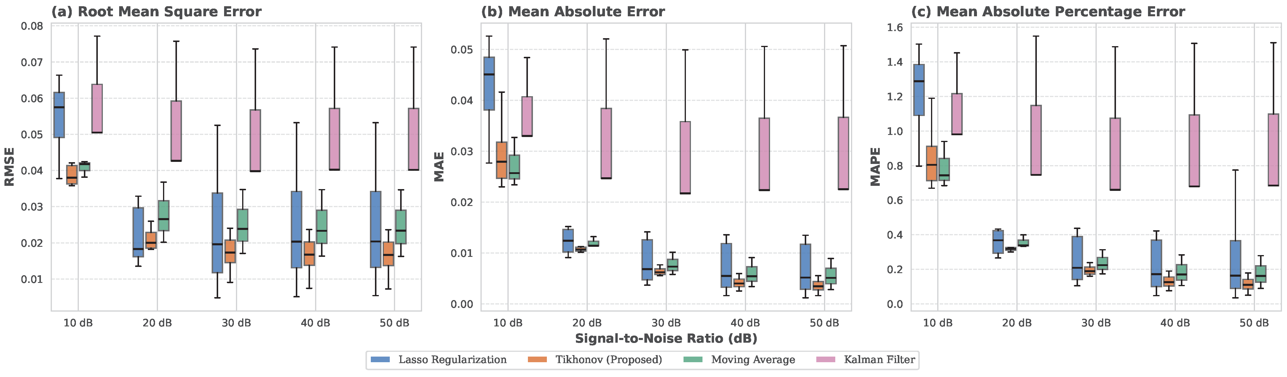
3.2. Sensitivity Analysis of Signal Reconstruction

The voltage and temperature discharge profile data for each scenario, detailed in Section 2.2, were distorted according to the following signal-to-noise ratio (SNR) ranges: 10, 20, 30, 40, 50 dB. All signals were normalized to zero mean and unit variance before processing to ensure a fair comparison across methods and parameter values. For each SNR level, we identified the optimal regularization parameter $\delta$ for both Lasso and Tikhonov methods using grid search. Our proposed approach assumes that sensor noise follows a zero-mean Gaussian distribution. This is a common characteristic of real-world sensor data according to [55]. Both our proposed approach based on modified Tikhonov formulation (Equation (8)) and LASSO formulation (Equation (9)) demonstrated stable performance under noisy conditions. However, our proposed approach achieves the lowest error metrics across multiple SNR levels, outperforming filtering methods such as moving average (MA) [56] and Kalman filter [57] for signal reconstruction, as shown in Figure 2.

In contrast to our proposed closed-form solution, which provides stable reconstructions for ill-posed inverse problems, LASSO formulation requires an iterative solution process and can be sensitive to convergence criteria and regularization parameter tuning. Therefore, we found that the LASSO formulation has a higher error variability than our proposed approach based on modified Tikhonov. On the other hand, the moving average (MA) filter operates by smoothing data points over a specified window. However, MA can lead to oversmoothing and the loss of important features in the signal, particularly in the presence of sharp transitions or edges. We found that this characteristic often results in insufficient performance when the signal reconstruction involves non-stationary or rapidly changing signals. In contrast, our proposed approach promotes piecewise constant solutions that are beneficial for reconstructing signals with abrupt changes. Thus, our proposed signal reconstruction method not only reduces noise effectively but also preserves essential signal characteristics that simple averaging methods can overlook. In this study, the centered MA filter [56] was implemented using Equation (16)

$$y\left[n\right]={\displaystyle \frac{1}{M}}\sum _{i=0}^{M-1}x\left[n+i-{\displaystyle \frac{M-1}{2}}\right]$$

(16)

where M represents the predefined samples (window size) that are used to average the original input signal $x\left[n\right]$ and n is the time index. In this work, we use $M=5$ obtained from a grid search. This allows the filter to process both past and future samples in a symmetric manner.

Kalman filter addresses the signal reconstruction problem by forming a recursive estimation procedure that integrates predictions based on the following dynamic model [57]:

$$x_k=x_{k-1}+w_k,w_k\sim \mathcal{N}(0,Q),$$

(17)

where $x_k\in \mathbb{R}$ is the latent (noise-free) signal sample at discrete time step k and $Q>0$ is the process-noise variance that captures unmodeled perturbations and model mismatch. Each noisy observation $z_k$ was modeled with direct noisy measurement $v_k$, as follows:

$$z_k=x_k+v_k,v_k\sim \mathcal{N}(0,R),$$

(18)

where $R>0$ is the measurement-noise variance. Our proposed approach based on Tikhonov formulation uses all data (e.g., all discharge voltage and temperature profiles) in a single batch. In contrast, the Kalman filter performs a sequential filtering by updating the reconstruction solution at each sample k. The Kalman filter achieves optimality only when $(Q,R)$ match the true process and sensor variances. Hence, we found that our proposed method is more robust to non-optimal hyperparameter specification compared with the Kalman filter. The experimental results demonstrate that our proposed approach achieves lower bias and variance than the Kalman filter for the signal reconstruction task under varying noise levels. This highlights the importance of sufficient data information for accurate reconstruction, providing stability against noise. Figure 2 is organized as follows: the boxplots show the RMSE, MAE, and MAPE for all the estimated SoH across different SNRs. SNR quantifies the measurement error for each measurement using (19).

$${\mathrm{SNR}}_{\left[\mathrm{dB}\right]}=10{log}_{10}{\displaystyle \frac{\mathbb{E}\left[z^2\right]}{{\sigma }_z^2}}$$

(19)

The error $\mathbf{e}\stackrel{\mathrm{iid}}{\sim }\mathcal{N}\left(0,{\sigma }_z^2\right)$ is used to pollute each measurement ${\mathbf{z}}_c^m$ in Equation (2). Signal reconstruction is an ill-conditioned problem, which can lead to convergence issues. To mitigate this, we introduced a closed-form solution in Equation (8) that ensures reliable performance even when the LASSO formulation encounters convergence difficulties. To do this, it is required to use the proposed regularization operator presented in Equation (4), which was introduced in a previous paper by our research group [36]. Since the proposed closed-form expression is a non-iterative mathematical model, the number of iterations required to obtain a signal reconstruction solution is one. Consequently, a significant reduction in computational time is observed.

Table 4. Comparison of signal reconstruction accuracy for the proposed closed-form Tikhonov, the iterative LASSO formulation, a centred moving-average (MA) filter, and a recursive Kalman filter under five noise conditions (SNR = 10–50 dB). Lower values of RMSE, MAE, and MAPE indicate superior reconstruction quality. The best results in each column are in bold.

Metrics	Method	SNR (dB)					Average
		10	20	30	40	50
RMSE	Tikhonov	0.0404	0.0210	0.0172	0.0165	0.0164	0.0223
	MA	0.0408	0.0278	0.0252	0.0248	0.0248	0.0287
	Lasso	0.0547	0.0248	0.0240	0.0247	0.0248	0.0306
	Kalman	0.0594	0.0537	0.0511	0.0515	0.0515	0.0534
MAE	Tikhonov	0.0295	0.0112	0.0064	0.0041	0.0035	0.0109
	MA	0.0273	0.0120	0.0077	0.0060	0.0056	0.0117
	Lasso	0.0427	0.0144	0.0104	0.0091	0.0088	0.0171
	Kalman	0.0381	0.0338	0.0311	0.0318	0.0319	0.0334
MAPE (%)	Tikhonov	0.8497	0.3295	0.1940	0.1299	0.1133	0.3233
	MA	0.7894	0.3566	0.2369	0.1866	0.1764	0.3492
	Lasso	1.2197	0.4241	0.3164	0.2809	0.2719	0.5026
	Kalman	1.1377	1.0139	0.9360	0.9553	0.9601	1.0006

shows the reduction in reconstruction signal quality as noise levels increase. However, our proposed approach maintains a consistent good performance in terms of accuracy. These findings support the selection of our proposed modified Tikhonov reconstruction stage within the proposed SoH estimation method.

3.3. Sensitivity and Correlation Analysis of Proposed Features

It is necessary to understand the importance of each feature for SoH estimation and provide insights into model goodness-of-fit in relative terms; that is, not merely whether the model performs well, but which features contribute most to its performance. To do this, we conducted a sensitivity analysis of the proposed features shown in

Table 5. Sensitivity analysis of proposed features. Checkmark (✓) indicates inclusion and a dash (-) indicates exclusion of the corresponding proposed features: minimum discharge voltage ($x_1$), time to minimum voltage ($x_2$), minimum temperature at the start of discharge ($x_3$), maximum discharge temperature ($x_4$), and time elapsed between minimum and maximum temperature ($x_5$). The best results are in bold.

Proposed Features					RMSE	MAE	MAPE (%)	R2	Time (s)
x1	x2	x3	x4	x5
✓	✓	✓	✓	✓	0.0862	0.0732	0.5987	0.923523	0.0259
-	✓	✓	✓	✓	0.233401	0.1855705	1.2169	0.913716	0.01905
✓	-	✓	✓	✓	1.0651395	0.8038405	2.60585	0.628143	0.0176
✓	✓	-	✓	✓	0.2290405	0.181089	0.70005	0.922905	0.01785
✓	✓	✓	-	✓	0.230986	0.18282	0.64605	0.9241995	0.01835
✓	✓	✓	✓	-	0.2297205	0.181146	0.73265	0.923476	0.01975
✓	-	-	-	-	1.393372	1.171515	8.9394	−1.454	0.0076
-	✓	-	-	-	0.231793	0.1860235	1.22655	0.9275805	0.0086
-	-	✓	-	-	1.1681775	0.862342	4.66665	0.08354	0.0079
-	-	-	✓	-	1.1566025	0.8757905	6.4991	−0.63832	0.0067
-	-	-	-	✓	1.364249	1.157678	3.33345	0.4079215	0.00895

. In this analysis, we examined model performance under different feature combinations: using all features, leaving one feature out, and using only a single feature. We evaluated each combination using error metrics (RMSE, MAE, MAPE), the coefficient of determination ($R^2$), and execution time. Note that $R^2$ quantifies the proportion of variance in the SoH variable that is estimated from one or more features, defined as

$$R^2=1-{\displaystyle \frac{{\sum }_{i=1}^n{\left(y_i-\widehat{y}i\right)}^2}{{\sum }_{i=1}^n{\left(y_i-\overline{y}\right)}^2}}$$

(20)

where $\overline{y}$ is the mean of the true values. In this formulation, $R^2=1$ indicates a perfect fit of the model to the data, corresponding to zero residual error (${\sum }_{i=1}^N{\left(y_i-\widehat{y}i\right)}^2=0$), whereas $R^2=0$ indicates that the model is no better than predicting the mean of the data (${\sum }_{i=1}^N{\left(y_i-\widehat{y}i\right)}^2={\sum }_{i=1}^N{\left(y_i-\overline{y}\right)}^2$). Thus, $R^2=0.90$ means that 90% of the variance in SoH is explained by the model. It is worth noting that $R^2$ can be negative if the model’s predictions are worse than simply using the mean $\overline{y}$, although in a well-trained regression for SoH we expect $R^2$ to be between 0 and 1.

We use the Pearson correlation coefficient to measure the degree of linear correlation between our proposed features and the SoH, based on the following formulation

$$r={\displaystyle \frac{{\sum }_{i=1}^n\left(x_i-\overline{x}\right)\left(y_i-\overline{y}\right)}{\sqrt{{\sum }_{i=1}^n{\left(x_i-\overline{x}\right)}^2{\sum }_{i=1}^n{\left(y_i-\overline{y}\right)}^2}}}$$

(21)

where $x_i$ indicates the proposed features and $y_i$ the SoH, and ${\overline{x}}_i$ and ${\overline{y}}_i$ are their average values, respectively. The range of the Pearson correlation coefficient is $[-1,1]$. The closer to the extreme values at both ends, the stronger the linear correlation between the proposed features and SoH. For detailed information of the correlation analysis, see

Table 6. Pearson correlation coefficients (r) between each of the five proposed features and the battery state of health (SoH), reported separately for the training set, the independent test set, and the combined dataset. The strong positive correlations of the temporal features $x_2$ and $x_5$ with SoH corroborate their dominant explanatory power, whereas $x_1$, $x_3$, and $x_4$ show only weak or moderate association. A negative sign indicates an inverse monotonic relationship with SoH.

Proposed Features	Train	Test	Overall
$x_1$: minimum discharge voltage	−0.1465	−0.2116	−0.1791
$x_2$: time to minimum voltage	0.9689	0.9627	0.9658
$x_3$: minimum temperature at the start of discharge	−0.0340	0.2752	0.1206
$x_4$: maximum discharge temperature	0.0357	−0.0601	−0.0122
$x_5$: time elapsed between minimum and maximum temperature	0.9625	0.9305	0.9465

.

Based on Table 6, we found that tracking the time to minimum discharge voltage and the time to maximum discharge temperature can be used as effective features to estimate SoH in data-driven models, as they are directly correlated with capacity loss and a decrease in power output.

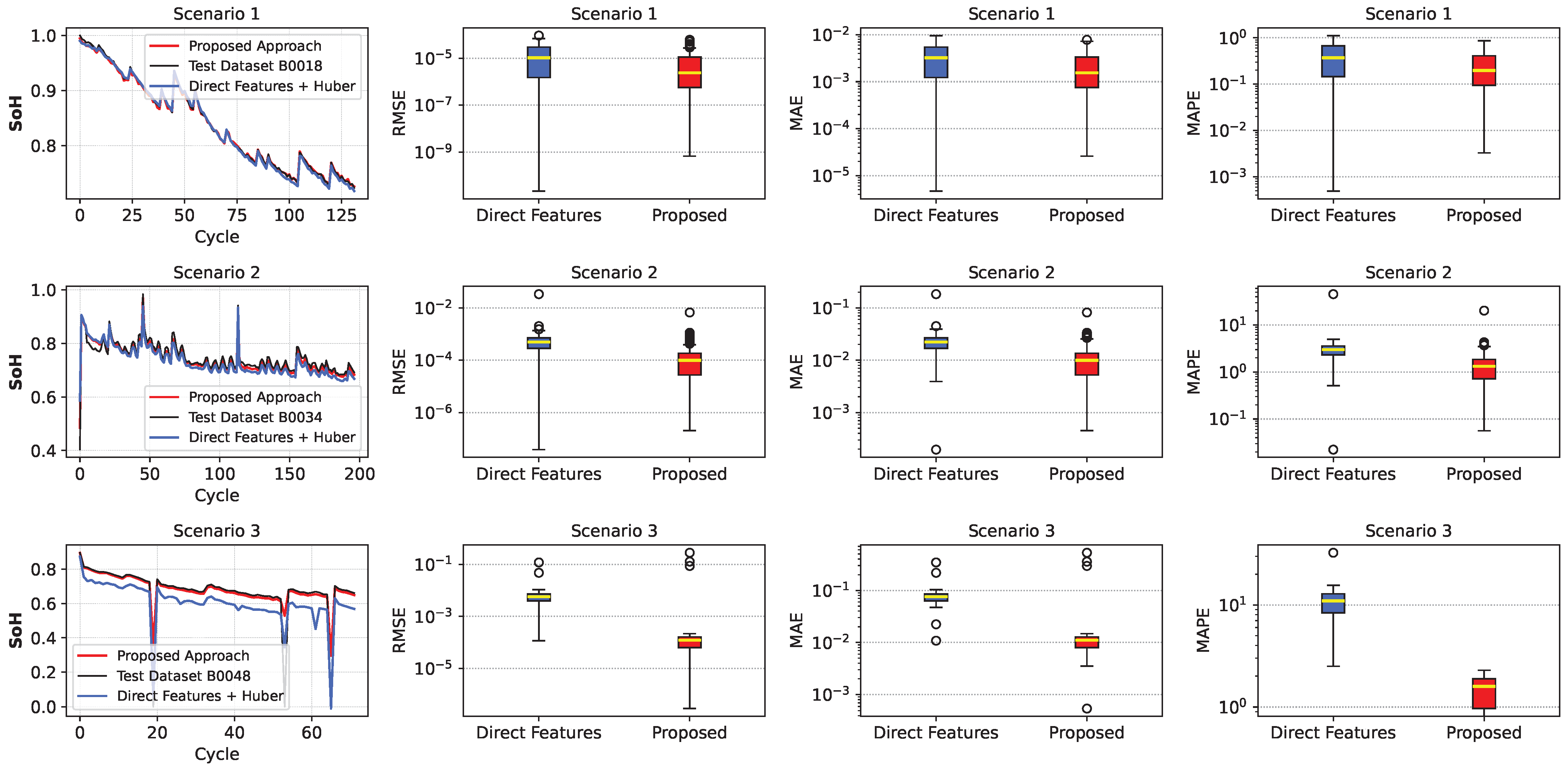
3.4. Comparison of Feature Selection: Direct Features vs Proposed

We compared our proposed five features, detailed in Section 2.1.2, with the direct features approach reported in [58], which uses the following ten features: minimum, maximum, and average values of voltage, current, temperature, and the total discharge time. Both methods use Huber regression, which is robust to outliers, along with the proposed signal reconstruction stage, differing only in their features. As depicted in Figure 3, our proposed method outperformed the direct features method in terms of accuracy across different battery-aging scenarios. Our proposed features, despite using fewer features than direct features [58], perform better, showing that our proposed feature engineering is more effective than just collecting a wide range of statistics.

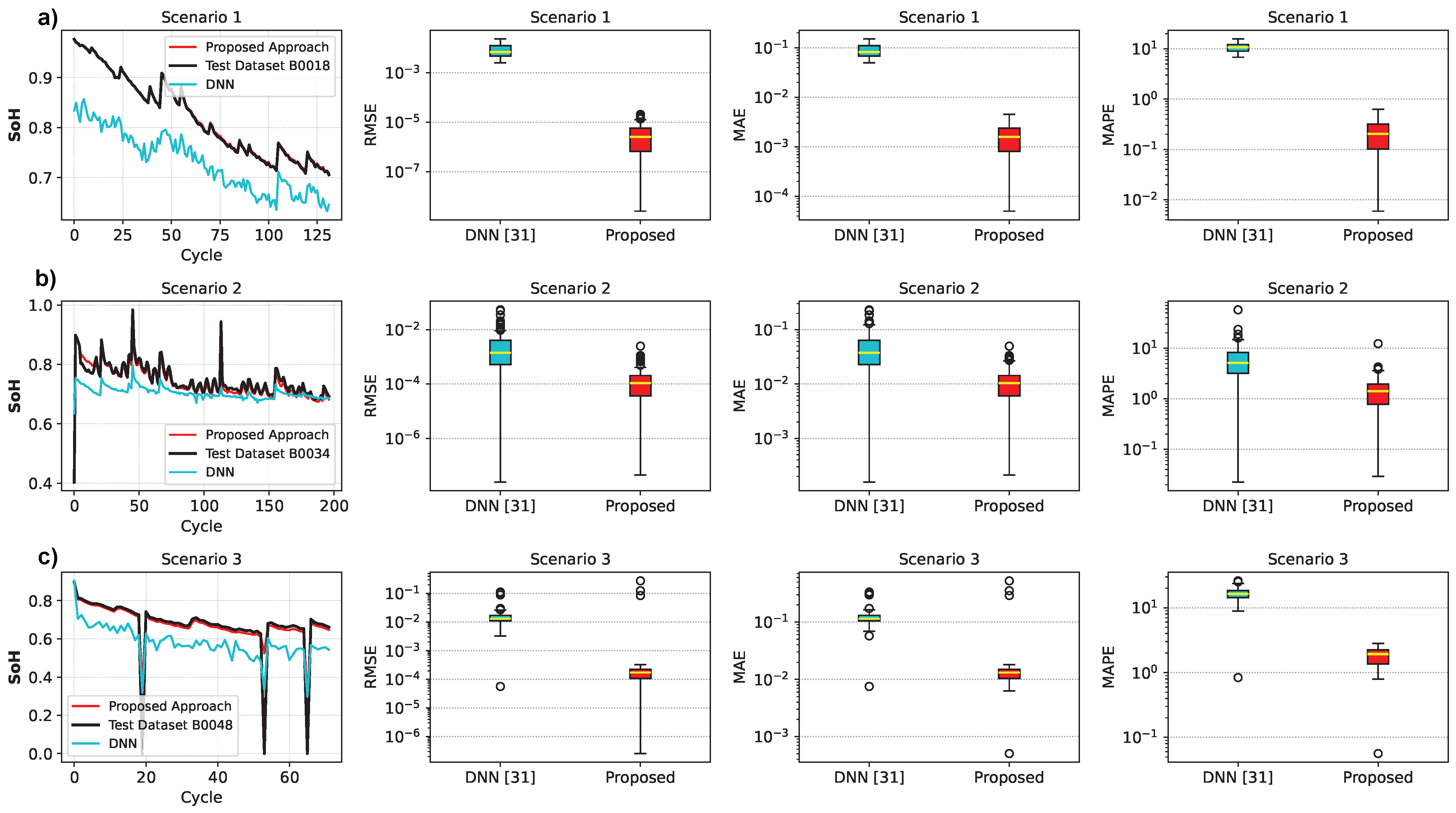
3.5. Data-Driven Robustness Comparison

To evaluate the robustness [55] of our proposed aproach, we adjusted the experimental setup presented in [59] with more intense noise contamination. The original study [59] used Gaussian white noise with an SNR of 30 dB. We evaluated our model with an SNR = 10 dB. This simulated more adverse data conditions. We compared our proposed approach with the deep neural network (DNN) model for SoH estimation. The DNN model is described in [31] and summarized in Section 3.5.1. To eliminate any bias that might arise from differences in noise handling, we employed the same proposed signal reconstruction stage based on modified Tikhonov regularization for the DNN model, which was used in our proposed SoH estimation approach. Note that SoH estimations were performed across different battery aging stages, operational conditions, and charging protocols.

3.5.1. DNN

The DNN model extracts three key temporal features from the constant current–constant voltage (CC-CV) charging process: (1) the initial voltage inflection point, which characterizes the early charging behavior; (2) the CC-CV transition time, occurring when the cell reaches 4.2 V and the current decreases to 1.5 A; and (3) the time to reach peak cell temperature, which captures thermal characteristics during charging. The DNN architecture consists of two hidden layers with three neurons each, employing Rectified Linear Unit (ReLU) activation functions between layers.

As illustrated in Figure 4, our proposed approach consistently estimates the SoH throughout the battery life cycles. The temporary increment in the measured value of SoH (non-linearities) in Figure 4 corresponds to the capacity regeneration phenomenon that occurs in lithium-ion batteries [60]. Our approach demonstrates superior robustness against noise, particularly in Scenario 2, where the presence of high noise levels significantly affects the DNN model [31]. While DNN models require large datasets for effective learning, our method achieves comparable or superior performance with significantly fewer training samples in noisy conditions. In addition, in Scenario 3, which includes multiple missing values in the training data, our method maintained its resilience, further demonstrating its robustness under adverse conditions.

Compared to the DNN [31] model, our proposed approach achieves superior performance (see Figure 4) with a RMSE of ${10}^{-4}$, MAE of ${10}^{-2}$, and MAPE below of 1%. These results confirm the ability of our proposed approach to perform consistent and accurate SoH estimations across different discharge conditions and with limited training data. We further benchmarked our results against prior state-of-the-art methods, as shown in Table 1.

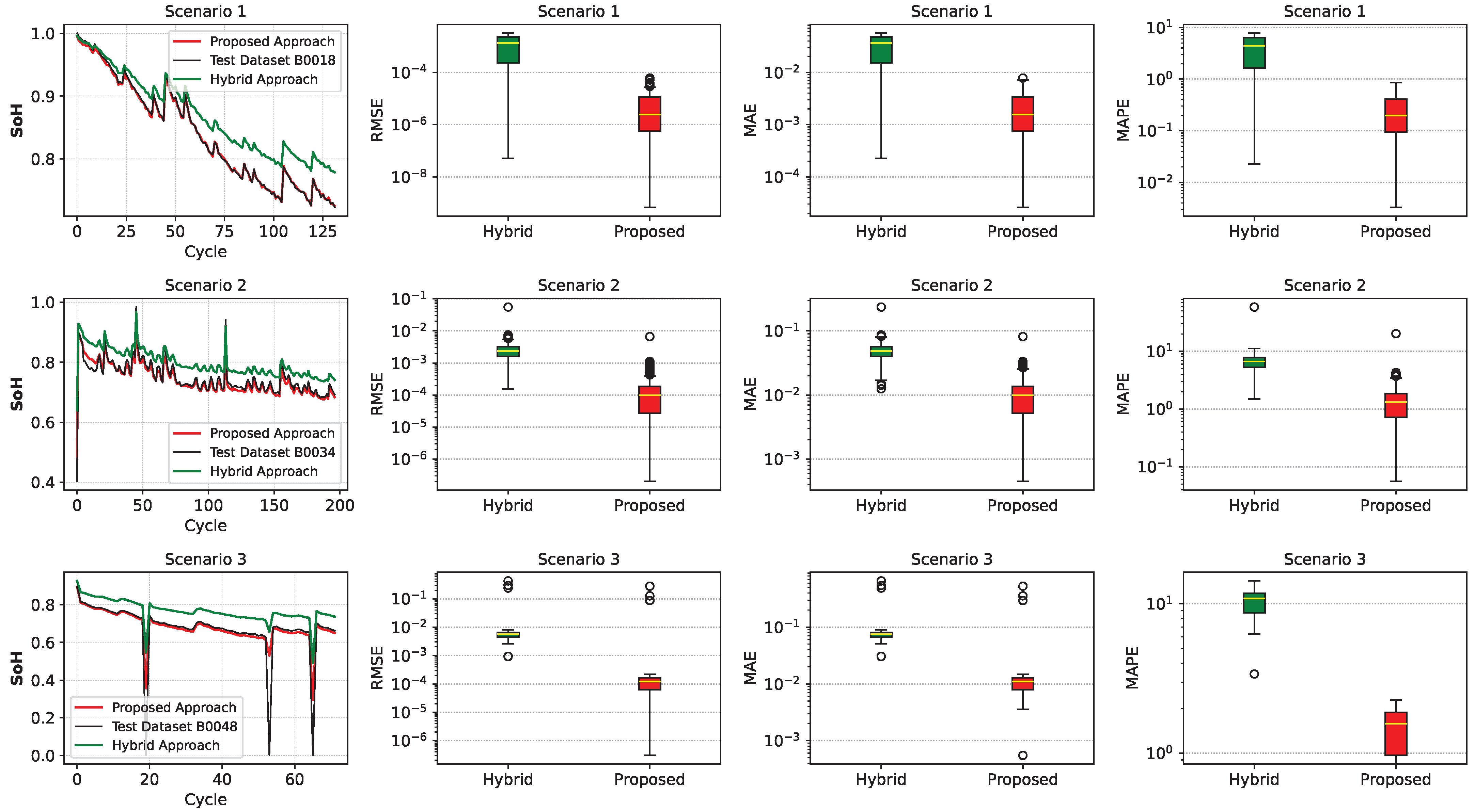
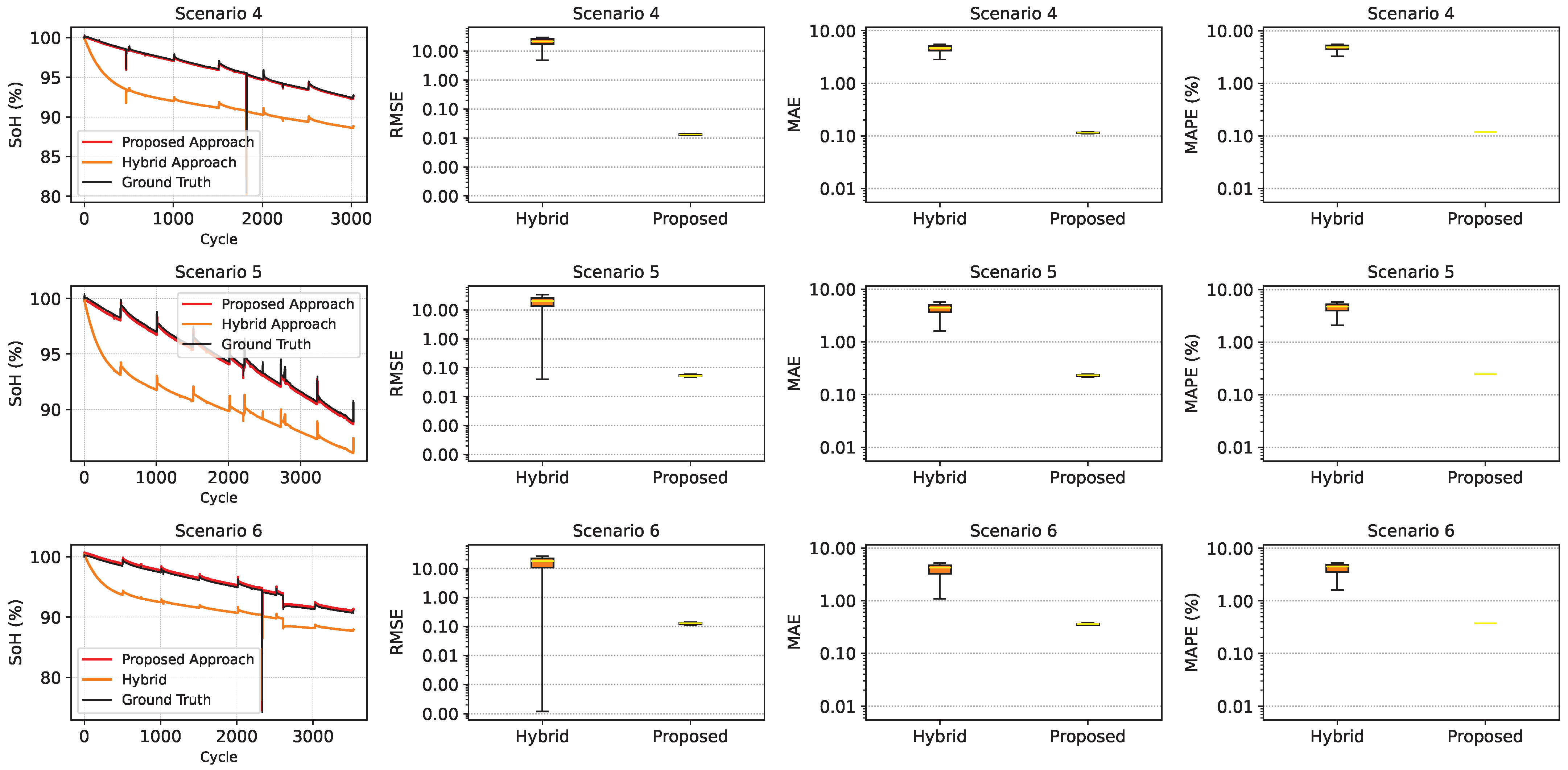
3.6. Comparison with Hybrid Model

Our proposed approach is a purely data-driven machine learning (ML) model. We compare our proposed approach with the hybrid approach in [61], which combines ML-based predictions with a physics-based model. In the test of the hybrid approach, we employed the proposed pipeline in Section 2.1 as the machine learning component. For the physics-based model, an exponential decay assumption was employed, as follows:

$${\mathrm{SoH}}_{\mathrm{phys}}\left(n\right)=C_f+\left(C_0-C_f\right)exp\left(-\beta n^{\alpha }\right)$$

(22)

where $C_0$ represents the initial capacity (normalized to 1.0), $C_f$ is the final capacity (e.g., 0.8), and $\beta ,\alpha$ are decay parameters that control how quickly the SoH degrades with cycle count. As shown in Figure 5 and Figure 6, the hybrid approach model might not perfectly capture real-world battery dynamics. This limitation underscores that our proposed data-driven method can help correct or improve these SoH estimations. To compute the following results, hybrid model fusion was weighted 30% physics and 70% ML as follows:

$${\mathrm{SoH}}_{\mathrm{hybrid}}=w·{\mathrm{SoH}}_{\mathrm{phys}}+(1-w)·{\mathrm{SoH}}_{\mathrm{ML}}$$

(23)

The hybrid approach was tested using the six scenarios presented in Section 2.2.

Table 7. Comparison of proposed state-of-health (SoH) estimator with a deep neural network (DNN) using three handcrafted charging features, a Huber-regression model trained on ten direct statistics, and a hybrid estimator (physics-aided). Performance is evaluated under six aging scenarios, with results reported as root mean square error (RMS), mean absolute error (MAE), and mean absolute percentage error (MAPE). Lower values indicate higher accuracy. Aggregated results are labeled “Average”. The best results are in bold.

Scenario	Method	RMSE	MAE	MAPE (%)
1	Proposed	0.0029	0.0022	0.2546
	DNN	0.018239	0.015416	1.9341
	Direct Features	0.0042	0.0034	0.4231
	Hybrid	2.277851	1.922806	2.5100
2	Proposed	0.0140	0.0110	1.4985
	DNN	0.103690	0.097540	12.8129
	Direct Features	0.0274	0.0238	3.2878
	Hybrid	2.845887	1.890512	2.6018
3	Proposed	0.0835	0.0261	1.4191
	DNN	0.178465	0.174136	23.8429
	Direct Features	0.0883	0.0793	10.6426
	Hybrid	10.205681	3.207709	1.7226
4	Proposed	0.0640	0.0567	0.06
	DNN	9.3996	9.3972	9.78
	Direct Features	4.5677	0.5558	0.58
	Hybrid	4.5398	4.4670	4.65
5	Proposed	0.0830	0.0757	0.08
	DNN	0.4271	0.3912	0.41
	Direct Features	4.6395	0.5065	0.53
	Hybrid	4.2480	4.1490	4.37
6	Proposed	0.2696	0.2676	0.28
	DNN	22.5040	22.4926	23.58
	Direct Features	5.5194	2.2520	2.36
	Hybrid	4.2111	4.1170	4.30
Average	Proposed	0.0862	0.0732	0.5987
	DNN	5.4385	5.4280	12.0616
	Direct Features	2.4744	0.5701	2.96725
	Hybrid	4.72140	3.2923	3.3591

compares the accuracy of the proposed SoH estimation pipeline with three alternatives over six representative aging scenarios. These results confirm that our proposed pipeline estimates SoH, even under severe noise, missing data, and variable discharge protocols, where the alternative methods lose accuracy.

As is shown in

Table 8. Comparative analysis of State of Health (SoH) estimation performance across six scenarios, demonstrating the effect of discharge C-rates, ambient temperatures, and charging protocols on RMSE, MAE, and MAPE metrics.

Scenario	Charge C-Rate	Discharge C-Rate	Ambient Temperature (°C)	RMS	MAE	MAPE (%)
1	∼0.75C (CC-CV)	1C	4 to 40	0.002021	0.001711	0.2182
2	∼0.75C (CC-CV)	1C	24	0.013571	0.011308	1.5269
3	∼0.75C (CC-CV)	2C	4	0.083121	0.028124	1.8028
4	∼0.75C (CC-CV)	1C	25	0.1148	0.1147	0.12
5	0.5C (CC)	0.5C (CC)	15	0.2309	0.2308	0.24
6	0.5C (CC)	2C (CC)	25	0.3568	0.3566	0.37

, SoH estimation of lithium-ion batteries is influenced by operational parameters such as discharge C-rates, temperature, and charging protocols. In this case, higher discharge C-rates tend to larger estimation errors. However, our proposed approach maintains competitive accuracy. Low temperatures like 4 °C lead to higher errors compared to moderate temperatures such as 24 °C. The CC-CV charging protocol performs better than CC for SoH estimation.

4. Conclusions

This study demonstrates that the robustness of state-of-health estimation for lithium-ion batteries is significantly influenced by the choice of machine learning architecture, loss function, feature selection, and signal reconstruction technique. The performance of our proposed approach remained stable under low-temperature (4 °C) operation, high discharge rates (2C), severe Gaussian noise (10 dB SNR), and missing data, where DNN and hybrid models lost accuracy. This work also demonstrated that well-engineered features, obtained using domain knowledge, capture relevant information more effectively than a larger quantity of statistics. In this case, our proposed approach, which relies on only five engineered features, outperformed a comparable model that used ten statistical features.

Our proposed closed-form signal reconstruction approach based on modified Tikhonov regularization achieves superior reconstruction quality across various noise levels, compared to the iterative LASSO, moving average filter, and Kalman filter. Our proposed data-driven SoH estimation approach demonstrated high accuracy under noisy conditions, with a low computational cost.

Future research will aim to extend our proposed SoH estimation approach by incorporating additional relevant physical parameters, developing adaptive methods for selecting the regularization parameter ($\delta$), and performing experiments using non-Gaussian noise and extreme operating conditions. Our current results strongly highlight the potential of data-driven methods for achieving accurate and robust SoH estimation within battery management systems (BMS), which are critical for the safe and efficient operation of electric vehicles (EV). Hence, future work will focus on validating our proposed approach under more diverse and variable battery aging conditions, using real-world EVs datasets.

References

1. Greim, P.; Solomon, A.; Breyer, C. Assessment of lithium criticality in the global energy transition and addressing policy gaps in transportation. Nat. Commun. 2020, 11, 4570. [Google Scholar] [CrossRef]
2. Lagrange, A.; de Simón-Martín, M.; González-Martínez, A.; Bracco, S.; Rosales-Asensio, E. Sustainable microgrids with energy storage as a means to increase power resilience in critical facilities: An application to a hospital. Int. J. Electr. Power Energy Syst. 2020, 119, 105865. [Google Scholar] [CrossRef]
3. Department of Energy. DOE Global Energy Storage Database, 2023. Available online: https://gesdb.sandia.gov/ (accessed on 8 September 2023).
4. Stroe, D.I.; Schaltz, E. Lithium-ion battery state-of-health estimation using the incremental capacity analysis technique. IEEE Trans. Ind. Appl. 2019, 56, 678–685. [Google Scholar] [CrossRef]
5. Kallel, A.Y.; Petrychenko, V.; Kanoun, O. State-of-health of Li-ion battery estimation based on the efficiency of the charge transfer extracted from impedance spectra. Appl. Sci. 2022, 12, 885. [Google Scholar] [CrossRef]
6. Oji, T.; Zhou, Y.; Ci, S.; Kang, F.; Chen, X.; Liu, X. Data-driven methods for battery soh estimation: Survey and a critical analysis. IEEE Access 2021, 9, 126903–126916. [Google Scholar] [CrossRef]
7. John, J.; Kudva, G.; Jayalakshmi, N. Secondary life of electric vehicle batteries: Degradation, state of health estimation using incremental capacity analysis, applications and challenges. IEEE Access 2024, 12, 63735–63753. [Google Scholar] [CrossRef]
8. Gharebaghi, M.; Rezaei, O.; Li, C.; Wang, Z.; Tang, Y. A Survey on Using Second-Life Batteries in Stationary Energy Storage Applications. Energies 2024, 18, 42. [Google Scholar] [CrossRef]
9. Zhang, J.; Li, K. State-of-Health Estimation for Lithium-Ion Batteries in Hybrid Electric Vehicles—A Review. Energies 2024, 17, 5753. [Google Scholar] [CrossRef]
10. Liu, K.; Wang, Y.; Lai, X. Data Science-Based Full-Lifespan Management of Lithium-Ion Battery: Manufacturing, Operation and Reutilization; Springer Nature: Berlin/Heidelberg, Germany, 2022. [Google Scholar]
11. Tian, J.; Xiong, R.; Shen, W. A review on state of health estimation for lithium ion batteries in photovoltaic systems. ETransportation 2019, 2, 100028. [Google Scholar] [CrossRef]
12. Wilhelm, J.; Seidlmayer, S.; Keil, P.; Schuster, J.; Kriele, A.; Gilles, R.; Jossen, A. Cycling capacity recovery effect: A coulombic efficiency and post-mortem study. J. Power Sources 2017, 365, 327–338. [Google Scholar] [CrossRef]
13. Bayoumi, E.H.; De Santis, M.; Awad, H. A Brief Overview of Modeling Estimation of State of Health for an Electric Vehicle’s Li-Ion Batteries. World Electr. Veh. J. 2025, 16, 73. [Google Scholar] [CrossRef]
14. Andersson, M.; Streb, M.; Ko, J.Y.; Klass, V.L.; Klett, M.; Ekström, H.; Johansson, M.; Lindbergh, G. Parametrization of physics-based battery models from input–output data: A review of methodology and current research. J. Power Sources 2022, 521, 230859. [Google Scholar] [CrossRef]
15. Iurilli, P.; Brivio, C.; Carrillo, R.E.; Wood, V. Physics-Based SoH Estimation for Li-Ion Cells. Batteries 2022, 8, 204. [Google Scholar] [CrossRef]
16. Sun, X.; Zhang, Y.; Zhang, Y.; Wang, L.; Wang, K. Summary of health-state estimation of lithium-ion batteries based on electrochemical impedance spectroscopy. Energies 2023, 16, 5682. [Google Scholar] [CrossRef]
17. Tran, M.K.; Mathew, M.; Janhunen, S.; Panchal, S.; Raahemifar, K.; Fraser, R.; Fowler, M. A comprehensive equivalent circuit model for lithium-ion batteries, incorporating the effects of state of health, state of charge, and temperature on model parameters. J. Energy Storage 2021, 43, 103252. [Google Scholar] [CrossRef]
18. Velasco-Arellano, H.; Castillo-Magallanes, N.; Visairo-Cruz, N.; Núñez-Gutiérrez, C.A.; Lázaro, I. Parametric Correlation Analysis between Equivalent Electric Circuit Model and Mechanistic Model Interpretation for Battery Internal Aging. World Electr. Veh. J. 2024, 15, 291. [Google Scholar] [CrossRef]
19. Lu, J.; Wu, T.; Amine, K. State-of-the-art characterization techniques for advanced lithium-ion batteries. Nat. Energy 2017, 2, 1–13. [Google Scholar] [CrossRef]
20. Ren, Z.; Du, C. A review of machine learning state-of-charge and state-of-health estimation algorithms for lithium-ion batteries. Energy Rep. 2023, 9, 2993–3021. [Google Scholar] [CrossRef]
21. Zhang, M.; Yang, D.; Du, J.; Sun, H.; Li, L.; Wang, L.; Wang, K. A review of SOH prediction of Li-ion batteries based on data-driven algorithms. Energies 2023, 16, 3167. [Google Scholar] [CrossRef]
22. Gong, J.; Xu, B.; Chen, F.; Zhou, G. Predictive Modeling for Electric Vehicle Battery State of Health: A Comprehensive Literature Review. Energies 2025, 18, 337. [Google Scholar] [CrossRef]
23. Nuroldayeva, G.; Serik, Y.; Adair, D.; Uzakbaiuly, B.; Bakenov, Z. State of health estimation methods for lithium-ion batteries. Int. J. Energy Res. 2023, 2023, 4297545. [Google Scholar] [CrossRef]
24. Alamin, K.S.S.; Daghero, F.; Pollo, G.; Pagliari, D.J.; Chen, Y.; Macii, E.; Poncino, M.; Vinco, S. Model-Driven Dataset Generation for Data-Driven Battery SOH Models. In Proceedings of the 2023 IEEE/ACM International Symposium on Low Power Electronics and Design (ISLPED), Vienna, Austria, 7–8 August 2023; pp. 1–6. [Google Scholar]
25. Bamati, S.; Chaoui, H. Developing an online data-driven state of health estimation of lithium-ion batteries under random sensor measurement unavailability. IEEE Trans. Transp. Electrif. 2022, 9, 1128–1141. [Google Scholar] [CrossRef]
26. Wang, J.; Zhang, C.; Meng, X.; Zhang, L.; Li, X.; Zhang, W. A Novel Feature Engineering-Based SOH Estimation Method for Lithium-Ion Battery with Downgraded Laboratory Data. Batteries 2024, 10, 139. [Google Scholar] [CrossRef]
27. Zhang, Z.; Zhang, R.; Liu, X.; Zhang, C.; Sun, G.; Zhou, Y.; Yang, Z.; Liu, X.; Chen, S.; Dong, X.; et al. Advanced State-of-Health Estimation for Lithium-Ion Batteries Using Multi-Feature Fusion and KAN-LSTM Hybrid Model. Batteries 2024, 10, 433. [Google Scholar] [CrossRef]
28. Lu, X.; Qiu, J.; Lei, G.; Zhu, J. Degradation mode knowledge transfer method for LFP batteries. IEEE Trans. Transp. Electrif. 2022, 9, 1142–1152. [Google Scholar] [CrossRef]
29. Lu, X.; Qiu, J.; Lei, G.; Zhu, J. State of health estimation of lithium iron phosphate batteries based on degradation knowledge transfer learning. IEEE Trans. Transp. Electrif. 2023, 9, 4692–4703. [Google Scholar] [CrossRef]
30. Alhazmi, R.M. State of health prediction in electric vehicle batteries using a deep learning model. World Electr. Veh. J. 2024, 15, 385. [Google Scholar] [CrossRef]
31. Driscoll, L.; de la Torre, S.; Gomez-Ruiz, J.A. Feature-based lithium-ion battery state of health estimation with artificial neural networks. J. Energy Storage 2022, 50, 104584. [Google Scholar] [CrossRef]
32. Khumprom, P.; Yodo, N. A data-driven predictive prognostic model for lithium-ion batteries based on a deep learning algorithm. Energies 2019, 12, 660. [Google Scholar] [CrossRef]
33. Cui, Z.; Wang, C.; Gao, X.; Tian, S. State of health estimation for lithium-ion battery based on the coupling-loop nonlinear autoregressive with exogenous inputs neural network. Electrochim. Acta 2021, 393, 139047. [Google Scholar] [CrossRef]
34. Fan, Y.; Xiao, F.; Li, C.; Yang, G.; Tang, X. A novel deep learning framework for state of health estimation of lithium-ion battery. J. Energy Storage 2020, 32, 101741. [Google Scholar] [CrossRef]
35. Zhou, D.; Li, Z.; Zhu, J.; Zhang, H.; Hou, L. State of health monitoring and remaining useful life prediction of lithium-ion batteries based on temporal convolutional network. IEEE Access 2020, 8, 53307–53320. [Google Scholar] [CrossRef]
36. Acurio, B.A.A.; Barragán, D.E.C.; Amezquita, J.C.L.; Rider, M.J.; Da Silva, L.C.P. Design and Implementation of a Machine Learning State Estimation Model for Unobservable Microgrids. IEEE Access 2022, 10, 123387–123398. [Google Scholar] [CrossRef]
37. Rufino Júnior, C.A.; Sanseverino, E.R.; Gallo, P.; Amaral, M.M.; Koch, D.; Kotak, Y.; Diel, S.; Walter, G.; Schweiger, H.G.; Zanin, H. Unraveling the degradation mechanisms of lithium-ion batteries. Energies 2024, 17, 3372. [Google Scholar] [CrossRef]
38. Wei, Y.; Yao, Y.; Pang, K.; Xu, C.; Han, X.; Lu, L.; Li, Y.; Qin, Y.; Zheng, Y.; Wang, H.; et al. A comprehensive study of degradation characteristics and mechanisms of commercial Li (NiMnCo) O2 EV batteries under vehicle-to-grid (V2G) services. Batteries 2022, 8, 188. [Google Scholar] [CrossRef]
39. Yagci, M.C.; Feldmann, T.; Bollin, E.; Schmidt, M.; Bessler, W.G. Aging characteristics of stationary lithium-ion battery systems with serial and parallel cell configurations. Energies 2022, 15, 3922. [Google Scholar] [CrossRef]
40. Edge, J.S.; O’Kane, S.; Prosser, R.; Kirkaldy, N.D.; Patel, A.N.; Hales, A.; Ghosh, A.; Ai, W.; Chen, J.; Yang, J.; et al. Lithium ion battery degradation: What you need to know. Phys. Chem. Chem. Phys. 2021, 23, 8200–8221. [Google Scholar] [CrossRef]
41. Yang, X.; Wang, Z.; Xie, S. Influence of Overdischarge Depth on the Aging and Thermal Safety of LiNi0.5Co0.2Mn0.3O2/Graphite Cells. Battery Energy 2025, e70008. [Google Scholar] [CrossRef]
42. Li, S.; Ke, B. Study of battery modeling using mathematical and circuit oriented approaches. In Proceedings of the 2011 IEEE Power and Energy Society General Meeting, Detroit, MI, USA, 24–29 July 2011; pp. 1–8. [Google Scholar]
43. Birkl, C.R.; Roberts, M.R.; McTurk, E.; Bruce, P.G.; Howey, D.A. Degradation diagnostics for lithium ion cells. J. Power Sources 2017, 341, 373–386. [Google Scholar] [CrossRef]
44. Shen, W.; Wang, N.; Zhang, J.; Wang, F.; Zhang, G. Heat generation and degradation mechanism of lithium-ion batteries during high-temperature aging. ACS Omega 2022, 7, 44733–44742. [Google Scholar] [CrossRef]
45. Huang, R.; Xu, Y.; Wu, Q.; Chen, J.; Chen, F.; Yu, X. Simulation study on heat generation characteristics of lithium-ion battery aging process. Electronics 2023, 12, 1444. [Google Scholar] [CrossRef]
46. Wang, Q.; Ma, Y.; Zhao, K.; Tian, Y. A comprehensive survey of loss functions in machine learning. Ann. Data Sci. 2020, 9, 187–212. [Google Scholar] [CrossRef]
47. Mangasarian, O.L.; Musicant, D.R. Robust linear and support vector regression. IEEE Trans. Pattern Anal. Mach. Intell. 2000, 22, 950–955. [Google Scholar] [CrossRef]
48. Huber, P.J. Robust estimation of a location parameter. In Breakthroughs in Statistics: Methodology and Distribution; Springer: Berlin/Heidelberg, Germany, 1992; pp. 492–518. [Google Scholar]
49. Saha, B.; Goebel, K. Battery data set. In NASA AMES Prognostics Data Repository; NASA Ames Research Center: Moffett Field, CA, USA, 2007. Available online: https://www.nasa.gov/intelligent-systems-division/discovery-and-systems-health/pcoe/pcoe-data-set-repository/ (accessed on 1 January 2023).
50. Preger, Y.; Barkholtz, H.M.; Fresquez, A.; Campbell, D.L.; Juba, B.W.; Romàn-Kustas, J.; Ferreira, S.R.; Chalamala, B. Degradation of commercial lithium-ion cells as a function of chemistry and cycling conditions. J. Electrochem. Soc. 2020, 167, 120532. [Google Scholar] [CrossRef]
51. Ma, S.; Jiang, M.; Tao, P.; Song, C.; Wu, J.; Wang, J.; Deng, T.; Shang, W. Temperature effect and thermal impact in lithium-ion batteries: A review. Prog. Nat. Sci. Mater. Int. 2018, 28, 653–666. [Google Scholar] [CrossRef]
52. Battery Archive. Battery Archive, 2025. Available online: https://www.batteryarchive.org/ (accessed on 6 March 2025).
53. Lipu, M.S.H.; Mamun, A.A.; Ansari, S.; Miah, M.S.; Hasan, K.; Meraj, S.T.; Abdolrasol, M.G.; Rahman, T.; Maruf, M.H.; Sarker, M.R.; et al. Battery management, key technologies, methods, issues, and future trends of electric vehicles: A pathway toward achieving sustainable development goals. Batteries 2022, 8, 119. [Google Scholar] [CrossRef]
54. Python Software Foundation. Python Programming Language; Python Software Foundation: Wilmington, DE, USA, 1991–2024; Available online: https://www.python.org/ (accessed on 1 January 2023).
55. Lucu, M.; Martinez-Laserna, E.; Gandiaga, I.; Camblong, H. A critical review on self-adaptive Li-ion battery ageing models. J. Power Sources 2018, 401, 85–101. [Google Scholar] [CrossRef]
56. Engelberg, S. Implementing Moving Average Filters Using Recursion [Tips & Tricks]. IEEE Signal Process. Mag. 2023, 40, 78–80. [Google Scholar]
57. Kim, Y.; Bang, H. Introduction to Kalman filter and its applications. In Introduction and Implementations of the Kalman Filter; IntechOpen: Rijeka, Croatia, 2018. [Google Scholar]
58. Jiang, N.; Zhang, J.; Jiang, W.; Ren, Y.; Lin, J.; Khoo, E.; Song, Z. Driving behavior-guided battery health monitoring for electric vehicles using extreme learning machine. Appl. Energy 2024, 364, 123122. [Google Scholar] [CrossRef]
59. Lin, M.; Zeng, X.; Wu, J. State of health estimation of lithium-ion battery based on an adaptive tunable hybrid radial basis function network. J. Power Sources 2021, 504, 230063. [Google Scholar] [CrossRef]
60. Deng, L.M.; Hsu, Y.C.; Li, H.X. An improved model for remaining useful life prediction on capacity degradation and regeneration of lithium-ion battery. In Proceedings of the Annual Conference of the PHM Society, Jeju, Republic of Korea, 2–5 October 2017; Volume 9. [Google Scholar]
61. Liang, J.; Liu, H.; Xiao, N.C. A hybrid approach based on deep neural network and double exponential model for remaining useful life prediction. Expert Syst. Appl. 2024, 249, 123563. [Google Scholar] [CrossRef]
Figure 1. Proposed state of health estimation for lithium-ion batteries based on signal reconstruction.
Energies 18 02459 g001
Figure 2. Sensitivity analysis of signal reconstruction quality across various SNRs (10–50 dB). Our proposed approach based on Tikhonov consistently outperforms widely adopted signal processing methods, including the LASSO formulation, moving average (MA) filter, and the Kalman filter, across multiple accuracy metrics. Boxplots show (a) RMSE, (b) MAE, and (c) MAPE, with the proposed approach yielding the lowest error dispersion across all metrics, highlighting its effectiveness in preserving signal quality under noise.
Energies 18 02459 g002
Figure 3. Performance comparison of state-of-health (SoH) estimation across three scenarios using direct features reported in [58] vs. our proposed feature selection approach. In each scenario, the left plot shows predicted SoH at different numbers of aging cycles. The boxplots show RMSE, MAE, and MAPE. The proposed method consistently exhibits lower prediction errors, highlighting its effectiveness over direct features.
Energies 18 02459 g003
Figure 4. (a) In Scenario 1, our proposed approach consistently estimates the SoH throughout the battery life cycle. (b) In Scenario 2, the comparison highlights the robustness of our proposed approach against noisy data, whereas the DNN approach [31] is sensitive to noise. (c) In Scenario 3, the results demonstrate the resilience of our proposed approach to some missing values.
Energies 18 02459 g004
Figure 5. Comparison of proposed SoH approach (red) versus hybrid model (green) [61] across multiple scenarios based on NASA dataset [49] and detailed in Section 2.2. Left plots show the SoH predictions for each scenario along different numbers of aging cycles (the ground truth is in black). Boxplots of the corresponding error metrics RMSE, MAE, and MAPE. Overall, our proposed purely data-driven approach captures real-world battery aging dynamics more accurately and consistently than the hybrid model.
Energies 18 02459 g005
Figure 6. Comparison of proposed SoH approach (red) versus hybrid model (orange) [61], across multiple scenarios based on SNL dataset [50] and detailed in Section 2.2. Left plots show the SoH predictions for each scenario along different numbers of aging cycles (the ground truth is in black). Boxplots of the corresponding error metrics RMSE, MAE, and MAPE. We can see our proposed pure data-driven approach can adapt to the nuances of battery aging in ways the hybrid approach could not.
Energies 18 02459 g006